Article

Community Detection of Multi-Layer Attributed Networks via Penalized Alternating Factorization

KLAS of MOE & School of Mathematics and Statistics, Northeast Normal University, Changchun 130024, China
*
Author to whom correspondence should be addressed.
Mathematics 2020, 8(2), 239; https://doi.org/10.3390/math8020239
Submission received: 1 January 2020 / Revised: 8 February 2020 / Accepted: 8 February 2020 / Published: 13 February 2020
(This article belongs to the Section Computational and Applied Mathematics)

Abstract

:
Communities are often associated with important structural characteristics of a complex network system, therefore detecting communities is considered to be a fundamental problem in network analysis. With the development of data collection technology and platform, more and more sources of network data are acquired, which makes the form of network as well as the related data more complex. To achieve integrative community detection of a multi-layer attributed network that involves multiple network layers together with their attribute data, effectively utilizing the information from the multiple networks and the attributes may greatly enhance the accuracy of community detection. To this end, in this article, we study the integrative community detection problem of a multi-layer attributed network from the perspective of matrix factorization, and propose a penalized alternative factorization (PAF) algorithm to resolve the corresponding optimization problem, followed by the convergence analysis of the PAF algorithm. Results of the numerical study, as well as an empirical analysis, demonstrate the advantages of the PAF algorithm in community discovery accuracy and compatibility with multiple types of network-related data.

1. Introduction

Network science is one of the most active research fields in recent years [1], which has been successfully applied in many fields, including the social science to study social relationships among individuals [2], biology to study interactions among genes and proteins [3], neuroscience to study the structure and function of the brain [4], and so on. Networks can represent and analyze the relational structure among interacting units of a complex system, and in many cases, the units of a network can be divided into groups with the property that there are many edges between units in the same group, but relatively few edges between units in different groups. Such groups are known as communities, which are often associated with important structural characteristics of a complex system. [5,6].
For example, in social networks, communities can correspond to groups with common interests [7,8]. In World Wide Web networks, communities can correspond to webpages with related topics [9]; in brain networks, they can correspond to specialized functional components [10]; and in protein–protein interaction networks, they can correspond to groups of proteins that contribute to the same cellular function [11]. Communities are often useful for understanding the essential functionality and organizational principles of networks. Therefore, community detection is considered a fundamental problem in understanding and analyzing networks [6].
Community detection has been widely studied in many application fields since the 1980s. Various models and algorithms have been developed in different fields, such as machine learning, network science, social science, and statistical physics. Community detection is a computationally challenging problem because the number of possible partitions of nodes into nonoverlapping groups is non-polynomial in the size of a network, especially in large networks. To deal with this challenging problem, a large number of algorithmic approaches have been proposed [12,13,14,15,16], including various greedy algorithms, such as hierarchical clustering [17], graph partitioning [18], and the methods based on optimizing a global criterion over all possible partitions, such as normalized cuts [19] and modularity [20]. Other algorithmic approaches include spectral methods [21,22,23,24], semi-definite programming [25,26], low-rank approximation [27], and non-negative matrix factorization [28].
Recently the quantities and types of network-related data are rising very fast, as data collection technologies or platforms rapidly evolve. Consequently, a large number of studies on community detection for various types of network-related data have been conducted, which will be introduced as follows according to the type of networks they are targeting.
First, for a single network, a number of approaches to community detection have been proposed based on probabilistic models for networks with communities, such as the stochastic block model [29], the degree-corrected stochastic block model [30], and the latent factor model [31]. Other approaches by optimizing a criterion measuring the strength of community structure in some sense also have appeared, often through non-negative matrix factorization [28] and spectral approximations, such as normalized cuts [19], modularity [20,32], and many variants of spectral clustering [33,34].
For attributed network, i.e., a network together with its attribute data, several generative models for jointly modeling the edges and the attributes have been proposed, including the network random effects model [35], the embedding feature model [36], the latent variable model [37], the discriminative approach [38], the latent multi-group membership graph model [39], the social circles model for ego networks [40], the communities from edge structure and node attributes model [41], the Bayesian graph clustering model [42], the topical communities and personal interest model [43], the modified stochastic block model [44], and a criterion-based method [45].
Multi-layer network involves networks from interdependent but distinct sources [46,47], which can be simultaneously collected for a certain group of units [48]. Community detection of this type of network has been applied to a variety of problems [49,50], including clustering of temporal networks through a dynamic stochastic block model [51], modeling and analysis of air transportation routes [52], studying individuals with multiple sociometric relations [53,54], and analyzing relationships between social interactions and economic exchange [55].
In addition, in many real network data analysis, there will be a more complex or general type of network, named multi-layer attributed network, which involves multiple network layers together with their attribute data. If the multiple networks share a common community structure and the distribution of unit attributes is also correlated with this community structure, then an integrative community detection approach that can integrate information from the multiple networks as well as the attributes may make better use of all these network-related data, therefore increase the accuracy of community detection as much as possible. Unfortunately, the research on multi-layer attributed network is still in its infancy, which leads us to further explore the problem description and corresponding solution of its community detection.
To this end, in this article, we employ the framework of integrative matrix factorization to formulate and achieve community detection of a multi-layer attributed network, which can be compatible with all the special cases of a multi-layer attributed network: the single network, attributed network, and the multi-layer network. In pursuit of community discovery accuracy and compatibility with multiple types of network-related data, we propose to use the penalized alternative factorization, named the PAF algorithm, to resolve the corresponding optimization problem.
The rest of this article is organized as follows. We elaborate the community detection problem of multi-layer attributed network in Section 2, and present the PAF algorithm to learn communities in Section 3, followed by the theoretical analysis of PAF in Section 4. The numerical performance of PAF is demonstrated in Section 5, and an empirical analysis is demonstrated in Section 6. Finally, we conclude this article in Section 7 and relegate the technical proofs to Appendix A and Appendix B.

2. Problem Formulation

In this section, we will describe in detail the problems of community detection based on matrix factorization from the single network to the multi-layer attributed networks.

2.1. Single Network

Let G = ( N , E ) denote a single network, where N = { 1 , ... , n } is the node set that represents the units of the modeled system, and E N × N is the edge set containing all pairs of nodes ( u , v ) such that nodes u and v share a social, physical, or functional relationship, where N × N denotes the Cartesian product of N and N. A network G can be characterized by an n × n adjacency matrix A = ( A i j ) with each A i j { 0 , 1 } , where A i j = 1 means that there exists an edge from nodes i to j in network G; otherwise, is not. The purpose of community detection is to identify a partition of N with community structure via the observed adjacency matrix A. Due to numerous definitions of communities, there are numerous approaches to implementing community detection. In view of the simplicity and effectiveness of a matrix factorization approach, in this article we consider the problem of community detection based on the framework of matrix factorization.
In the framework of matrix factorization, the problem of community detection, given a predetermined number of communities k * , can be formulated as the following optimization problem,
min C R n × k * S R k * × k * A C S C T F 2 ,
where C is the unknown n × k * matrix used to find k * communities, S is the unknown k * × k * weight matrix, and · F denotes the Frobenius norm. This optimization problem is the same as that studied in [28], except that in our optimization problem the non-negative constraints on matrix elements of C and S are removed to improve computational efficiency. The matrix C can be viewed as the community label matrix of A. By treating each row of C as a point in R k * , we divide these points into k * clusters via k-means or any other clustering algorithm. Then, we assign the network node i N to community k { 1 , ... , k * } if and only if row i of matrix C is assigned to cluster k.
From a statistical point of view, we find that the above optimization problem (1) is closely related to the well-known stochastic block model (SBM) [29]. Specifically, under the k * -community SBM with the n × k * ground truth label matrix C ( 0 ) and the k * × k * connectivity probability matrix S ( 0 ) , once the diagonal elements of the adjacency matrix A are also considered as random terms, not fixed to be zero, then the conditional expectation of A given C ( 0 ) is
E ( A | C ( 0 ) ) = C ( 0 ) S ( 0 ) C ( 0 ) T .
Similar to the least-squares method, the ground truth labels C ( 0 ) can be predicted by minimizing the sum of squares of the observations A i j ’s and their conditional expectation E ( A i j | C ) ’s:
min C { 0 , 1 } n × k * S [ 0 , 1 ] k * × k * A E ( A | C ) F 2 = min C { 0 , 1 } n × k * S [ 0 , 1 ] k * × k * A C S C T F 2 ,
subject to j = 1 k * C i j = 1 for each i { 1 , ... , n } . This minimization problem is very hard to achieve, as the range of C, { C { 0 , 1 } n × k * : j = 1 k * C i j = 1 } , includes k * n values. Consequently, to make the corresponding calculation feasible, (3) may be relaxed into (1), if the accuracy of community recovery can be guaranteed. Note that in (1), the ranges of C and S are relaxed into the Euclidean spaces R n × k * and R k * × k * , respectively, whereas in other methods, such as the non-negative matrix factorization methods [28], the ranges can be relaxed into R + n × k * and R + k * × k * . Here, we remove the non-negative constraints to improve computational efficiency and compatibility of the proposed method, which will be explained in the following section.

2.2. Multi-Layer Attributed Network

Once the structural information from multiple sources and the attribution information of the network nodes can be collected together, we will consider the so-called multi-layer attributed network, which is written as G A t t M u l = ( N , E ( 1 ) , ... , E ( m * ) , X ) and characterized by m * n × n adjacent matrices { A ( 1 ) , ... , A ( m * ) } as well as an n × p attribution matrix X. This is a unified framework, which can include the single network, multi-layer network, and attributed network. To achieve community detection of G A t t M u l , we study the following integrative matrix factorization problem,
min C R n × k * S ( 1 ) , ... , S ( M ) R k * × k * V R p × k * m = 1 m * ω m A ( m ) C S ( m ) C T F 2 + ω 0 X C V T F 2 ,
where { ω m } m = 0 m * with m = 0 m * ω m = 1 are the weight parameters specified beforehand and V is a p × k * matrix as the right part of the matrix factorization of X. Similarly, to solve (4), we consider the following approximate minimization problem,
min C R n × k * S ( 1 ) , ... , S ( m * ) R k * × k * V R p × k * m = 1 m * ω m A ( m ) C ( 1 ) S ( m ) C ( 2 ) F 2 + ω 0 2 t = 1 2 X C ( t ) V T F 2 + λ C ( 1 ) C ( 2 ) F 2 + ν { C ( 1 ) F 2 + C ( 2 ) F 2 + V F 2 + m = 1 m * S ( m ) F 2 } .
Note that throughout this section, the weights { ω m } m = 0 m * need to be given beforehand by the users according to background knowledge. To determine these weights, one user may have to take into account the importance and scale of data from each source. If no additional information is available, for simplicity, the weights can be equally distributed.

3. Learning Algorithm

We present a penalized alternating factorization (PAF) scheme to minimize (5). In particular, the objective function is minimized step by step by fixing any m * + 2 matrices in { C ( 1 ) , C ( 2 ) , S ( 1 ) , ... , S ( m * ) , V } and then optimizing the objective function with respect to the remaining one. The algorithm is described in details as follows.
Algorithm 1 Penalized Alternating Factorization (PAF) Algorithm.
Input: 
m * n × n adjacent matrices { A ( 1 ) , ... , A ( m * ) } , an n × p attribution matrix X, the number of communities k * .
Output: 
a length-n community label vector L = ( L 1 , ... , L n ) .
1:
Initialization:
2:
(a) t = 0 ; C ( 1 , 1 ) and C ( 2 , 1 ) are both n × k * zero matrix.
3:
(b) apply SCP, the spectral clustering with perturbations [33], to A * = m = 1 m * ω m A ( m ) and find k * initial communities, transform the resulting length-n community label vector into the n × k * community label matrix, then make C ( 1 , 0 ) and C ( 2 , 0 ) equal to this initial community label matrix, where C ( 1 , 0 ) , C ( 2 , 0 ) R n × k * are initial chooses of C ( 1 ) , C ( 2 ) respectively.
4:
(c) let
V ( 0 ) = X T C ( 1 , 0 ) + C ( 2 , 0 ) C ( 1 , 0 ) T C ( 1 , 0 ) + C ( 2 , 0 ) T C ( 2 , 0 ) 1 , S ( m , 0 ) = [ C ( 1 , 0 ) T C ( 1 , 0 ) ] 1 C ( 1 , 0 ) T A ( m ) C ( 2 , 0 ) [ C ( 2 , 0 ) T C ( 2 , 0 ) ] 1 .
5:
while C ( 1 , t 1 ) , C ( 2 , t 1 ) , C ( 1 , t ) , C ( 2 , t ) are not equal do
6:
(a) given C ( 2 , t ) , { S ( m , t ) } m = 1 m * , V ( t ) , update C ( 1 , t + 1 ) by
m = 1 m * ω m A ( m ) C ( 2 , t ) S ( m , t ) T + ω 0 2 X V ( t ) + λ m = 1 m * ω m C ( 2 , t ) S ( m , t ) T T C ( 2 , t ) S ( m , t ) T + ω 0 2 V ( t ) T V ( t ) + ( λ + ν ) I k * 1 ;
7:
(b) given C ( 1 , t + 1 ) , { S ( m , t ) } m = 1 m * , V ( t ) , update C ( 2 , t + 1 ) by
m = 1 m * ω m A ( m ) T C ( 1 , t + 1 ) S ( m , t ) + ω 0 2 X V ( t ) + λ m = 1 m * ω m C ( 1 , t + 1 ) S ( m , t ) T C ( 1 , t + 1 ) S ( m , t ) + ω 0 2 V ( t ) T V ( t ) + ( λ + ν ) I k * 1 ;
8:
(c) given C ( 1 , t + 1 ) , C ( 2 , t + 1 ) , V ( t ) , update S ( m , k + 1 ) for each m { 1 , ... , m * } as follows,
vec ( S ( m , k + 1 ) ) = ω m B ( 2 , k + 1 ) T B ( 1 , k + 1 ) + ( α + ν ) I k * 1 vec ( U ( m , k + 1 ) ) ,
where B ( 1 , k + 1 ) = C ( 1 , t + 1 ) T C ( 1 , t + 1 ) , B ( 2 , k + 1 ) = C ( 2 , t + 1 ) T C ( 2 , t + 1 ) , U ( m , k + 1 ) = ω m C ( 1 , t + 1 ) T A ( m ) C ( 2 , t + 1 ) α S ( m , t ) , and v e c ( · ) denotes the vectorization of a matrix by stacking its columns and ⊗ is the Kronecker product of two matrices;
9:
(d) given C ( 1 , t + 1 ) , C ( 2 , t + 1 ) , { S ( m , k + 1 ) } m = 1 m * , update V ( t + 1 ) by
X T C ( 1 , t + 1 ) + C ( 2 , t + 1 ) + 2 β / ω 0 V ( t ) C ( 1 , t + 1 ) T C ( 1 , t + 1 ) + C ( 2 , t + 1 ) T C ( 2 , t + 1 ) + 2 ( β + ν ) / ω 0 1 ;
10:
(e) t = t + 1 .
11:
end while
12:
return the community label vector L by applying k-means to cluster the rows of C ( 1 , t ) .
Here, α , β , and ν are set to be three small positive numbers, used to ensure convergence of the algorithm. Note that in the update step of the above algorithm, all the update formulas have explicit expressions. Specifically, given C ( 2 , t ) , { S ( m , t ) } m = 1 m * , V ( t ) , we update C ( 1 , t + 1 ) by
C ( 1 , t + 1 ) = arg min C ( 1 ) R n × k * { m = 1 m * ω m A ( m ) C ( 1 ) S ( m , t ) C ( 2 , t ) F 2 + ω 0 2 X C ( 1 ) V ( t ) T F 2 + λ C ( 1 ) C ( 2 , t ) F 2 + ν C ( 1 ) F 2 } ,
which has the explicit expression in in (6)
m = 1 m * ω m A ( m ) C ( 2 , t ) S ( m , t ) T + ω 0 2 X V ( t ) + λ m = 1 m * ω m C ( 2 , t ) S ( m , t ) T T C ( 2 , t ) S ( m , t ) T + ω 0 2 V ( t ) T V ( t ) + ( λ + ν ) I k * 1 .
Similarly, we update C ( 1 , t + 1 ) in (7). Then, in (8), given C ( 1 , t + 1 ) , C ( 2 , t + 1 ) , V ( t ) , we update S ( m , t + 1 ) by
S ( m , t + 1 ) = arg min S ( m ) R k * × k * ω m A ( m ) C ( 1 , t + 1 ) S ( m ) C ( 2 , t + 1 ) F 2 + α S ( m ) S ( m , t ) F 2 + ν S ( m ) F 2 .
Finally, given C ( 1 , t + 1 ) , C ( 2 , t + 1 ) , { S ( m , t + 1 ) } m = 1 m * , we update V ( t + 1 ) by
V ( t + 1 ) = arg min V R p × k * ω 0 2 l = 1 2 X C ( l , t + 1 ) V T F 2 + β V V ( t ) F 2 + ν V F 2 ,
which has the explicit expression in (9)
X T C ( 1 , t + 1 ) + C ( 2 , t + 1 ) + 2 β / ω 0 V ( t ) C ( 1 , t + 1 ) T C ( 1 , t + 1 ) + C ( 2 , t + 1 ) T C ( 2 , t + 1 ) + 2 ( β + ν ) / ω 0 1 .

4. Theoretical Analysis

Next, we consider the convergence theory of the PAF algorithm. We will present that the iteration sequence { Θ ( t ) = ( C ( 1 , t ) , C ( 2 , t ) , { S ( m , t ) } m = 1 m * , V t ) } t = 1 generated by the PAF algorithm converges to a critical point of (5).
Proposition 1.
There exist a constant δ > 0 such that for each t { 1 , 2 , ... } , Θ ( t ) F δ .
Proof. 
Please see Appendix A.1.□
Proposition 2.
For each t { 1 , 2 , ... } ,
ρ 1 Θ ( t + 1 ) Θ ( t ) F 2 [ H ( Θ ( t ) ) H ( Θ ( t + 1 ) ) ] ,
where ρ 1 = min { 2 ( λ + ν ) 2 , α , β } .
Proof. 
Please see Appendix A.2.□
Proposition 3.
For each t { 1 , 2 , ... } ,
κ ( t + 1 ) H ( Θ ( t + 1 ) ) , κ ( t + 1 ) F ρ 2 Θ ( t + 1 ) Θ ( t ) F ,
where ρ 2 = max { 4 δ ( 2 δ 3 + τ ) + 2 α , 2 ( δ 4 + τ δ M + λ ) , 2 ( 2 δ 2 + X F + β ) } .
Proof. 
Please see Appendix A.3.□
Theorem 1.
{ Θ ( t ) } converges to a critical point of H ( Θ ) .
Proof. 
Please see Appendix A.4.□

5. Numerical Study

We now present the results of some numerical study to demonstrate the performance of the PAF algorithm, and the comparison with some existing methods, abbreviated as SCP, ANMF, and NMF, respectively. SCP is the spectral clustering with perturbations [33]. ANMF and NMF are the non-negative matrix factorization methods proposed in [28] for directed and undirected networks respectively. All the network data are generated from SBM or multi-layer SBM, and the attribution data are generated from multivariate normal distributions, where the distribution parameters will be specified in each following setting. We will use the normalized mutual information (NMI) to measure the consistency between the predicted labels and the true community labels.
First, we consider the following two simulation settings for single networks and attributed networks:
I
The n × n adjacency matrix A is generated from the undirected SBM with the parameters
P = 0 . 20 0 . 12 0 . 12 0 . 20 , π = 0 . 50 0 . 50 .
Each row of the n × 2 attribution matrix is independently generated from the multivariate normal distribution N 2 ( μ k , σ 2 I 2 ) , where the kth element of μ k is 1 and the remaining element is 0, and σ 2 = 0 . 15 .
II
The same as Setting I, except that the undirected SBM is replaced by directed SBM.
The simulation results for Settings I and II are summarized in Figure 1, where SCP ( A ) , NMF ( A ) , ANMF ( A ) , and PAF ( A ) denote applying SCP, NMF, ANMF, and PAF to A, respectively, k-means ( X ) denotes applying k-means to X and PAF ( A , X ) denotes applying PAF to ( A , X ) . The results of SCP ( A ) , NMF ( A ) , ANMF ( A ) , and PAF ( A ) in Figure 1 suggest that (1) PAF is a very good alternative to NMF and ANMF in terms of accuracy of community detection, and (2) NMF, ANMF, and PAF outperform SCP in situation where directed networks are studied.
On the other hand, the comparison between PAF ( A , X ) and the other methods in Figure 1 suggests that applying k-means to the attribution data alone fails to achieve community detection; however, once the attribution data and the network data are combined, much better results can be obtained than using the network and attribution data separately.
Next, we consider the following two simulation settings for multi-layer networks and multi-layer attributed networks:
III
The m * = 3 n × n adjacent matrices { A ( 1 ) , A ( 2 ) , A ( 3 ) } are generated independently from the undirected multi-layer SBM with common community labels, where the parameters are set as follows,
P 1 = 0 . 2 0 . 2 0 . 13 0 . 2 0 . 2 0 . 13 0 . 13 0 . 13 0 . 2 , P 2 = 0 . 2 0 . 13 0 . 13 0 . 13 0 . 2 0 . 2 0 . 13 0 . 2 0 . 2 ,
P 3 = 0 . 2 0 . 13 0 . 2 0 . 13 0 . 2 0 . 13 0 . 2 0 . 13 0 . 2 , π = 0 . 3 3 ˙ 0 . 3 3 ˙ 0 . 3 3 ˙ .
Each row of the n × 3 attribution matrix is independently generated from the multivariate normal distribution N 3 ( μ k , σ 2 I 3 ) , where the kth element of μ k is 1 and the remaining elements are 0, and σ 2 = 0 . 15 .
IV
The same as Setting III, except that the undirected multi-layer SBM model is replaced by directed multi-layer SBM.
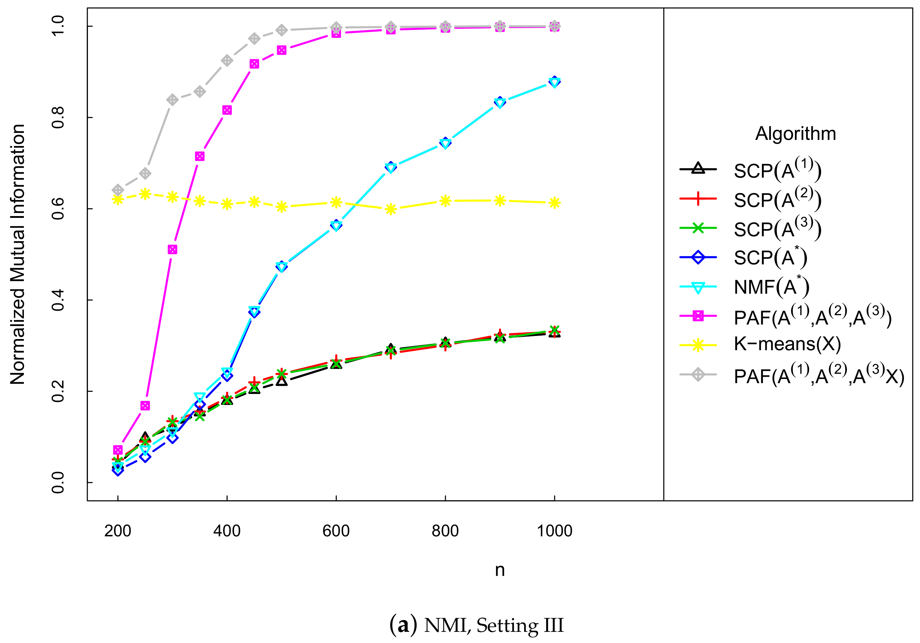
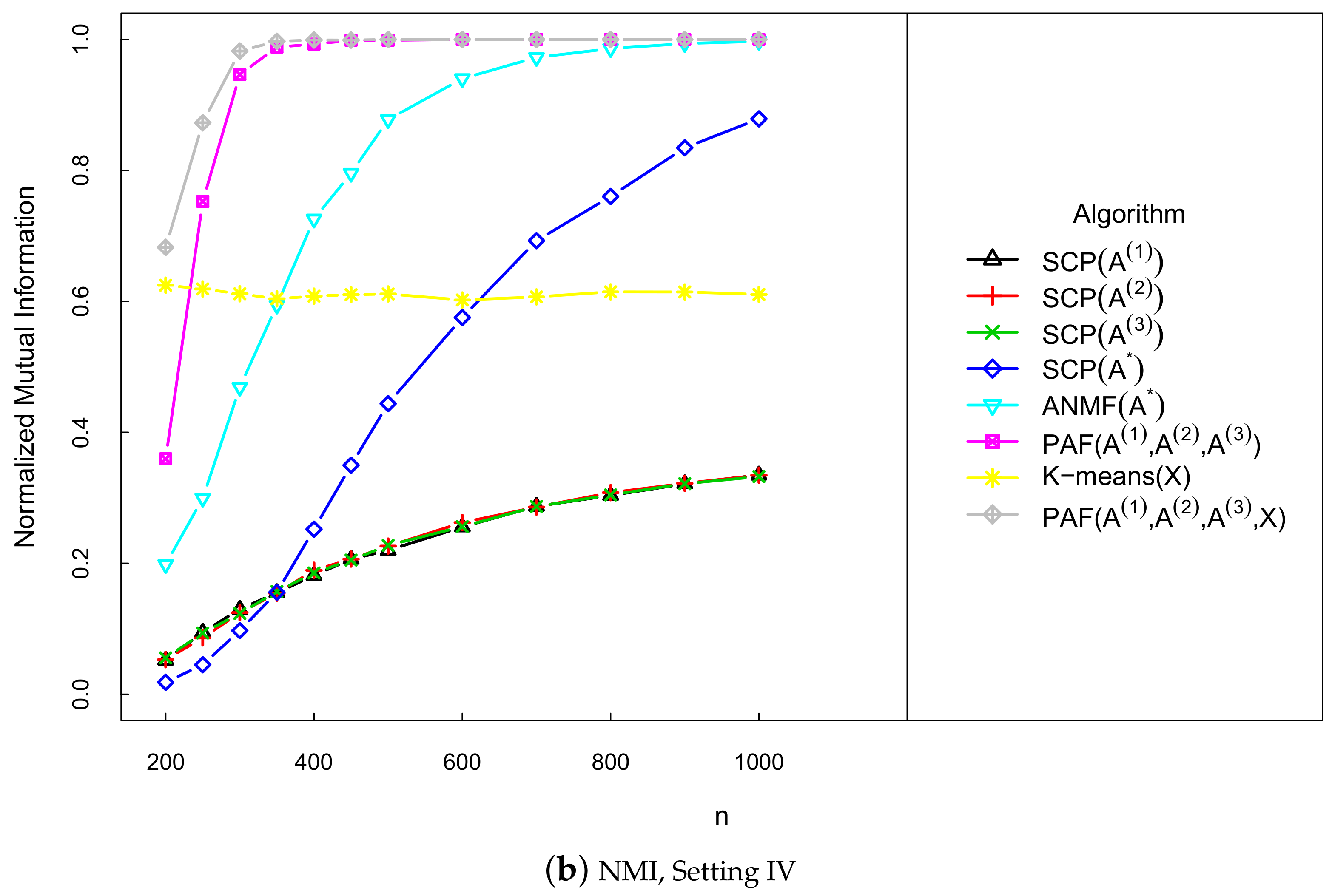
The simulation results for Settings III and IV are summarized in Figure 2, where PAF ( A ( 1 ) , A ( 2 ) , A ( 3 ) , X ) denotes applying PAF to ( A ( 1 ) , A ( 2 ) , A ( 3 ) , X ) and A * = 1 m * m = 1 m * A ( m ) . The comparison between PAF ( A ( 1 ) , A ( 2 ) , A ( 3 ) , X ) and NMF ( A * ) , ANMF ( A * ) , SCP ( A * ) , SCP ( A ( 1 ) ) , SCP ( A ( 2 ) ) , and SCP ( A ( 3 ) ) suggests that (1) integrating community information from the multiple adjacent matrices of the network layers may perform better than using each network layer separately, and (2) using the PAF algorithm to achieve integrative community detection for the multi-layer attributed network can make appropriate use of the network-related data from multiple sources.

6. Empirical Analysis

In this section, we apply the proposed PAF method to a dataset that comes from a network study of a corporate law partnership, which was carried out in a Northeastern US corporate law firm, referred to as SG&R, 1988–1991 in New England and previously studied in [45,56,57]. The dataset includes 71 attorneys of this firm and three network layers, co-work layer, advice layer, friendship layer, as well as some attributes of the attorneys, such as status (1 = partner; = associate), gender (1 = man; 2 = woman), office (1 = Boston; 2 = Hartford; 3 = Providence), years with the firm, age, practice (1 = litigation; 2 = corporate), and law school (1: Harvard, Yale; 2: UCON; 3: other). We treat the attribute “status” as the ground truth community label as in [45]. In fact, after eliminating six isolated nodes, the heatmap plots of the adjacency matrices with nodes sorted by each attribute variable indicate that the partition by “status” can present a strong assortative structure. Then, the data of the remaining six attributes together with the three network layers form a multi-layer attributed network to be studied, with m * = 3 network layers and p = 6 attribute variables, which falls right into the scope of application of the proposed method.
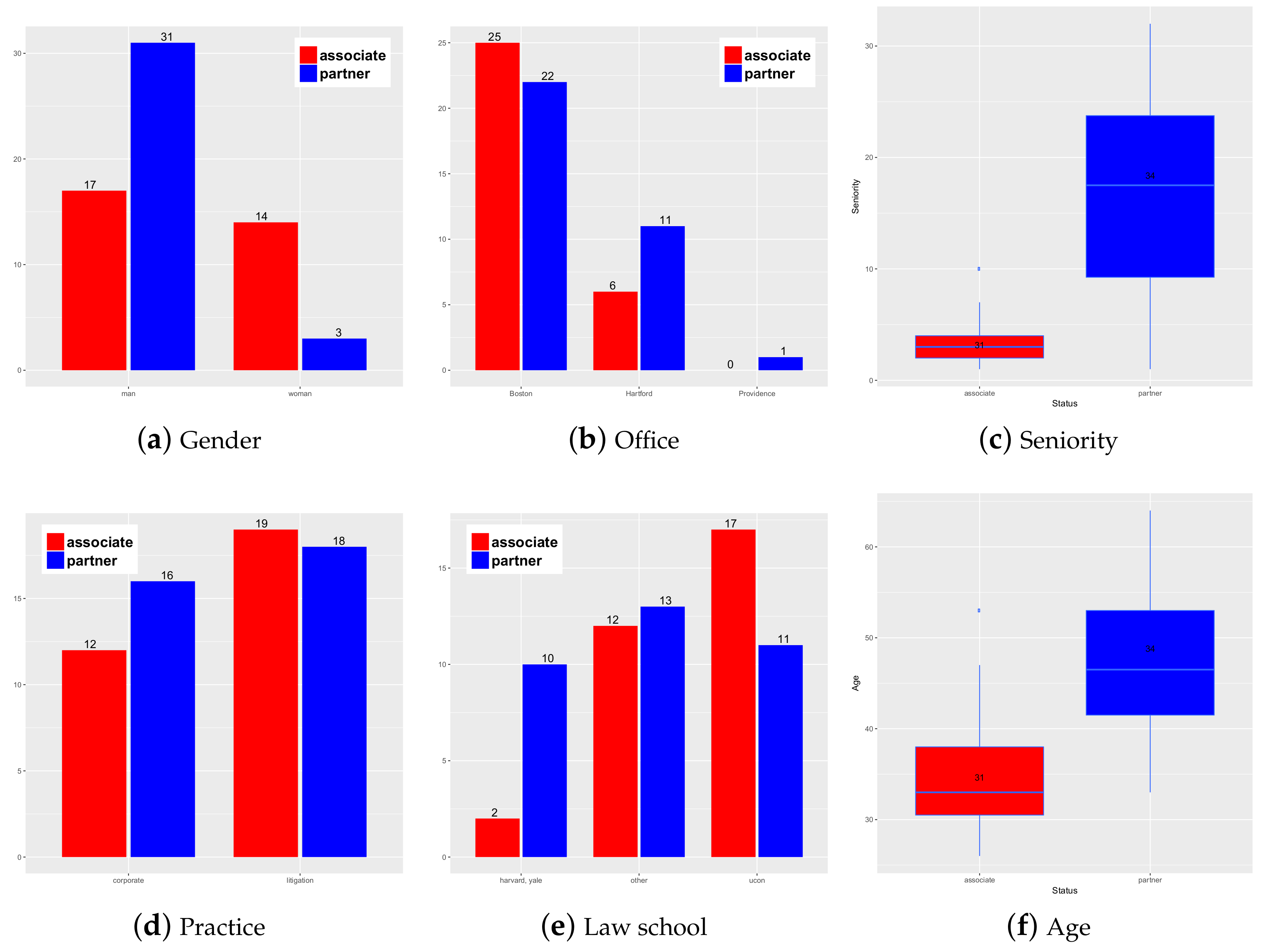
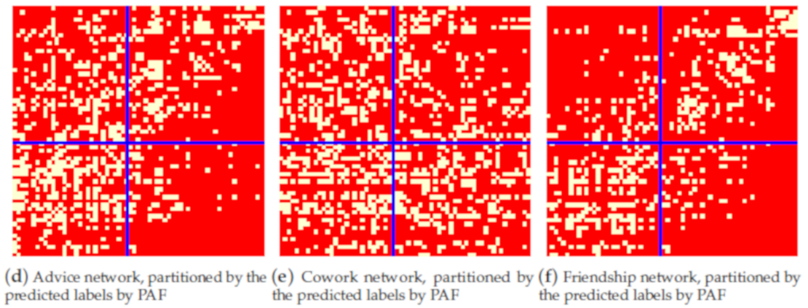
Intuitively, all these three network layers and six attributes can contribute to the community detection task with the ground truth label “status”. Specifically, the descriptive analysis results in Figure 3 present that all these six attributes can provide useful information to distinguish the two values of “status”; the top three panels of Figure 4, i.e., the heatmap plots of the three adjacent matrices partitioned by the ground truth labels, partly present block structure according to the two values of “status”.
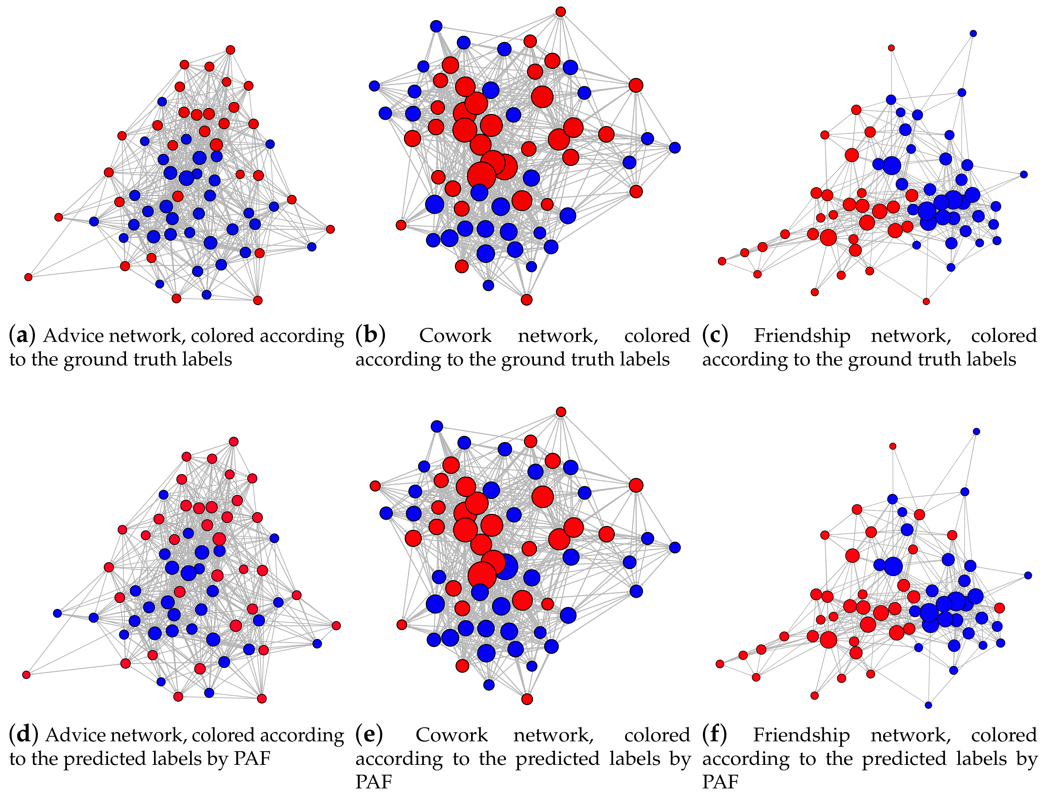
The authors of [45] offered a comparison of seven methods for community detection of this dataset, we recall the NMI results of these methods in [45] by Table 1, together with the NMI result obtained by applying the proposed PAF method to the multi-layer attributed network with m * = 3 network layers and p = 6 attribute variables. Table 1 indicates that the NMI performance of the PAF method is almost the same as the best existing one. Intuitively, the heatmap plots of the three adjacent matrices partitioned by the predicted labels of the PAF method are given in the bottom three panels of Figure 4, which are quite similar to those partitioned by the ground truth labels. Viewed from another perspective, we present the plots of the three network layers, colored by the ground truth labels and the predicted labels by PAF, respectively, in Figure 5, which indicate that the partition by both the ground truth labels and the predicted labels by the proposed PAF method can present a strong assortative structure for the three network layers, especially for the friendship layer. These results demonstrate the practicability of the PAF method in community detection of multi-layer attributed networks.

7. Conclusions

We have proposed PAF—a unified framework and algorithm that is applicable to community detection of multi-layer attributed networks—as well as its special cases, such as single networks, attributed networks, and multi-layer networks. The main idea of PAF is replacing the community label matrix at two different positions in the original objective function with two different substitution matrices, penalizing the gap between the two substitution matrices, and then alternately optimizing each of the substitution matrices as well as some other variable matrices. The results of the simulation study and empirical analysis demonstrate the advantages of the PAF algorithm in community discovery accuracy and compatibility with multiple types of network-related data.
In our future work, we will study community detection of multi-layer attributed networks in statistical ways, where likelihood functions under some statistical models of multi-layer attributed networks will be considered.

Author Contributions

Conceptualization, B.L.; methodology, B.L.; software, J.W.; validation, J.W.; formal analysis, J.L.; investigation, J.W.; resources, J.L.; data curation, J.W.; writing—original draft preparation, J.W.; writing—review and editing, B.L.; visualization, J.W.; supervision, J.L.; project administration, B.L.; funding acquisition, B.L. All authors have read and agreed to the published version of the manuscript.

Funding

The authors gratefully acknowledge Special Fund for Key Laboratories of Jilin Province (20190201285JC), Jilin Provincial Department of Education (JJKH20190293KJ) and Jilin Provincial Science and Technology Development Plan funded Project (20180520026JH).

Conflicts of Interest

The authors declare no conflicts of interest.

Abbreviations

The following abbreviations are used in this manuscript:
ANMFasymmetric non-negative matrix factorization
KLKurdyka-Łojasiewicz
NMFnon-negative matrix factorization
NMInormalized mutual information
PAFpenalized alternative factorization
SBMstochastic block model
SCPspectral clustering with perturbations

Appendix A. Proof of Some Theoretical Results

Appendix A.1. Proof of Proposition 1

Proof. 
As H ( Θ ) 0 and { H ( Θ ( t ) ) } t = 1 is a monotone decreasing sequence, there exists a constant δ > 0 such that Θ ( t ) F δ for each t { 1 , 2 , ... } .□

Appendix A.2. Proof of Proposition 2

Proof. 
Let x ( t ) = v e c ( C ( 1 , t ) C ( 1 , t + 1 ) ) . According to Step 2(a) in the PAF algorithm, we obtain
H ( C ( 1 , t ) , C ( 2 , t ) , { S ( m , t ) } m = 1 m * , V ( t ) ) H ( C ( 1 , t + 1 ) , C ( 2 , t ) , { S ( m , t ) } m = 1 m * , V ( t ) ) = C ( 1 ) H ( C ( 1 , t + 1 ) , C ( 2 , t ) , S k , V ( t ) ) , C ( 1 , t ) C ( 1 , t + 1 ) + 2 x ( t ) T m = 1 m * ω m ( S ( m , t ) C ( 2 , t ) T ) T S ( m , t ) C ( 2 , t ) T I k * × k * + ( λ + ν ) I n k * × n k * x ( t ) F 2 2 ( λ + ν ) 2 x ( t ) F 2 = 2 ( λ + ν ) 2 C ( 1 , t ) C ( 1 , t + 1 ) F 2 .
Similarly, let y ( t ) = vec ( C ( 2 , t + 1 ) C ( 2 , t ) ) , then according Step 2(b) in the PAF algorithm, we have
H ( C ( 1 , t + 1 ) , C ( 2 , t ) , { S ( m , t ) } m = 1 m * , V ( t ) ) H ( C ( 1 , t + 1 ) , C ( 2 , t + 1 ) , { S ( m , t ) } m = 1 m * , V ( t ) ) = C ( 2 ) H ( C ( 1 , t + 1 ) , C ( 2 , t + 1 ) , { S ( m , t ) } m = 1 m * , V ( t ) ) , C ( 2 , t ) C ( 2 , t + 1 ) + 2 y ( t ) T m = 1 m * ω m ( C ( 1 , t + 1 ) S ( m , t ) ) T C ( 1 , t + 1 ) S ( m , t ) I k * × k * + ( λ + ν ) I n k * × n k * y ( t ) F 2 2 ( λ + ν ) 2 y ( t ) F 2 = 2 ( λ + ν ) 2 C ( 2 , t ) C ( 2 , t + 1 ) F 2 .
From Steps 2(c,d) in the PAF algorithm, we obtain
H ( C ( 1 , t + 1 ) , C ( 2 , t + 1 ) , { S ( m , t ) } m = 1 m * , V ( t ) ) H ( C ( 1 , t + 1 ) , C ( 2 , t + 1 ) , { S ( m , t + 1 ) } m = 1 m * , V ( t ) )
α m = 1 m * S ( m , t + 1 ) S ( m , t ) F 2 , H ( C ( 1 , t + 1 ) , C ( 2 , t + 1 ) , { S ( m , t + 1 ) } m = 1 m * , V ( t ) ) H ( C ( 1 , t + 1 ) , C ( 2 , t + 1 ) , { S ( m , t + 1 ) } m = 1 m * , V ( t + 1 ) ) β V ( t + 1 ) V ( t ) F 2 .
Combining the inequalities (A1)–(A4), we have
H ( Θ ( t ) ) H ( Θ ( t + 1 ) ) 2 ( λ + ν ) 2 ( C ( 1 , t + 1 ) C ( 1 , t ) F 2 + C ( 2 , t + 1 ) C ( 2 , t ) F 2 ) + α m = 1 m * S ( m , t + 1 ) S ( m , t ) F 2 + β V ( t + 1 ) V ( t ) F 2 ,
which implies that
ρ 1 Θ ( t ) Θ ( t + 1 ) F 2 H ( Θ ( t ) ) H ( Θ ( t + 1 ) ) ,
where ρ 1 = min { 2 ( λ + ν ) 2 , α , β } .□

Appendix A.3. Proof of Proposition 3

Proof. 
We will first analyze the boundness of C ( 1 ) H ( C ( 1 , t + 1 ) , C ( 2 , t + 1 ) , { S ( m , t + 1 ) } m = 1 m * , V ( t + 1 ) ) . It is easy to check that
C ( 1 ) H ( C ( 1 , t + 1 ) , C ( 2 , t + 1 ) , { S ( m , t + 1 ) } m = 1 m * , V ( t + 1 ) ) = 2 m = 1 m * ω m ( C ( 1 , t + 1 ) S ( m , t + 1 ) C ( 2 , t + 1 ) T A ( m ) ) ( S ( m , t + 1 ) C ( 2 , t + 1 ) T ) T + 2 λ ( C ( 1 , t + 1 ) C ( 2 , t + 1 ) ) + ω 0 ( C ( 1 , t + 1 ) V ( t + 1 ) T X ) V ( t + 1 ) + 2 ν C ( 1 , t + 1 ) .
According to Step 2(a) in the PAF algorithm, we know
C ( 1 ) H ( C ( 1 , t + 1 ) , C ( 2 , t ) , { S ( m , t ) } m = 1 m * , V ( t ) ) = 2 m = 1 m * ω m ( C ( 1 , t + 1 ) S ( m , t ) C ( 2 , t ) T A ( m ) ) ( S ( m , t ) C ( 2 , t ) T ) T + 2 λ ( C ( 1 , t + 1 ) C ( 2 , t ) ) + ω 0 ( C ( 1 , t + 1 ) V ( t ) T X ) V ( t ) + 2 ν C ( 1 , t + 1 ) = 0 .
Together with (A6) and (A7), we have
C ( 1 ) H ( C ( 1 , t + 1 ) , C ( 2 , t + 1 ) , { S ( m , t + 1 ) } m = 1 m * , V ( t + 1 ) ) F 2 m = 1 m * ω m C ( 1 , t + 1 ) S ( m , t + 1 ) C ( 2 , t + 1 ) T ) ( S ( m , t + 1 ) C ( 2 , t ) T ) T C ( 1 , t + 1 ) S ( m , t ) C ( 2 , t ) T ( S ( m , t ) C ( 2 , t ) T ) T F + 2 m = 1 m * ω m A ( m ) ( ( S ( m , t + 1 ) C ( 2 , t + 1 ) T ) T ( S ( m , t ) C ( 2 , t ) T ) T ) F + 2 λ C ( 2 , t + 1 ) C ( 2 , t ) F + ω 0 C ( 1 , t + 1 ) ( V ( t + 1 ) T V ( t + 1 ) V ( t ) T V ( t ) ) F + 2 ω 0 X ( V ( t + 1 ) V ( t ) ) F 2 C ( 1 , t + 1 ) F m = 1 m * ω m ( ( S ( m , t + 1 ) S ( m , t ) ) C ( 2 , t + 1 ) T ( S ( m , t + 1 ) C ( 2 , t + 1 ) T ) T F + S ( m , t ) ( C ( 2 , t + 1 ) C ( 2 , t ) ) T ( S ( m , t + 1 ) C ( 2 , t + 1 ) T ) T F + S ( m , t ) C ( 2 , t ) T C ( 2 , t + 1 ) ( S ( m , t + 1 ) S ( m , t ) ) T F + S ( m , t ) C ( 2 , t ) T ( C ( 2 , t + 1 ) C ( 2 , t ) ) S ( m , t ) T F ) + 2 m = 1 m * ω m [ A ( m ) F ( C ( 2 , t + 1 ) C ( 2 , t ) ) S ( m , t + 1 ) T F + A ( m ) F C ( 2 , t ) ( S ( m , t + 1 ) S ( m , t ) ) T F ] + 2 λ C ( 2 , t + 1 ) C ( 2 , t ) F + ω 0 C ( 1 , t + 1 ) ( V ( t + 1 ) T V ( t + 1 ) V ( t ) T V ( t ) ) F + ω 0 X ( V ( t + 1 ) V ( t ) ) F 2 δ ( 2 δ 3 + τ ) m = 1 m * S ( m , t + 1 ) S ( m , t ) F + ( 2 δ 4 + 2 τ δ m * + 2 λ ) C ( 2 , t + 1 ) C ( 2 , t ) F + ( 2 δ 2 + X F ) V ( t + 1 ) V ( t ) F ,
where τ = max { A ( 1 ) F , A ( 2 ) F , ... , A ( m * ) F } .
Next, we see that
C ( 2 ) H ( C ( 1 , t + 1 ) , C ( 2 , t + 1 ) , { S ( m , t + 1 ) } m = 1 m * , V ( t + 1 ) ) = 2 m = 1 m * ω m ( C ( 1 , t + 1 ) S ( m , t + 1 ) ) T ( C ( 1 , t + 1 ) S ( m , t + 1 ) C ( 2 , t + 1 ) T A ) + 2 λ ( C ( 2 , t + 1 ) C ( 1 , t + 1 ) ) + ω 0 ( C ( 2 , t + 1 ) V ( t + 1 ) T X ) V ( t + 1 ) + 2 ν C ( 2 , t + 1 ) ,
and from Step 2(b) in the PAF algorithm,
C ( 2 ) H ( C ( 1 , t + 1 ) , C ( 2 , t + 1 ) , { S ( m , t ) } m = 1 m * , V ( t ) ) = 2 m = 1 m * ω m ( C ( 1 , t + 1 ) S ( m , t ) ) T ( C ( 1 , t + 1 ) S ( m , t ) C ( 2 , t + 1 ) T A ) + 2 λ ( C ( 2 , t + 1 ) C ( 1 , t + 1 ) ) + ω 0 ( C ( 2 , t + 1 ) V ( t ) T X ) V ( t ) + 2 ν C ( 2 , t + 1 ) = 0 .
As a result,
C ( 2 ) H ( C ( 1 , t + 1 ) , C ( 2 , t + 1 ) , { S ( m , t + 1 ) } m = 1 m * , V ( t + 1 ) ) F 2 C ( 2 , t + 1 ) F m = 1 m * ω m ( C ( 1 , t + 1 ) S ( m , t + 1 ) ) T C ( 1 , t + 1 ) S ( m , t + 1 ) ( C ( 1 , t + 1 ) S ( m , t ) ) T C ( 1 , t + 1 ) S ( m , t ) F + 2 m = 1 m * ω m ( S ( m , t + 1 ) C ( 1 , t + 1 ) S ( m , t ) C ( 1 , t + 1 ) ) A ( m ) T F + ω 0 X F V ( t + 1 ) V ( t ) F + ω 0 C ( 2 , t + 1 ) F V ( t + 1 ) V ( t + 1 ) T V ( t ) V ( t ) T F 2 m = 1 m * ω m ( C ( 2 , t + 1 ) F S ( m , t + 1 ) C ( 1 , t + 1 ) T C ( 1 , t + 1 ) F S ( m , t + 1 ) S ( m , t ) F + S ( m , t + 1 ) S ( m , t ) F C ( 2 , t + 1 ) F C ( 1 , t + 1 ) T C ( 1 , t + 1 ) S ( m ) , k F ) + 2 m = 1 m * ω m ( S ( m , t + 1 ) S ( m , t ) ) F C ( 1 , t + 1 ) F A ( m ) F + ω 0 C ( 1 , t + 1 ) F V ( t + 1 ) F V ( t + 1 ) V ( t ) F + ω 0 C ( 2 , t + 1 ) F V ( t ) F V ( t + 1 ) V ( t ) F + ω 0 X F V ( t + 1 ) V ( t ) F 2 δ ( 2 δ 3 + τ ) m = 1 m * S ( m , t + 1 ) S ( m , t ) F + ( 2 δ 2 + X F ) V ( t + 1 ) V ( t ) F .
Similarly, we have
S ( m ) H ( C ( 1 , t + 1 ) , C ( 2 , t + 1 ) , { S ( m , t + 1 ) } m = 1 m * , V ( t + 1 ) ) F 2 α ( S ( m , t + 1 ) S ( m , t ) ) F
and
V H ( C ( 1 , t + 1 ) , C ( 2 , t + 1 ) , { S ( m , t + 1 ) } m = 1 m * , V ( t + 1 ) ) F 2 β ( V ( t + 1 ) V ( t ) ) F .
According to (A8) and (A11)–(A13), we finally obtain that
H ( Θ ( t + 1 ) ) F ρ 2 Θ ( t + 1 ) Θ ( t ) F ,
where ρ 2 = max { 4 δ ( 2 δ 3 + τ ) + 2 α , 2 ( δ 4 + τ δ m * + λ ) , 2 ( 2 δ 2 + X F + β ) } .

Appendix A.4. Proof of Theorem 1

To establish the proof of Theorem 1, we need to recall the definition of Kurdyka-Łojasiewicz (KL) property and prove the following two properties.
  • Sufficient decrease property:
    ρ 1 > 0 , such that ρ 1 Θ ( t + 1 ) Θ ( t ) F 2 [ H ( Θ ( t ) ) H ( Θ ( t + 1 ) ) ] ;
  • A subgradient lower bound for the iteration gap:
    ρ 2 > 0 , t { 0 , 1 , ... } and κ ( t + 1 ) H ( Θ ( t + 1 ) ) : κ ( t + 1 ) F ρ 2 Θ ( t + 1 ) Θ ( t ) F ,
    where H is the subderivative of the function H and
    Θ = ( C ( 1 ) , C ( 2 ) , { S ( m ) } m = 1 m * , V ) , H ( Θ ) = m = 1 m * ω m A ( m ) C ( 1 ) S ( m ) C ( 2 ) F 2 + ω 0 2 l = 1 2 X C ( l ) V T F 2 + λ C ( 1 ) C ( 2 ) F 2 + ν { C ( 1 ) F 2 + C ( 2 ) F 2 + V F 2 + m = 1 m * S ( m ) F 2 } , H ( Θ ) = C ( 1 ) H ( Θ ) , C ( 2 ) H ( Θ ) , S ( 1 ) H ( Θ ) , ... , S ( m * ) H ( Θ ) , V H ( Θ ) .
Definition A1. 
(KL property [58,59]) Let σ : R d ( , + ] be a proper lower semicontinuous function. For x ¯ dom σ { x R d : σ ( x ) } if there exists an η ( 0 , + ] , a neighborhood Γ of x ¯ and a function ξ Φ η , such that for all x X { y R d : σ ( x ¯ ) < σ ( y ) < σ ( x ¯ ) + η } the following inequality holds
ξ σ ( u ) σ ( x ¯ ) dist 0 , σ ( x ) 1 ,
then σ is said to have the KL property at x ¯ . σ is called a KL function, if σ satisfies the KL property at each point in dom σ .
Here, dist ( x , X ) denotes the shortest distance between the point x and the point set X , i.e., dist ( x , X ) = min y X dist ( x , y ) , and Φ η denotes the class of all concave and continuous functions ξ : [ 0 , η ) R + , η R + , which satisfies: a ) ξ ( 0 ) = 0 ; b ) ξ is continuous differentiable on ( 0 , η ) ; c ) for all s ( 0 , η ) , ξ ( s ) > 0 .
Now, we are ready to present the proof of Theorem 1, based on the fact that the function H is a KL function.
Proof. 
Suppose that Θ ¯ is the limit point of a sub-sequence { Θ ( t i ) } , i.e., lim i + Θ ( t i ) = Θ ¯ . It is clear that the function H is continuous w.r.t. Θ , therefore
lim i + H ( Θ ( t i ) ) = H ( Θ ¯ ) .
Note that H ( Θ ( t ) ) is monotonically non-increasing and then converges to H ( Θ ¯ ) .
From Propositions 2 and 3, we obtain that H ( Θ ( t ) ) 0 as t . Then we obtain 0 H ( Θ ¯ ) , i.e., Θ ¯ is a critical point of Φ . Let Ω be the set of all limit points of subsequences of { Θ ( t ) } t = 1 , we then know that
d i s t ( Θ ( t ) , Ω ) 0 , a s t .
Accordingly, from (A18) and (A19), we obtain that for any γ > 0 , ϵ > 0 , there exists an integer t u > 0 such that for all t > t u ,
H ( Θ ( t ) ) < H ( Θ ¯ ) + γ a n d d i s t ( Θ ( t ) , Ω ) < ϵ .
It is known that the function H is a KL function [59], then by using the KL inequality in Definition (A1) and (A20), there exist ξ , such that
ξ ( H ( Θ ( t ) ) H ( Θ ¯ ) ) d i s t ( 0 , H ( Θ ( t ) ) ) 1 .
According to Proposition 3, we have
ξ ( H ( Θ ( t ) ) H ( Θ ¯ ) ) 1 ρ 2 Θ ( t ) Θ ( t 1 ) F .
Besides, ξ is concave and we have that
ξ ( H ( Θ ( t ) ) H ( Θ ¯ ) ) ξ ( H ( Θ ( t + 1 ) ) H ( Θ ¯ ) ) ξ ( H ( Θ ( t ) ) H ( Θ ¯ ) ) ( H ( Θ ( t ) ) H ( Θ ( t + 1 ) ) ) .
For convenience, let
Δ t , t + 1 = ξ ( H ( Θ ( t ) ) H ( Θ ¯ ) ) ξ ( H ( Θ ( t + 1 ) ) H ( Θ ¯ ) )
Then according to propositions 2 and 3, we have
Δ t , t + 1 ρ 1 Θ ( t + 1 ) Θ ( t ) F 2 ρ 2 Θ ( t ) Θ ( t 1 ) F
i.e.,
4 Θ ( t + 1 ) Θ ( t ) F 2 4 ρ 2 ρ 1 Δ t , t + 1 Θ ( t ) Θ ( t 1 ) F ( ρ 2 ρ 1 Δ t , t + 1 + Θ ( t ) Θ ( t 1 ) F ) 2 ,
which indicates that
2 Θ ( t + 1 ) Θ ( t ) F Θ ( t ) Θ ( t 1 ) F + ρ 2 ρ 1 Δ t , t + 1 .
Summing up (A24) over t from 1 to z and then yields the following inequality,
2 t = 1 z Θ ( t + 1 ) Θ ( t ) F t = 1 z Θ ( t ) Θ ( t 1 ) F + ρ 2 ρ 1 t = 1 z Δ t , t + 1 t = 1 z Θ ( t + 1 ) Θ ( t ) F + Θ ( 1 ) Θ ( 0 ) F + ρ 2 ρ 1 Δ 1 , z + 1
i.e.,
t = 1 z Θ ( t + 1 ) Θ ( t ) F < Θ ( 1 ) Θ ( 0 ) F + ρ 2 ρ 1 ξ ( H ( Θ ( 1 ) ) H ( Θ ¯ ) ) .
We take limits on the left side of inequality of (A26) as z and get
t = 1 + Θ ( t ) Θ ( t + 1 ) F Θ ( 1 ) Θ ( 0 ) F + ρ 2 ρ 1 ξ ( H ( Θ ( 1 ) ) H ( Θ ¯ ) ) < + .
It is easy to know that (A27) implies that { Θ ( t ) } t = 1 is a Cauchy sequence, and thus is a convergent sequence and this completes the proof, i.e., the sequence { Θ ( t ) } t = 1 converges to a critical point of H in (A17).□

Appendix B. Some Additional Numerical Results

In this section, we mainly investigate the computational efficiency of the proposed algorithm for relatively large scale multi-layer attributed networks via some additional numerical results. We consider the following simulation setting for multi-layer networks and multi-layer attributed networks.
V
The m * = 3 n × n adjacent matrices { A ( 1 ) , A ( 2 ) , A ( 3 ) } are generated independently from the undirected and directed multi-layer SBMs, respectively, with common community labels, where the parameters are set as follows,
P 1 = 0 . 2 0 . 2 0 . 13 0 . 2 0 . 2 0 . 13 0 . 13 0 . 13 0 . 2 , P 2 = 0 . 8 0 . 2 0 . 13 0 . 13 0 . 13 0 . 2 0 . 2 0 . 13 0 . 2 0 . 2 , P 3 = 0 . 8 0 . 2 0 . 13 0 . 2 0 . 13 0 . 2 0 . 13 0 . 2 0 . 13 0 . 2 , π = 0 . 3 3 ˙ 0 . 3 3 ˙ 0 . 3 3 ˙ .
Each row of the n × 3 attribution matrix is independently generated from the multivariate normal distribution N 3 ( μ k , σ 2 I 3 ) , where the kth element of μ k is 1 and the remaining elements are 0, and σ 2 = 0 . 08 .
As suggested in Figure A1, the proposed algorithm framework is compatible with a variety of network related data, has relatively good accuracy of community discovery and acceptable computational efficiency. Compared with the algorithm SCP, which provides initial value for the proposed algorithm, the proposed algorithm does not excessively reduce the computational efficiency.
Figure A1. The left two panels present the NMI results for Setting V and the right two panels present the RT (running time in log-second) results for Setting V.
Mathematics 08 00239 g0a1

References

  1. Newman, M.E.J. Networks; Oxford University Press: Oxford, UK, 2018. [Google Scholar]
  2. Wasserman, S. Advances in Social Network Analysis: Research in the Social and Behavioral Sciences; Sage: Thousand Oaks, CA, USA, 1994. [Google Scholar]
  3. Bader, G.D.; Hogue, C.W.V. An automated method for finding molecular complexes in large protein interaction networks. BMC Bioinform. 2003, 4, 2. [Google Scholar] [CrossRef] [Green Version]
  4. Sporns, O. Networks of the Brain; MIT Press: Cambridge, MA, USA, 2010. [Google Scholar]
  5. Rogers, E.M.; Kincaid, D.L. Communication Networks: Toward a New Paradigm for Research; Free Press: New York, NY, USA, 1981; Volume 11, p. 2. [Google Scholar]
  6. Schlitt, T.; Brazma, A. Current approaches to gene regulatory network modelling. BMC Bioinform. 2007, 8, S9. [Google Scholar] [CrossRef] [Green Version]
  7. Mcpherson, M.; Smithlovin, L.; Cook, J.M. Birds of a feather: Homophily in social networks. Rev. Sociol. 2001, 27, 415–444. [Google Scholar] [CrossRef] [Green Version]
  8. Moody, J.; White, D.R. Structural cohesion and embeddedness: A hierarchical concept of social groups. Am. Sociol. Rev. 2003, 103–127. [Google Scholar] [CrossRef] [Green Version]
  9. Flake, G.W.; Lawrence, S.; Giles, C.L. Efficient identification of web communities. In Proceedings of the Sixth ACM SIGKDD International Conference on Knowledge Discovery and Data Mining, Boston, MA, USA, 20–23 August 2000; pp. 150–160. [Google Scholar]
  10. Sporns, O.; Betzel, R.F. Modular brain networks. Annu. Rev. Psychol. 2016, 67, 613–640. [Google Scholar] [CrossRef] [PubMed] [Green Version]
  11. Spirin, V.; Mirny, L.A. Protein complexes and functional modules in molecular networks. Proc. Natil. Acad. Sci. USA 2003, 100, 12123–12128. [Google Scholar] [CrossRef] [Green Version]
  12. Fortunato, S. Community detection in graphs. Phys. Rep. 2010, 10, 75–174. [Google Scholar] [CrossRef] [Green Version]
  13. Fortunato, S.; Hric, D. Community detection in networks: A user guide. Phys. Rep. 2016, 659, 1–44. [Google Scholar] [CrossRef] [Green Version]
  14. Khan, B.S.; Niazi, M.A. Network community detection: A review and visual survey. arXiv 2017, arXiv:1708.00977. [Google Scholar]
  15. Porter, M.A.; Onnela, J.-P.; Mucha, P.J. Communities in networks. Not. AMS 2009, 56, 1082–1097. [Google Scholar]
  16. Schaub, M.T.; Delvenne, J.-C.; Rosvall, M.; Lambiotte, R. The many facets of community detection in complex networks. Appl. Netw. Sci. 2017, 2, 4. [Google Scholar] [CrossRef] [PubMed] [Green Version]
  17. Newman, M.E.J. Detecting community structure in networks. Eur. Phys. J. B 2004, 38, 321–330. [Google Scholar] [CrossRef]
  18. Hespanha, J.P. An Efficient Matlab Algorithm for Graph Partitioning; University of California: Santa Barbara, CA, USA, 2004. [Google Scholar]
  19. Shi, J.; Malik, J. Normalized cuts and image segmentation. IEEE Trans. Pattern Anal. Mach. Intell. 2000, 22, 888–905. [Google Scholar]
  20. Newman, M.E.J.; Girvan, M. Finding and evaluating community structure in networks. Phys. Rev. E 2004, 69, 026113. [Google Scholar] [CrossRef] [PubMed] [Green Version]
  21. Jin, J. Fast community detection by score. Ann. Stat. 2015, 43, 57–89. [Google Scholar] [CrossRef]
  22. Lei, J.; Rinaldo, A. Consistency of spectral clustering in stochastic block models. Ann. Stat. 2015, 43, 215–237. [Google Scholar] [CrossRef]
  23. McSherry, F. Spectral partitioning of random graphs. In Proceedings of the 42nd IEEE Symposium on Foundations of Computer Science, Newport Beach, CA, USA, 8–11 October 2001; pp. 529–537. [Google Scholar]
  24. Rohe, K.; Chatterjee, S.; Yu, B. Spectral clustering and the high-dimensional stochastic blockmodel. Ann. Stat. 2011, 39, 1878–1915. [Google Scholar] [CrossRef] [Green Version]
  25. Cai, T.T.; Li, X. Robust and computationally feasible community detection in the presence of arbitrary outlier nodes. Ann. Stat. 2015, 43, 1027–1059. [Google Scholar] [CrossRef] [Green Version]
  26. Hajek, B.; Wu, Y.; Xu, J. Achieving exact cluster recovery threshold via semidefinite programming: Extensions. IEEE Trans. Inf. Theory 2016, 62, 5918–5937. [Google Scholar] [CrossRef] [Green Version]
  27. Le, C.M.; Levina, E.; Vershynin, R. Optimization via low-rank approximation for community detection in networks. Ann. Stat. 2016, 44, 373–400. [Google Scholar] [CrossRef]
  28. Wang, F.; Li, T.; Wang, X.; Zhu, S.; Ding, C. Community discovery using non-negative matrix factorization. Data Min. Knowl. Discov. 2011, 22, 493–521. [Google Scholar] [CrossRef]
  29. Holland, P.W.; Laskey, K.B.; Leinhardt, S. Stochastic block models: First steps. Soc. Netw. 1983, 5, 109–137. [Google Scholar] [CrossRef]
  30. Karrer, B.; Newman, M.E.J. Stochastic blockmodels and community structure in networks. Phys. Rev. E 2011, 83, 016107. [Google Scholar] [CrossRef] [Green Version]
  31. Hoff, P.D. Modeling homophily and stochastic equivalence in symmetric relational data. In Advances in Neural Information Processing Systems; Neural Information Processing Systems Foundation, Inc.: La Jolla, CA, USA, 2008; pp. 657–664. [Google Scholar]
  32. Newman, M.E.J. Modularity and community structure in networks. Proc. Natl. Acad. Sci. USA 2006, 103, 8577–8582. [Google Scholar] [CrossRef] [PubMed] [Green Version]
  33. Amini, A.A.; Chen, A.; Bickel, P.J.; Levina, E. Pseudo-likelihood methods for community detection in large sparse networks. Ann. Stat. 2013, 41, 2097–2122. [Google Scholar] [CrossRef]
  34. Qin, T.; Rohe, K. Regularized spectral clustering under the degree-corrected stochastic blockmodel. In Advances in Neural Information Processing Systems; Neural Information Processing Systems Foundation, Inc.: La Jolla, CA, USA, 2013; pp. 3120–3128. [Google Scholar]
  35. Hoff, P.D. Random effects models for network data. In Dynamic Social Network Modeling and Analysis Workshop Summary and Papers; National Academies Press: Washington, DC, USA, 2003. [Google Scholar]
  36. Zanghi, H.; Volant, S.; Ambroise, C. Clustering based on random graph model embedding vertex features. Pattern Recogn. Lett. 2010, 31, 830–836. [Google Scholar] [CrossRef] [Green Version]
  37. Handcock, M.S.; Raftery, A.E.; Tantrum, J.M. Model-based clustering for social networks. J. R. Stat. Soc. Ser. A (Stat. Soc.) 2007, 170, 301–354. [Google Scholar] [CrossRef] [Green Version]
  38. Yang, T.; Jin, R.; Chi, Y.; Zhu, S. Combining link and content for community detection: A discriminative approach. In Proceedings of the 15th ACM SIGKDD International Conference on Knowledge Discovery and Data Mining, Paris, France, 28 June–1 July 2009; pp. 927–936. [Google Scholar]
  39. Kim, M.; Leskovec, L.J. Latent multi-group membership graph model. arXiv 2012, arXiv:1205.4546. [Google Scholar]
  40. Leskovec, J.; Mcauley, J.J. Learning to discover social circles in ego networks. In Advances in Neural Information Processing Systems; Neural Information Processing Systems Foundation, Inc.: La Jolla, CA, USA, 2012; pp. 539–547. [Google Scholar]
  41. Yang, J.; McAuley, J.; Leskovec, J. Community detection in networks with node attributes. In Proceedings of the 2013 IEEE 13th International Conference on Data Mining, Dallas, TX, USA, 7–10 December 2013; pp. 1151–1156. [Google Scholar]
  42. Xu, Z.; Ke, Y.; Wang, Y.; Cheng, H.; Cheng, J. A model-based approach to attributed graph clustering. In Proceedings of the 2012 ACM SIGMOD International Conference on Management of Data, Dallas, TX, USA, 16–18 May 2000; pp. 505–516. [Google Scholar]
  43. Hoang, T.-A.; Lim, E.-P. On joint modeling of topical communities and personal interest in microblogs. In International Conference on Social Informatics; Springer: Cham, Switzerland, 2014; pp. 1–16. [Google Scholar]
  44. Newman, M.E.J.; Clauset, A. Structure and inference in annotated networks. Nat. Commun. 2016, 7, 11863. [Google Scholar] [CrossRef] [Green Version]
  45. Zhang, Y.; Levina, E.; Zhu, J. Community detection in networks with node features. Electron. J. Stat. 2016, 10, 3153–3178. [Google Scholar] [CrossRef]
  46. Boorman, S.A.; White, H.C. Social structure from multiple networks. ii. role structures. Am. J. Sociol. 1976, 81, 1384–1446. [Google Scholar] [CrossRef]
  47. Breiger, R.L. Social structure from multiple networks. Am. J. Sociol. 1976, 81, 730–780. [Google Scholar]
  48. Cheng, W.; Zhang, X.; Guo, Z.; Wu, Y.; Sullivan, P.F.; Wang, W. Flexible and robust co-regularized multi-domain graph clustering. Knowl. Discov. Data Min. 2013, 320–328. [Google Scholar]
  49. Boccaletti, S.; Bianconi, G.; Criado, R.; DelGenio, C.I.; Gómez-Gardenes, J.; Romance, M.; Sendina-Nadal, I.; Wang, Z.; Zanin, M. The structure and dynamics of multilayer networks. Phys. Rep. 2014, 544, 1–122. [Google Scholar] [CrossRef] [Green Version]
  50. Kivelä, M.; Arenas, A.; Barthelemy, M.; Gleeson, J.P.; Moreno, Y.; Porter, M.A. Multilayer networks. J. Complex Netw. 2014, 2, 203–271. [Google Scholar]
  51. Matias, C.; Miele, V. Statistical clustering of temporal networks through a dynamic stochastic block model. J. R. Stat. Soc. Ser. B (Stat. Methodol.) 2017, 79, 1119–1141. [Google Scholar] [CrossRef]
  52. Cardillo, A.; Gómez-Gardenes, J.; Zanin, M.; Romance, M.; Papo, D.; DelPozo, F.; Boccaletti, S. Emergence of network features from multiplexity. Sci. Rep. 2013, 3, 1344. [Google Scholar] [CrossRef] [Green Version]
  53. Fienberg, S.E.; Meyer, M.M.; Wasserman, S.S. Analyzing Data from Multivariate Directed Graphs: An Application to Social Networks; Technical Report; Department of Statistics, Carnegie Mellon University: Pittsburgh, PA, USA, 1980. [Google Scholar]
  54. Fienberg, S.E.; Meyer, M.M.; Wasserman, S.S. Statistical analysis of multiple sociometric relations. J. Am. Stat. Assoc. 1985, 80, 51–67. [Google Scholar] [CrossRef]
  55. Ferriani, S.; Fonti, F.; Corrado, R. The social and economic bases of network multiplexity: Exploring the emergence of multiplex ties. Strateg. Organ. 2013, 11, 7–34. [Google Scholar] [CrossRef]
  56. Yan, T.; Jiang, B.; Fienberg, E.S.; Leng, C. Statistical inference in a directed network model with covariates. J. Am. Stat. Assoc. 2019, 114, 857–868. [Google Scholar] [CrossRef] [Green Version]
  57. Lazega, E. The Collegial Phenomenon: The Social Mechanisms of Cooperation among Peers in a Corporate Law Partnership; Oxford University Press on Demand: Oxfor, UK, 2001. [Google Scholar]
  58. Attouch, H.; Bolte, J.; Svaiter, B.F. Convergence of descent methods for semi-algebraic and tame problems: proximal algorithms, forward-backward splitting, and regularized gauss-seidel methods. Math. Programm. 2013, 137, 91–129. [Google Scholar] [CrossRef]
  59. Bolte, J.; Sabach, S.; Teboulle, M. Proximal alternating linearized minimization for nonconvex and nonsmooth problems. Math. Programm. 2014, 146, 459–494. [Google Scholar] [CrossRef]
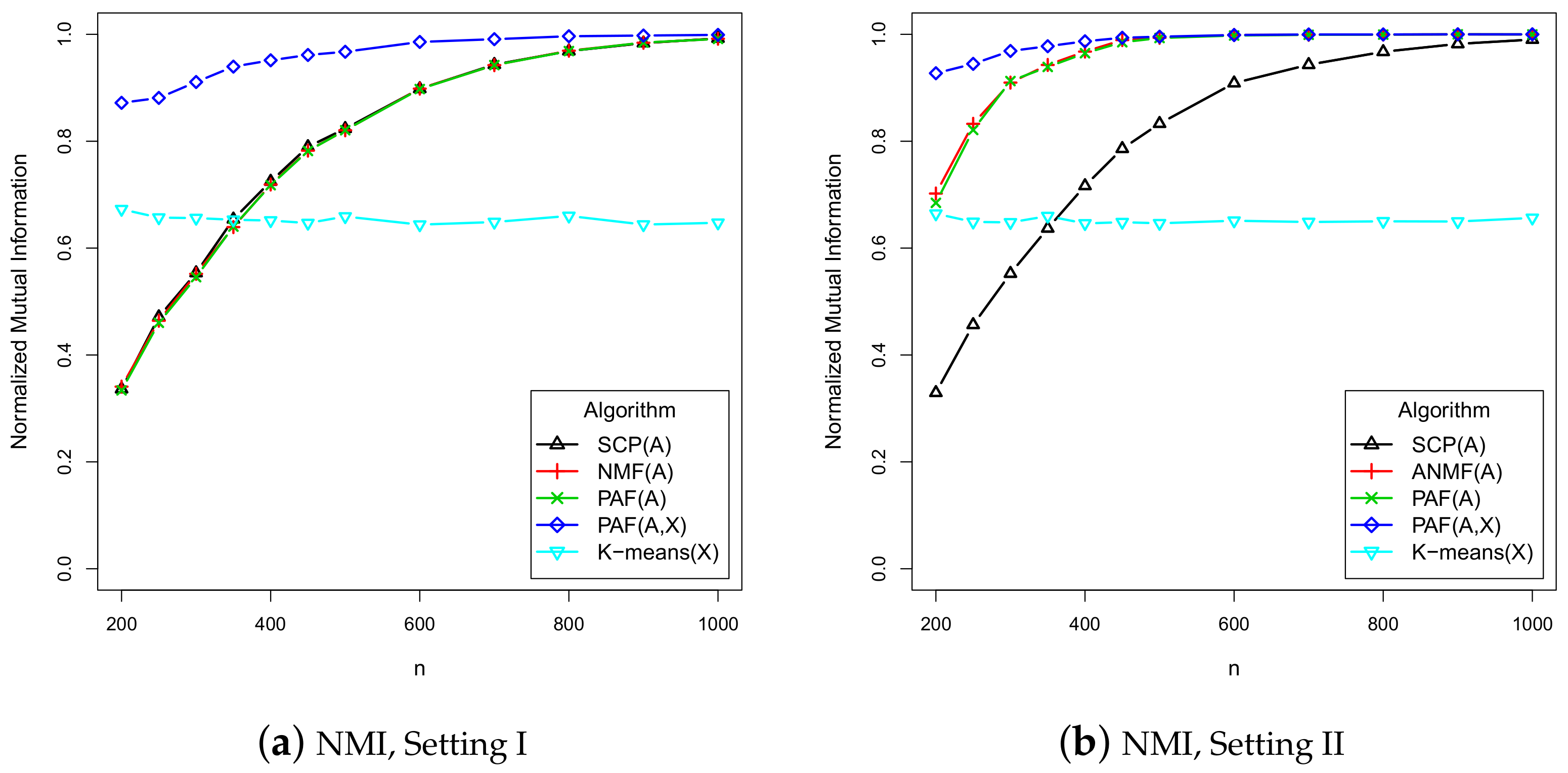
Figure 1. The two panels present the NMI results for Setting I (undirected SBM) and Setting II (directed SBM), respectively.
Mathematics 08 00239 g001
Figure 2. The two panels present the NMI results for Setting III (undirected multi-layer SBM) and Setting IV (directed multi-layer SBM), respectively.
Mathematics 08 00239 g002aMathematics 08 00239 g002b
Figure 3. The left four panels are the grouped bar charts of status versus the four categorical features: “gender”, “office”, “practice”, and “law school”. The right two panels are the box-plots of “status” versus the two count variables “seniority” and “age”.
Mathematics 08 00239 g003
Figure 4. Heatmap plots of the adjacent matrices of the three network layers, ordered by the ground truth labels and the predicted labels by PAF, respectively.
Mathematics 08 00239 g004aMathematics 08 00239 g004b
Figure 5. Plots of the three network layers, colored by the ground truth labels and the predicted labels by PAF, respectively.
Mathematics 08 00239 g005
Table 1. The NMI results of eight community detection methods for the multi-layer attributed network with m * = 3 network layers and p = 6 attribute variables.
MethodNMI
JCDC, ω n = 5 0.54
JCDC, ω n = 1 . 5 0.50
SCP0.44
k-means0.44
CASC0.49
CESNA0.07
BAGC0.20
PAF0.58