Multiscale Compression Algorithm for Solving Nonlinear Ill-Posed Integral Equations via Landweber Iteration

Abstract

In this paper, Landweber iteration with a relaxation factor is proposed to solve nonlinear ill-posed integral equations. A compression multiscale Galerkin method that retains the properties of the Landweber iteration is used to discretize the Landweber iteration. This method leads to the optimal convergence rates under certain conditions. As a consequence, we propose a multiscale compression algorithm to solve nonlinear ill-posed integral equations. Finally, the theoretical analysis is verified by numerical results.

1. Introduction

Ill-posed problems [1,2] include linear [3] and nonlinear [4,5,6,7] ill-posed problems. With the development of applied science, studies on nonlinear ill-posed problems are attracting increased attention, and a variety of methods have emerged. Some of the most widely known methods are Tikhonov regularization [8,9,10,11,12,13] and Landweber iteration [14,15,16,17]. The purpose of this study was to explore a compression multiscale Galerkin method for solving nonlinear ill-posed integral equations via Landweber iterations.

Landweber iteration is a regularization method when the iteration is terminated by the generalized discrepancy principle. Hanke et al. [14] used Landweber iteration to solve nonlinear ill-posed problems for the first time, and proved the convergence and convergence rate of the Landweber iteration. However, they did not consider the case of finite dimensions. Based on the gradient method, Neubauer [18] presented a new iterative method that greatly reduces iteration number. The convergence and convergence rate of the new method were proven. Neubauer did not consider the case of finite dimensions either. However, in numerical simulations and practical applications, we should consider regularization methods of finite dimension to solve nonlinear ill-posed problems. For this, Jin and Scherzer provided their results [16,19] in this field. In previous studies [14,16,18,19], the important parameter in the generalized discrepancy principle was greater than two. This is not satisfactory. Hanke [15] derived a smaller parameter for the generalized discrepancy principle that may be close to one under certain conditions. To obtain a better approximation solution, we hope the parameter in the generalized discrepancy principle is as close to one as possible.

From the development of Landweber iteration, the estimate of the parameter in the generalized discrepancy principle depends on an unknown constant, but the selection range of the parameter was not optimal in previous studies [14,16,18,19]. Therefore, the approximate solution obtained by this parameter is also not optimal. To obtain a better approximate solution, this paper introduces the radius $\rho$ of the field and the relaxation factor $\omega$ under the strong Scherzer condition to improve the selection range of the parameter. Simultaneously, by combination with the generalized discrepancy principle, the convergence rates of the Landweber iteration are proven in finite dimensional space in this paper.

This paper is organized as follows. In Section 2, we outline some lemmas and propositions of Landweber iteration under the strong Scherzer condition. In Section 3, we describe the matrix form of the Landweber iteration discretized using the multiscale Galerkin method, and the convergence of the Landweber iteration is proven in finite dimensions. In Section 4, we develop a compression multiscale Galerkin method for Landweber iteration to solve nonlinear ill-posed integral equations, which leads to an optimal approximate solution under certain conditions. A multiscale compression algorithm is proposed to solve nonlinear ill-posed integral equations. Finally, in Section 5, we provide numerical example to verify the theoretical results.

2. Landweber Iteration

In this section, we will describe some lemmas and propositions of Landweber iteration for solving nonlinear integral equations in detail. These results are based on [14,15].

Suppose that $\Omega \subset {\mathbb{R}}^d$ is a bounded domain with $d\ge 1$. Let spaces $\mathbb{X}$ and $\mathbb{Y}$ denote Hilbert spaces. For the sake of simplicity, inner products and norms of Hilbert space are denoted as $⟨·,·⟩$ and $\parallel ·\parallel$, respectively, unless otherwise specified. The nonlinear compact operator $F:\mathbb{X}\to \mathbb{Y}$ is defined by

$$F\left(x\right):={\int }_{\Omega }\Phi (s,t,x\left(t\right))dt,s,t\in \Omega .$$

where $\Phi (s,t,x)$ is nonlinear mapping. We focus on the following nonlinear integral equation,

$$F\left(x\right)=y,$$

(1)

where $y\in \mathcal{R}\left(F\right)$ is given and $x\in \mathcal{D}\left(F\right)$ is the unknown to be determined. Note that $\mathcal{R}\left(F\right)$ represents the range of the operator F and $\mathcal{D}\left(F\right)$ represents the domain of the operator F. Without loss of generality, we assume that the nonlinear operator F satisfies the following two local properties.

$\left(H1\right)$ The $Fr\acute{e}chet$ derivative of nonlinear operator F is denoted by:

$$F^{\prime }\left(x\right)\left(h\right):={\int }_{\Omega }k(s,t,x\left(t\right))h\left(t\right)dt,s,t\in \Omega$$

with $k(s,t,x(t\left)\right)\in C(\Omega \times \Omega )$, which satisfies

$$\parallel F^{\prime }\left(x\right)\parallel \le 1,x\in {\mathcal{B}}_{\rho }\left(x_0\right)\subset \mathcal{D}\left(F\right),$$

(2)

where ${\mathcal{B}}_{\rho }\left(x_0\right)$ denotes the neighborhood of $x_0$ with radius $\rho$.

$\left(H2\right)$ The $Fr\acute{e}chet$ derivative of nonlinear operator F satisfies the strong Scherzer condition. In other words, a bounded linear operator $R(x,\tilde{x})$ exists: $\mathbb{X}\to \mathbb{Y}$, such that

$$F^{\prime }\left(x\right)=R(x,\tilde{x})F^{\prime }\left(\tilde{x}\right)$$

(3)

holds for any elements $x,\tilde{x}\in {\mathcal{B}}_{\rho }\left(x_0\right)\subset \mathcal{D}\left(F\right)$, where the linear operator $R(x,\tilde{x})$ satisfies

$$\parallel R(x,\tilde{x})-I\parallel \le c_0\parallel x-\tilde{x}\parallel$$

(4)

for $c_0>0$.

The accurate data y in Equation (1) may not be known; instead, we have noisy data $y^{\delta }\in \mathbb{Y}$, satisfying:

$$\parallel y-y^{\delta }\parallel \le \delta ,$$

(5)

where $\delta \ge 0$ is a given small number. As F is a compact operator defined on an infinity dimensional space, (1) is an ill-posed problem. In other words, the solution does not depend continuously on the right-hand side. The Landweber iteration [3,4] is one of the prominent methods in which a sequence of iterative solutions $\left\{x_l^{\delta }\right\}$ is defined by

$$x_{l+1}^{\delta }=x_l^{\delta }+\omega F^{\prime }{\left(x_l^{\delta }\right)}^{*}(y^{\delta }-F\left(x_l^{\delta }\right))$$

(6)

from $x_0^{\delta }=x_0\in \mathcal{D}\left(F\right)$, where $0<\omega \le 1$ is a relaxation factor. If the noise is free, i.e., the right-hand side is y, then we replace $x_l^{\delta }$ with $x_l$. Note that $x_0$ is not the solution of problem (1); it is only a given initial function used to solve (1).

Similar to Proposition 2.1 of [14], we provide the following properties.

Lemma 1.

Let $x_{*}\in {\mathcal{B}}_{\rho }\left(x_0\right)$ be a solution to Problem (1). Assume that Condition $\left(H2\right)$ holds. If

$$0<c_0\rho <1/2$$

(7)

holds, then any solution ${\tilde{x}}_{*}\in {\mathcal{B}}_{\rho }\left(x_0\right)$ of Problem (1) satisfies

$$x_{*}-{\tilde{x}}_{*}\in \mathcal{N}\left(F^{\prime }\left(x_{*}\right)\right),$$

and vice versa. Here, $\mathcal{N}(·)$ represents the null space of an operator.

Proof. 

From Condition $\left(H2\right)$, we have

$$\begin{array}{cc}\hfill & \parallel F\left(x_{*}\right)-F\left({\tilde{x}}_{*}\right)-F^{\prime }\left({\tilde{x}}_{*}\right)(x_{*}-{\tilde{x}}_{*})\parallel \hfill \\ \hfill =& \parallel {\int }_0^1(F^{\prime }\left(z_t\right)-F^{\prime }\left({\tilde{x}}_{*}\right))(x_{*}-{\tilde{x}}_{*})dt\parallel \le {\int }_0^1\parallel (R(z_t,x_{*})-I)\parallel \parallel F^{\prime }\left({\tilde{x}}_{*}\right)(x_{*}-{\tilde{x}}_{*})\parallel dt,\hfill \end{array}$$

for any $x_{*},{\tilde{x}}_{*}\in {\mathcal{B}}_{\rho }\left(x_0\right)$, where $z_t=t{x}_{*}+(1-t){\tilde{x}}_{*}$ and $0\le t\le 1$. From Equations (3) and (4), we obtain

$$\parallel F\left(x_{*}\right)-F\left({\tilde{x}}_{*}\right)-F^{\prime }\left({\tilde{x}}_{*}\right)(x_{*}-{\tilde{x}}_{*})\parallel \le c_0\rho \parallel F^{\prime }\left({\tilde{x}}_{*}\right)(x_{*}-{\tilde{x}}_{*})\parallel .$$

(8)

Thus,

$$(1-c_0\rho )\parallel F^{\prime }\left({\tilde{x}}_{*}\right)(x_{*}-{\tilde{x}}_{*})\parallel \le \parallel F\left(x_{*}\right)-F\left({\tilde{x}}_{*}\right)\parallel \le (1+c_0\rho )\parallel F^{\prime }\left({\tilde{x}}_{*}\right)(x_{*}-{\tilde{x}}_{*})\parallel .$$

(9)

From Equation (7), the conclusion is established. □

Let Problem (1) be solvable on ${\mathcal{B}}_{\rho }\left(x_0\right)$ and let

$${\mathcal{S}}_{\rho }\left(x_0\right):=\{x\in {\mathcal{B}}_{\rho }\left(x_0\right):F\left(x\right)=y\}$$

(10)

be a solution set of Problem (1) on ${\mathcal{B}}_{\rho }\left(x_0\right)$. From [18], a unique local minimum norm solution $x^{†}$ exists for $x_0$, i.e.,

$$\parallel x_0-x^{†}\parallel =inf\{\parallel x_0-x\parallel :x\in {\mathcal{S}}_{\rho }\left(x_0\right)\}.$$

(11)

Proposition 1.

Let $x_{*}\in {\mathcal{B}}_{\rho /2}\left(x_0\right)$ be a solution to Problem (1). If condition $\left(H2\right)$ holds, then a unique local minimum norm solution $x^{†}$ existsfor $x_0$.

Proof. 

See Proposition 2.1 of [18]. □

Proposition 2.

Let $x_{*}\in {\mathcal{B}}_{\rho /2}\left(x_0\right)$ be a solution to Problem (1). Assume that Conditions $\left(H1\right)$, $\left(H2\right)$, and (7) hold. If

$$\omega <2\frac{1-2c_0\rho }{1-c_0\rho }$$

(12)

holds, then we have

$$\parallel x_{l+1}-x_{*}\parallel <\parallel x_l-x_{*}\parallel ,l=0,1,2,\cdots$$

(13)

and

$$\sum _{l=0}^{\infty }{\parallel y-F\left(x_l\right)\parallel }^2<\infty .$$

(14)

Proof. 

From Conditions $\left(H1\right)$, $\left(H2\right)$, and (6), using the induction method, we can conclude that

$$\begin{array}{cc}\hfill & \parallel x_{l+1}-x_{*}{\parallel }^2-\parallel x_l-x_{*}{\parallel }^2=2⟨x_{l+1}-x_l,x_l-x_{*}⟩+{\parallel x_{l+1}-x_l\parallel }^2\hfill \\ \hfill \le & 2\omega ⟨y-F\left(x_l\right),-F^{\prime }\left(x_l\right)(x_{*}-x_l)⟩+{\omega }^2{\parallel y-F\left(x_l\right)\parallel }^2\hfill \\ \hfill \le & 2\omega \parallel y-F\left(x_l\right)\parallel (\parallel y-F\left(x_l\right)-F^{\prime }\left(x_l\right)(x_{*}-x_l)\parallel -\parallel y-F\left(x_l\right)\parallel )+{\omega }^2{\parallel y-F\left(x_l\right)\parallel }^2\hfill \end{array}$$

with $l\ge 0$. Combining Equations (8) and (9) and Condition (12), we have $x_l\in {\mathcal{B}}_{\rho /2}\left(x_{*}\right)\subset {\mathcal{B}}_{\rho }\left(x_0\right)$ and

$$\begin{array}{c}\hfill \parallel x_{l+1}-x_{*}{\parallel }^2-\parallel x_l-x_{*}{\parallel }^2\le 2\omega (\frac{\omega }{2}+\frac{c_0\rho }{1-c_0\rho }-1){\parallel y-F\left(x_l\right)\parallel }^2<0\end{array}$$

It follows from Equation (7) that Equation (13) holds. Combining the above inequality and Equation (13), we have

$$\omega \sum _{l=0}^{\infty }\parallel y-F\left(x_l\right){\parallel }^2\le \frac{1-c_0\rho }{2-\omega -(4-\omega )c_0\rho }{\parallel x_0-x_{*}\parallel }^2.$$

Then, Equation (14) holds. □

To illustrate the convergence of the Landweber iteration with the noise-free case, the following lemma is given. The proof of this lemma refers to Theorem 2.3 in [14].

Lemma 2.

Assume that Conditions $\left(H1\right)$ and $\left(H2\right)$, and Equations (7) and (12) hold. If Problem (1) is solvable on ${\mathcal{B}}_{\rho /2}\left(x_0\right)$, then the approximate solution $x_l$ converges to $x^{†}$.

Proof. 

Let ${\tilde{x}}_{*}\in {\mathcal{B}}_{\rho /2}\left(x_0\right)$ be a solution to Problem (1), and

$$e_l:=x_l-{\tilde{x}}_{*},l=0,1,2,\cdots .$$

From Proposition 2, $\parallel e_l\parallel$ is monotonically decreasing and converges to a constant $\epsilon \ge 0$. Now, we prove that $e_l$ is a Cauchy sequence. Without loss of generality, we assume that there exists a positive integer N such that integers $k>l\ge N$. By the Minkowski inequality, we have

$$\parallel e_k-e_l\parallel \le \parallel e_k-e_i\parallel +\parallel e_i-e_l\parallel ,$$

where the integer $i\in [l,k]$ we chose satisfies

$$\parallel y-F\left(x_i\right)\parallel \le \parallel y-F\left(x_j\right)\parallel$$

(15)

for any integer $j\in [l,k]$. Therefore, proving that $e_l$ is a Cauchy sequence, we only need to prove that $\parallel e_k-e_i\parallel \to 0$ and $\parallel e_i-e_l\parallel \to 0$ when $l\to \infty$. We prove the first: $\parallel e_k-e_i\parallel \to 0$. From the definition of inner products and norms, we know that

$$\parallel e_k-e_i{\parallel }^2=-2⟨e_k-e_i,e_i⟩+\parallel e_k{\parallel }^2-{\parallel e_i\parallel }^2.$$

By Condition $\left(H2\right)$ and Equation (6), we can conclude that:

$$\begin{array}{c}\hfill |⟨e_k-e_i,e_i⟩|=\omega |\sum _{j=i}^{k-1}⟨y-F\left(x_j\right),F^{\prime }\left(x_j\right)e_i⟩|\le \frac{3\omega }{1-c_0\rho }\sum _{j=i}^{k-1}{\parallel y-F\left(x_j\right)\parallel }^2.\end{array}$$

Combining the monotonicity of the sequence $\parallel e_l\parallel$ and Equation (14), we have

$$\underset{l\to \infty }{lim}\parallel e_k{\parallel }^2-\parallel e_i{\parallel }^2={\epsilon }^2-{\epsilon }^2=0,\underset{l\to \infty }{lim}|⟨e_k-e_i,e_i⟩|=0.$$

This means that ${lim}_{l\to \infty }\parallel e_k-e_i\parallel =0$. Similarly, we can prove that ${lim}_{l\to \infty }\parallel e_i-e_l\parallel =0$. So, sequences $\left\{e_k\right\}$ and $\left\{x_k\right\}$ are Cauchy sequences. From ${lim}_{l\to \infty }\parallel y-F\left(x_l\right)\parallel =0$, the limit $x_{**}$ of the sequence $\left\{x_k\right\}$ is also a solution to Problem (1). Using Equation (3), we can obtain $\mathcal{N}\left(F^{\prime }\left(x^{†}\right)\right)\subset \mathcal{N}\left(F^{\prime }\left(x_l\right)\right)$. Therefore, it follows from Equation (6) that

$$x_{l+1}-x_l\in \mathcal{R}\left(F^{\prime }{\left(x_l\right)}^{*}\right)\subset \mathcal{N}{\left(F^{\prime }\left(x_l\right)\right)}^{\perp }\subset \mathcal{N}{\left(F^{\prime }\left(x^{†}\right)\right)}^{\perp }.$$

Thus, $x_l-x_0\in \mathcal{N}{\left(F^{\prime }\left(x^{†}\right)\right)}^{\perp }$. Because $x_0-x^{†}\in \mathcal{N}{\left(F^{\prime }\left(x^{†}\right)\right)}^{\perp }$, we have

$$x^{†}-x_{**}=x^{†}-x_0+x_0-x_{**}\in \mathcal{N}{\left(F^{\prime }\left(x^{†}\right)\right)}^{\perp }.$$

From Proposition 1 and the above, we can conclude that $x_{**}=x^{†}$. □

3. A Multiscale Galerkin Method of Landweber Iteration

The multiscale Galerkin method is a classical and effective projection method (cf. [20]), and is often used in integral equations (cf. [21,22,23,24]). We next discuss using the multiscale Galerkin method to discrete the iteration scheme (6). The purpose of this section is to analyze the convergence of the multiscale Galerkin method for Landweber iterations. Here, we only provide a brief description of the multiscale Galerkin method. For a more in-depth understanding of its specific structure and numerical implementation, please refer to [22,25,26].

Let $\mathbb{N}$ denote a set of natural numbera, and define ${\mathbb{N}}_0:=\left\{0\right\}\cup \mathbb{N}$. Suppose there is a nested and consistently dense space sequences $\{{\mathbb{X}}_n:n\in {\mathbb{N}}_0\}\subset \mathbb{X}$, i.e.,

$${\mathbb{X}}_{n-1}\subset {\mathbb{X}}_n\mathrm{and}\overline{\bigcup _{n\in {\mathbb{N}}_0}{\mathbb{X}}_n}=\mathbb{X}.$$

We further assume that a subspace ${\mathbb{W}}_n$ exists satisfying for $n\in \mathbb{N}$:

$${\mathbb{X}}_n={\mathbb{X}}_{n-1}{\oplus }^{\perp }{\mathbb{W}}_n$$

with ${\mathbb{W}}_0:={\mathbb{X}}_0$. Therefore, we conclude the multiscale and orthogonal subspace

$${\mathbb{X}}_n={\mathbb{W}}_0{\oplus }^{\perp }\cdots {\oplus }^{\perp }{\mathbb{W}}_n.$$

for $n\in \mathbb{N}$. For the specific structure of this space, refer to Chapter 4 in [20]. We need to pay attention to spaces ${\mathbb{W}}_0$ and ${\mathbb{W}}_1$, which are two polynomial function spaces of degree $\le r$. For $n>1$, subspace ${\mathbb{W}}_n$ can be generated by subspace ${\mathbb{W}}_1$. We define $w\left(n\right):=$dim${\mathbb{W}}_n\sim {\mu }^n$ and $s\left(n\right):=$dim${\mathbb{X}}_n\sim {\mu }^{n+1}$ for some positive integer $\mu >1$. Let the indicator set $U_n:=\{(i,j):i\in {\mathbb{Z}}_{n+1},j\in {\mathbb{Z}}_{w\left(i\right)}\}$ with ${\mathbb{Z}}_{n+1}:=\{0,1,\cdots ,n\}$. Assume that the family base function of space ${\mathbb{W}}_i$ is $\{w_{ij}:(i,j)\in U_i/U_{i-1}\}\subset \mathbb{X}$ for $i>0$, i.e.,

$${\mathbb{W}}_i=\mathrm{span}\{w_{ij}:j\in {\mathbb{Z}}_{w\left(i\right)}\},i\in \mathbb{N}.$$

Thus, we have

$${\mathbb{X}}_n=\mathrm{span}\{w_{ij}:(i,j)\in U_n\}.$$

Assume that $P_n$ is the linear orthogonal projection from $\mathbb{X}$ onto ${\mathbb{X}}_n$, and a positive constant c exists such that

$$\parallel I-P_n{\parallel }_{H^r\to \mathbb{X}}\le c{\mu }^{-rn/d},$$

where $H^r(\Omega )$ denotes the linear subspace of $\mathbb{X}$, which is equipped with the norm ${\parallel ·\parallel }_{H^r}={\parallel ·\parallel }_{\mathbb{X}}+{\parallel D^r·\parallel }_{\mathbb{X}}$. Here, $D^r$ is some linear operator acting from $H^r\to \mathbb{X}$ and c denotes a generic constant. For convergence of projection operator $P_n$, the following condition is needed.

$\left(H3\right)$ Assume that $k(·,·,·)\in C^r(\Omega \times \Omega )$ holds. Then, a positive constant c exists such that:

$$|D_s^{\beta }k(s,t,x\left(t\right))|\le c,s,t\in \Omega ,|\beta |=r.$$

Some related lemmas are outlined in the following that are similar to the case using Tikhonov regularization in [22,24]. We omit their proofs.

Lemma 3.

If condition $\left(H3\right)$ holds, then there exists a constant c independent of n such that

$$\parallel (I-P_n)F^{\prime }{\left(x\right)}^{*}\parallel \le c{\mu }^{-rn/d}.$$

Proof. 

See (3.10) of Lemma 3.1 in [24]. □

Lemma 4.

If condition $\left(H3\right)$ holds, then there exists a constant c independent of n such that

$$|⟨F^{\prime }\left(x\right)w_{i,j},w_{i^{\prime },j^{\prime }}⟩|\le c{\mu }^{-(r/d+1/2)(i+i^{\prime })}.$$

Proof. 

See Lemma 2.1 of [22]. □

We apply the multiscale Galerkin method to solve iterative Scheme (6) for the free noise case, i.e., finding $x_{n\left(l\right),l+1}\in {\mathbb{X}}_{n\left(l\right)}$ such that

$$x_{n\left(l\right),l+1}=x_{n(l-1),l}+\omega P_{n\left(l\right)}{F}^{\prime }{\left(x_{n(l-1),l}\right)}^{*}(y-F\left(x_{n(l-1),l}\right)),l=0,1,2,\cdots$$

(16)

holds, where $n\left(l\right)$ denotes the number n depending on iteration l, $x_{n(-1),0}=x_0\in \mathcal{D}\left(F\right)$ is a given initial function, and the space ${\mathbb{X}}_{n(-1)}$ is the selected initial space. From the definition of space ${\mathbb{X}}_{n\left(l\right)}$, the approximate solution $x_{n\left(l\right),l+1}$ can be denoted as

$$x_{n\left(l\right),l+1}=\sum _{(i,j)\in U_{n\left(l\right)}}{c}_{ij}^{l+1}{w}_{ij}.$$

(17)

Therefore, the iteration Scheme (16) can be expressed as

$$\begin{array}{cc}\hfill {\mathbf{E}}_{n\left(l\right)}{\mathbf{c}}_{n\left(l\right)}^{l+1}& ={\mathbf{E}}_{n\left(l\right)\times n(l-1)}{\mathbf{c}}_{n(l-1)}^l+\omega {\mathbf{G}}_{n\left(l\right)}^l,l=0,1,2,\cdots ,\hfill \end{array}$$

(18)

where

$$\begin{array}{cc}\hfill {\mathbf{E}}_{n\left(l\right)}:=[⟨w_{ij},w_{i^{\prime }{j}^{\prime }}⟩:(i,j),(i^{\prime },j^{\prime })\in U_{n\left(l\right)}],& {\mathbf{E}}_{n\left(l\right)\times n(l-1)}:=[⟨w_{ij},w_{i^{\prime }{j}^{\prime }}⟩:(i,j)\in U_{n\left(l\right)},(i^{\prime },j^{\prime })\in U_{n(l-1)}],\hfill \\ \hfill {\mathbf{c}}_{n(l-1)}^l:=[c_{ij}^l:(i,j)\in U_{n(l-1)}],{\mathbf{G}}_{n\left(l\right)}^l& :=[⟨y-F\left(x_{n\left(l\right),l+1}\right),F^{\prime }\left(x_{n\left(l\right),l+1}\right)w_{i^{\prime }{j}^{\prime }}⟩:(i^{\prime },j^{\prime })\in U_{n\left(l\right)}].\hfill \end{array}$$

Format (18) is unique to the multiscale Galerkin projection. This is one of our motivations for using multiscale Galerkin projection.

To show that the multiscale Galerkin method maintains the convergence of Landweber iteration, we imply the following property:

Proposition 3.

Let $x_{*}\in {\mathcal{B}}_{\rho /2}\left(x_0\right)$ be a solution to Problem (1). Assume that Conditions $\left(H1\right)$–$\left(H3\right)$ and Equation (7) hold. If $\omega \le \frac{1-2c_0\rho }{1-c_0\rho }$ and there exists positive integer $n\left(l\right)$, for every positive integer l:

$$c{\mu }^{-rn\left(l\right)}<\frac{1-2c_0\rho }{4(1-c_0\rho )}\parallel y-F\left(x_{n(l-1),l}\right)\parallel$$

(19)

with c denoting a generic constant and $x_{n(l-1),l}$ as in (16) for $\delta =0$, then

$$\parallel x_{n\left(l\right),l+1}-x_{*}\parallel <\parallel x_{n(l-1),l}-x_{*}\parallel .$$

(20)

Proof. 

From Conditions $\left(H1\right)$ and $\left(H2\right)$, and iteration scheme (16), we can conclude that

$$\begin{array}{cc}\hfill & \parallel x_{n\left(l\right),l+1}-x_{*}{\parallel }^2-{\parallel x_{n(l-1),l}-x_{*}\parallel }^2\hfill \\ \hfill =& 2⟨x_{n\left(l\right),l+1}-x_{n(l-1),l},x_{n(l-1),l}-x_{*}⟩+{\parallel x_{n\left(l\right),l+1}-x_{n(l-1),l}\parallel }^2\hfill \\ \hfill =& 2\omega ⟨y-F\left(x_{n(l-1),l}\right),F^{\prime }\left(x_{n(l-1),l}\right)(x_{n(l-1),l}-P_{n\left(l\right)}{x}_{*})⟩+{\omega }^2\parallel P_{n\left(l\right)}{F}^{\prime }{\left(x_{n(l-1),l}\right)}^{*}{(y-F\left(x_{n(l-1),l}\right)\parallel }^2\hfill \\ \hfill \le & 2\omega \parallel y-F\left(x_{n(l-1),l}\right)\parallel ((\frac{c_0\rho }{1-c_0\rho }-(1-\frac{\omega }{2}))\parallel y-F\left(x_{n(l-1),l}\right)\parallel +\parallel F^{\prime }\left(x_{n(l-1),l}\right)(I-P_{n\left(l\right)})x_{*}\parallel )\hfill \end{array}$$

for $0\le l\le k$. Now, we use the induction method to prove Equation (20). Combined with Lemma 3 and Equation (19), we can conclude that

$$\parallel x_{n\left(0\right),1}-x_{*}\parallel -\parallel x_{n(-1),0}-x_{*}\parallel \le -\frac{\omega }{2}\frac{1-2c_0\rho }{1-c_0\rho }{\parallel y-F\left(x_{n(-1),0}\right)\parallel }^2.$$

(21)

Suppose that Equation (20) is established for $0<l\le k$.

$$\parallel x_{n(k-1),k}-x_{*}\parallel <\parallel x_{n(k-2),k-1}-x_{*}\parallel <\cdots <\parallel x_0-x_{*}\parallel \le \rho /2$$

holds. Similar to Equation (21), we can derive

$$\parallel x_{n\left(k\right),k+1}-x_{*}\parallel <\parallel x_{n(k-1),k}-x_{*}\parallel .$$

Therefore, (20) is established. □

From the above analysis, we know that if

$$\underset{l,n\left(l\right)\to \infty }{lim}\frac{c{\mu }^{-rn\left(l\right)}}{\parallel y-F\left(x_{n(l-1),l}\right)\parallel }<\frac{1-2c_0\rho }{4\parallel x_{*}\parallel (1-c_0\rho )}$$

with n depending on iterative steps l. Then,

$$\sum _{l=0}^{\infty }{\parallel y-F\left(x_{n(l-1),l}\right)\parallel }^2<\infty .$$

(22)

Note that the larger the iteration step l, the larger the number of discrete layers n. Due to the multiscale and orthogonal of spatial sequences (cf. Chapter 4 of [20]), the multiscale Galerkin scheme is more suitable for this iterative process than the general Galerkin scheme.

Theorem 1.

Assume that conditions $\left(H1\right)$–$\left(H3\right)$, (7) and (19) hold. If Problem (1) is solvable on ${\mathcal{B}}_{\rho /2}\left(x_0\right)$, then the approximate solution $x_{n(l-1),l}$ converges to $x^{†}$ as $l\to \infty$.

Proof. 

From Lemma 2 and Proposition 3, we can obtain the result. □

4. Rates of Convergence and Algorithm

In this section, the compression multiscale Galerkin method for Landweber iteration is used to solve Problem (1) with noisy data $y^{\delta }$. Convergence rates of this method are proved under certain conditions.

We apply the multiscale Galerkin method to solve the iterative Scheme (6) for the noisy case, i.e., finding $x_{n,l+1}^{\delta }\in {\mathbb{X}}_n$ such that

$$x_{n,l+1}^{\delta }=x_{n,l}^{\delta }+\omega B_n^l(y^{\delta }-F\left(x_{n,l}^{\delta }\right)),l=0,1,2,\cdots$$

holds, where $x_{n,0}^{\delta }=x_0\in \mathcal{D}\left(F\right)$ is a given initial function and $B_n^l:=P_n{F}^{\prime }{\left(x_{n,l}^{\delta }\right)}^{*}{P}_n$. Note that the above number n does not depend on l. From the definition of space ${\mathbb{X}}_n$, the approximate solution $x_{n,l+1}^{\delta }$ can be denoted as

$$x_{n,l+1}^{\delta }=\sum _{(i,j)\in U_n}{c}_{ij}^{l+1}{w}_{ij}.$$

Therefore, the iteration Scheme (16) is equivalent to the iteration system

$$\begin{array}{cc}\hfill {\mathbf{E}}_n{\mathbf{c}}_n^{l+1}& ={\mathbf{E}}_n{\mathbf{c}}_n^l+\omega {\mathbf{B}}_n^l{\mathbf{y}}_n^l,l=0,1,2,\cdots ,\hfill \end{array}$$

where,

$$\begin{array}{cc}\hfill {\mathbf{E}}_n:=[⟨w_{ij},w_{i^{\prime }{j}^{\prime }}⟩:(i,j),(i^{\prime },j^{\prime })\in U_n],& {\mathbf{c}}_n^{l+1}:=[c_{i^{\prime }{j}^{\prime }}^{l+1}:(i^{\prime },j^{\prime })\in U_n],\hfill \\ \hfill {\mathbf{B}}_n^l:=[⟨F^{\prime }\left(x_{n,l}^{\delta }\right)w_{ij},w_{i^{\prime }{j}^{\prime }}⟩:(i,j),(i^{\prime },j^{\prime })\in U_n],& {\mathbf{y}}_n^l:=[⟨y^{\delta }-F\left(x_{n,l}^{\delta }\right),w_{i^{\prime }{j}^{\prime }}⟩:(i^{\prime },j^{\prime })\in U_n].\hfill \end{array}$$

As Lemma 4 shows that most entries of ${\mathbf{B}}_n^l$ are very small, these small entries can be neglected without affecting the overall accuracy of the approximation. To reduce the computational cost, the compression strategy is defined by

$${\tilde{B}}_n^l=\sum _{i\in {\mathbb{Z}}_{n+1}}{P}_i{F}^{\prime }\left(x_{n,l}^{\delta }\right)Q_{n-i}$$

with $Q_{n-i}=P_{n-i}-P_{n-i-1}$ and $P_{-1}=0$. Using the basis of space ${\mathbb{X}}_n$, the equivalent matrix form of operator ${\tilde{B}}_n^l$ is

$${\tilde{\mathbf{B}}}_n^l:=[{\tilde{B}}_{ij,i^{\prime }{j}^{\prime }}^l:(i,j),(i^{\prime },j^{\prime })\in U_n]$$

with (cf. [22])

$${\tilde{B}}_{ij,i^{\prime }{j}^{\prime }}^l=\left\{\begin{array}{cc}\hfill ⟨F^{\prime }\left(x_{n,l}^{\delta }\right)w_{ij},w_{i^{\prime }{j}^{\prime }}⟩,& i+i^{\prime }\le n\hfill \\ \hfill 0,& \mathrm{otherwise}.\hfill \end{array}\right.$$

We replace $B_n^l$ with ${\tilde{B}}_n^l$ in Equation (16). Then, a fast discrete scheme for the iterative scheme (6) with noise is established, i.e.,

$${\tilde{x}}_{n,l+1}^{\delta }={\tilde{x}}_{n,l}^{\delta }+\omega {\tilde{B}}_n^l(y^{\delta }-F\left({\tilde{x}}_{n,l}^{\delta }\right)),l=0,1,2,\cdots ,$$

(23)

where ${\tilde{x}}_{n,0}^{\delta }=x_0\in \mathcal{D}\left(F\right)$ is a given initial function and

$${\tilde{B}}_n^l=\sum _{i\in {\mathbb{Z}}_{n+1}}{P}_i{F}^{\prime }\left({\tilde{x}}_{n,l}^{\delta }\right)Q_{n-i}.$$

(24)

To analyze the convergence rates of the compression multiscale Galerkin Scheme (23), we need the following estimates.

Lemma 5.

If Condition $\left(H3\right)$ holds, then there exists a positive constant $c_r$ such that for any $n\in \mathbb{N}$:

$$\parallel B^l-{\tilde{B}}_n^l\parallel \le c_r(n+1){\mu }^{-rn/d},$$

where $B^l:=F^{\prime }{\left({\tilde{x}}_{n,l}^{\delta }\right)}^{*}$.

Proof. 

See Lemma 2.3 of [22]. We have $\parallel B_n^l-{\tilde{B}}_n^l\parallel \le c(n+1){\mu }^{-rn/d}$. Combining this result and Lemma 3, the assertion is proved. □

To ensure the convergence rate of the approximate solution, we need some conditions: one is the stopping criterion [14,15,18], which is a generalized discrepancy principle; another is the smoothness condition of the initial function $x_0$ and $x_0$-minimum-norm solution $x^{†}$ [5,12]; and the last is the discrete error control criterion [16,19,22].

$\left(H4\right)$ A positive integer $l_{*}\in \mathbb{N}$ exists such that

$$\parallel y^{\delta }-F\left(x_{n,l_{*}}^{\delta }\right)\parallel \le \tau \delta <\parallel y^{\delta }-F\left(x_{n,l_{*}-1}^{\delta }\right)\parallel ,$$

(25)

where the discrete number n depends on the noise level $\delta$ for $0\le l<l_{*}$ and $\tau$ satisfies

$$\tau >\frac{1}{1-2c_0\rho }.$$

(26)

$\left(H5\right)$ Let $x^{†}\in {\mathcal{B}}_{\rho }\left(x_0\right)$ be a $x_0$-minimum-norm solution of Problem (1) that satisfies

$$x_0-x^{†}\in {\left(F^{\prime }{\left(x^{†}\right)}^{*}{F}^{\prime }\left(x^{†}\right)\right)}^{\nu }f,0<\nu \le 1/2.$$

(27)

$\left(H6\right)$ There exists a positive integer $n\in \mathbb{N}$ that satisfies the following condition,

$$c_r(n+1){\mu }^{-rn/d}\le {\kappa }_1\tau \delta \le c_r(n+1){\mu }^{-r(n-1)/d}$$

(28)

with $0<{\kappa }_1<\parallel f\parallel /(max\{\omega c_{\nu ,2},\sqrt{\omega }{c}_{\nu ,1}\}\frac{\tau }{\tau -1}(1+c_0\rho ))$.

Condition $\left(H4\right)$ is a posteriori parameter selection criterion, which leads to the appropriate approximate solution. Condition $\left(H5\right)$ is a necessary condition for the order optimal convergence rates. Condition $\left(H6\right)$ ensures that the projection error does not affect the iterative process.

We next provide the proof of convergence rates for the compression multiscale Galerkin method of Landweber iteration under conditions (H1)–(H6).

Proposition 4.

For any $l\in N$, $0<\nu \le 1/2$ and $0<p,q\le 1$, two positive numbers $c_{\nu ,1}$ and $c_{\nu ,2}$ exist satisfying

$$\sum _{j=0}^{l-1}{(j+1)}^{-p}{(l-j)}^{-\nu -q}\le c_{\nu ,1}{(l+1)}^{1-p-q}$$

(29)

and

$$\sum _{j=0}^{l-1}{(j+1)}^{-1/2-\nu }\le c_{\nu ,2}{(l+1)}^{1/2},$$

(30)

where $c_{\nu ,1}$ and $c_{\nu ,2}$ both depend on ν.

Proof. 

Proof of the general case was provided in [4] and will not be repeated here. □

Theorem 2.

Assume that conditions $\left(H1\right)$–$\left(H6\right)$, (5) and Equations (7) hold. If $\parallel f\parallel$ is small enough and the relaxation factors ω satisfy

$$\omega \le \frac{\tau -1}{1+c_0\rho },$$

(31)

then there exists a positive number $c_{*}$ such that

$$\parallel {\tilde{x}}_{n,l}^{\delta }-x^{†}\parallel \le c_{*}\parallel f\parallel {(l+1)}^{-\nu }$$

(32)

and

$$\parallel F^{\prime }\left(x^{†}\right)({\tilde{x}}_{n,l}^{\delta }-x^{†}))\parallel \le c_{*}\parallel f\parallel {(l+1)}^{-\nu -1/2}$$

(33)

holds with $c_{*}\parallel f\parallel <1$, where $0\le l<l_{*}$ and ${\tilde{x}}_{n,l}^{\delta }$ obtained from (23). We have

$$\parallel y^{\delta }-F\left({\tilde{x}}_{n,l}^{\delta }\right)\parallel \le \gamma c_{*}\parallel f\parallel {(l+1)}^{-\nu -1/2},0<l<l_{*}$$

(34)

with $\gamma =\frac{\tau }{\tau -1}(1+c_0\rho )$.

Proof. 

For convenience, let ${\overline{x}}_l:={\tilde{x}}_{n,l}^{\delta }$, $e_l:={\overline{x}}_l-x^{†}$, and $K:=F^{\prime }\left(x^{†}\right)$. It follows from Condition $\left(H2\right)$ and Equation (23) that

$$\begin{array}{cc}\hfill e_{l+1}& =e_l+\omega B_n^l(y^{\delta }-F\left({\overline{x}}_l\right))\hfill \\ \hfill & =(I-\omega K^{*}K)e_l+\omega [K^{*}{z}_l+K^{*}(y^{\delta }-y)+({\tilde{B}}_n^l-B^l)(y^{\delta }-F\left({\overline{x}}_l\right))],\hfill \end{array}$$

where $z_l:=K{e}_l+F\left(x^{†}\right)-F\left({\overline{x}}_l\right)+(R{({\overline{x}}_l,x^{†})}^{*}-I)(y^{\delta }-F\left({\overline{x}}_l\right))$. For $l\in \mathbb{N}$, this yields the closed expression for the error

$$\begin{array}{c}\hfill e_l={(I-\omega K^{*}K)}^l{e}_0+\omega \sum _{j=0}^{l-1}{(I-\omega K^{*}K)}^j{K}^{*}(z_{l-j-1}+y-y^{\delta })+\omega \sum _{j=0}^{l-1}{(I-\omega K^{*}K)}^j{p}_{l-j-1}\end{array}$$

(35)

and consequently,

$$\begin{array}{c}\hfill K{e}_l={(I-\omega K{K}^{*})}^{l}K{e}_0+\omega \sum _{j=0}^{l-1}{(I-\omega K{K}^{*})}^{j}K{K}^{*}(z_{l-j-1}+y-y^{\delta })+\omega \sum _{j=0}^{l-1}{(I-\omega K{K}^{*})}^{j}K{p}_{l-j-1},\end{array}$$

(36)

with $p_j=({\tilde{B}}_n^l-B^l)(y^{\delta }-F\left({\overline{x}}_j\right))$. For $0\le j<l_{*}$, we next turn to the estimates of $\parallel z_j\parallel$ and $\parallel p_j\parallel$. Using Equation (8) implies that

$$\parallel K{e}_j+F\left(x^{†}\right)-F\left({\overline{x}}_j\right)\parallel \le \frac{1}{2}{c}_0\parallel e_j\parallel \parallel K{e}_j\parallel .$$

Combining Equations (5), (9), and (25), we have:

$$\parallel y^{\delta }-F\left({\overline{x}}_j\right)\parallel \le \frac{\tau }{\tau -1}(\parallel y^{\delta }-F\left({\overline{x}}_j\right)\parallel -\delta )\le \gamma \parallel K{e}_j\parallel$$

(37)

with $\gamma =\frac{\tau }{\tau -1}(1+c_0\rho )$. It follows from Equations (4) and (37) that

$$\parallel (R{({\overline{x}}_j,x^{†})}^{*}-I)(y^{\delta }-F\left({\overline{x}}_j\right))\parallel \le \gamma c_0\parallel e_j\parallel \parallel K{e}_j\parallel .$$

Thus,

$$\parallel z_j\parallel \le (\gamma +\frac{1}{2})c_0\parallel e_j\parallel \parallel K{e}_j\parallel .$$

(38)

Similarly, it follows with Lemma 5 and Equation (37) that

$$\parallel p_j\parallel \le \gamma c_r(n+1){\mu }^{-rn/d}\parallel K{e}_j\parallel .$$

(39)

Now, we use induction to show that for all $0\le l<l_{*}$

$$\parallel e_l\parallel \le c_{*}{\parallel f\parallel (l+1)}^{-\nu }\mathrm{and}\parallel K{e}_l\parallel \le c_{*}\parallel f\parallel {(l+1)}^{-\nu -1/2}$$

(40)

hold with $c_{*}\parallel f\parallel <1$. Here,

$$\begin{array}{c}\hfill c_{*}=({\omega }^{-\nu -1/2}+2)(1+\frac{\omega (\tau -1)}{\tau -1-\omega (1+c_0\rho )}).\end{array}$$

For $l=0$, Equation (40) is always true. We assume that Equation (40) holds for all $0\le l<k$ with $k<l_{*}$. Thus, we have to verify Equation (40) for $l=k$. Combining $\parallel K\parallel \le 1$ and $0<\omega <1$, we have [14,16]

$$\begin{array}{cc}\hfill \parallel \sqrt{\omega }{(I-\omega K^{*}K)}^k{K}^{*}\parallel \le {(k+1)}^{-1/2},& \parallel \sqrt{\omega }\sum _{j=0}^{k-1}{(I-\omega K^{*}K)}^j{K}^{*}\parallel \le \sqrt{k},\hfill \\ \hfill \parallel {(I-\omega K^{*}K)}^k\omega K^{*}K\parallel \le {(k+1)}^{-1},& \parallel {(I-\omega K^{*}K)}^k{\left(\omega K^{*}K\right)}^{\nu }\parallel \le {(k+1)}^{-\nu }.\hfill \end{array}$$

From the above and Equations (35) and (36), we can conclude:

$$\parallel e_k\parallel \le {\omega }^{-\nu }{\parallel f\parallel (k+1)}^{-\nu }+{\omega }^{1/2}\sum _{j=0}^{k-1}{(j+1)}^{-1/2}\parallel z_{k-j-1}\parallel +\sqrt{\omega k}\delta +\omega \sum _{j=0}^{k-1}\parallel p_j\parallel$$

and

$$\parallel K{e}_k\parallel \le {\omega }^{-\nu -1/2}{\parallel f\parallel (k+1)}^{-\nu -1/2}+\sum _{j=0}^{k-1}{(j+1)}^{-1}\parallel z_{k-j-1}\parallel +\omega \delta +\parallel \omega \sum _{j=0}^{k-1}{(I-\omega K^{*}K)}^j{K}^{*}{p}_{k-1-j}\parallel .$$

For $0<\nu \le 1/2$, applying Equations (29), (30) and (38)–(40), we can conclude

$$\begin{array}{cc}\hfill \sum _{j=0}^{k-1}\frac{\parallel z_{k-j-1}\parallel }{{(j+1)}^{1/2}}& \le c_0(\gamma +\frac{1}{2})\sum _{j=0}^{k-1}\frac{\parallel e_{k-j-1}\parallel \parallel K{e}_{k-j-1}\parallel }{{(j+1)}^{1/2}}]\le c_0(\gamma +\frac{1}{2})(c_{*}{\parallel f\parallel )}^2{c}_{\nu ,1}{(k+1)}^{-\nu }.\hfill \end{array}$$

Using Equation (37), we can conclude that for $0<k^{\prime }\le k$

$$\tau \delta <\parallel y^{\delta }-F\left({\overline{x}}_{k^{\prime }}\right)\parallel \le \frac{\tau }{\tau -1}(1+c_0\rho )\parallel K{e}_{k^{\prime }}\parallel .$$

By combining with Equation (9), it follows that

$$\delta <\frac{1+c_0\rho }{\tau -1}{c}_{*}\parallel f\parallel {(k^{\prime }+1)}^{-\nu -1/2}<\frac{1+c_0\rho }{\tau -1}{(k^{\prime }+1)}^{-\nu -1/2}.$$

(41)

Thus, using Proposition 4, we can obtain

$$\begin{array}{c}\hfill \sum _{j=0}^{k-1}\parallel p_j\parallel \le \gamma c_r(n+1){\mu }^{-rn/d}{c}_{*}\parallel f\parallel \sum _{j=0}^{k-1}{(k-j)}^{-\nu -1/2}\le \gamma c_r(n+1){\mu }^{-rn/d}{c}_{\nu ,2}\sqrt{k+1}\end{array}$$

and

$$\begin{array}{cc}\hfill & \parallel \omega \sum _{j=0}^{k-1}{(I-\omega K^{*}K)}^j{K}^{*}{p}_{k-1-j}\parallel \le \gamma c_r(n+1){\mu }^{-rn/d}\sum _{j=0}^{k-1}\parallel \omega {(I-\omega K^{*}K)}^j{K}^{*}\parallel \parallel K{e}_{k-1-j}\parallel \hfill \\ \hfill \le & \sqrt{\omega }\gamma c_r(n+1){\mu }^{-rn/d}{c}_{*}\parallel f\parallel \sum _{j=0}^{k-1}{(j+1)}^{-1/2}{(k-j)}^{-1/2-\nu }\le \sqrt{\omega }\gamma c_r(n+1){\mu }^{-rn/d}{c}_{\nu ,1}.\hfill \end{array}$$

Combining Condition $\left(H6\right)$ and Equation (41), it follows that

$$\omega \sum _{j=0}^{k-1}\parallel p_j\parallel \le \omega \gamma c_{\nu ,2}\sqrt{k+1}{c}_r(n+1){\mu }^{-rn}\le {\kappa }_1{\kappa }_2{(k+1)}^{-\nu }\le \parallel f\parallel {(k+1)}^{-\nu }$$

and

$$\parallel \omega \sum _{j=0}^{k-1}{(I-\omega K^{*}K)}^j{K}^{*}{p}_{k-1-j}\parallel \le \sqrt{\omega }\gamma c_{\nu ,1}{c}_r(n+1){\mu }^{-rn}\le {\kappa }_1{\kappa }_2{(k+1)}^{-\nu -1/2}\le \parallel f\parallel {(k+1)}^{-\nu -1/2}$$

with ${\kappa }_2:=max\{\omega c_{\nu ,2},\sqrt{\omega }{c}_{\nu ,1}\}\frac{\tau }{\tau -1}(1+c_0\rho )$. Therefore, it follows that

$$\begin{array}{cc}\hfill \parallel e_k\parallel & \le {\omega }^{-\nu }{\parallel f\parallel (k+1)}^{-\nu }+{\omega }^{1/2}{\eta }_1(c_{*}{\parallel f\parallel )}^2{(k+1)}^{-\nu }+{\left(\omega k\right)}^{1/2}\delta +\parallel f\parallel {(k+1)}^{-\nu },\hfill \end{array}$$

with ${\eta }_1=c_0(\gamma +\frac{1}{2})c_{\nu ,1}$. Similarly, we have

$$\parallel K{e}_k\parallel \le {\omega }^{-\nu -1/2}{\parallel f\parallel (k+1)}^{-\nu -1/2}+{\eta }_1(c_{*}{\parallel f\parallel )}^2{(k+1)}^{-\nu -1/2}+\omega \delta +\parallel f\parallel {(k+1)}^{-\nu -1/2}.$$

This means that a constant $C_{\nu }>0$ exists that depends on $\nu$, $\omega$, and $\rho$, but is independent of $\parallel f\parallel$, k and $\delta$. Thus, we can obtain

$$\begin{array}{cc}\hfill \parallel e_k\parallel & \le (1+{\omega }^{-\nu -1/2}+C_{\nu }{\parallel f\parallel )\parallel f\parallel (k+1)}^{-\nu }+{\left(\omega l\right)}^{1/2}\delta \hfill \end{array}$$

and

$$\parallel K{e}_k\parallel \le (1+{\omega }^{-\nu -1/2}+C_{\nu }{\parallel f\parallel )\parallel f\parallel (k+1)}^{-\nu -1/2}+\omega \delta .$$

(42)

By combining

$$\delta <\frac{1+c_0\rho }{\tau -1}\parallel K{e}_k\parallel ,$$

(31) and (42), we can conclude

$$\delta \le {\eta }_2({\omega }^{-\nu -1/2}+C_{\nu }{\parallel f\parallel )\parallel f\parallel (k+1)}^{-\nu -1/2}$$

(43)

with ${\eta }_2=\frac{\tau -1}{\tau -1-\omega (1+c_0\rho )}>0$. Thus,

$$\parallel e_k\parallel \le c_1{\parallel f\parallel (k+1)}^{-\nu },\parallel K{e}_k\parallel \le c_1\parallel f\parallel {(k+1)}^{-\nu -1/2},$$

where:

$$\begin{array}{c}\hfill c_1=(1+{\omega }^{-\nu -1/2}+C_{\nu }\parallel f\parallel )(1+\omega {\eta }_2).\end{array}$$

If $\parallel f\parallel$ is sufficiently small, namely $C_{\nu }\parallel f\parallel \le 1$, then $c_1\le c_{*}$. Therefore, Equations (32) and (33) are true. From Equations (33) and (37), Assertion (34) holds. □

Theorem 3.

If the conditions of Theorem 2 hold, then

$$\parallel {\tilde{x}}_{n,l}^{\delta }-x^{†}\parallel \le c_2{\parallel f\parallel }^{1/(2\nu +1)}{\delta }^{2\nu /(2\nu +1)},$$

(44)

where $c_2>0$ is a constant and depends on ν.

Proof. 

We use the same notation as in the proof of Theorem 2. It follows from Equation (35) that

$$\begin{array}{cc}\hfill e_{l_{*}}=& {\left(K^{*}K\right)}^{\nu }{f}_{l_{*}}+\omega \sum _{j=0}^{l_{*}-1}{(I-\omega K^{*}K)}^j{K}^{*}(y-y^{\delta })\hfill \\ \hfill & +\omega \sum _{j=0}^{l_{*}-1}{(I-\omega K^{*}K)}^j({\tilde{B}}_n^l-B^l)(y^{\delta }-F\left({\overline{x}}_{l-j-1}\right)),\hfill \end{array}$$

(45)

where

$$f_{l_{*}}={(I-\omega K^{*}K)}^{l_{*}}f+\omega \sum _{j=0}^{l_{*}-1}{(I-\omega K^{*}K)}^j{\left(K^{*}K\right)}^{1/2-\nu }{z}_{l_{*}-j-1}.$$

From Theorem 2, we have

$$\parallel f_{l_{*}}\parallel <\parallel f\parallel +\omega \sum _{j=0}^{l_{*}-1}{(j+1)}^{\nu -1/2}\parallel z_{l_{*}-j-1}\parallel .$$

Combining the above and Proposition 4, we have

$$\parallel f_{l_{*}}\parallel <{\zeta }_1\parallel f\parallel$$

with ${\zeta }_1>0$ depending on $\nu$, but being independent of $l_{*}$. It follows from (H1)–(H6), and Equations (9) and (45) that

$$\begin{array}{cc}\hfill \parallel K{\left(K^{*}K\right)}^{\nu }{f}_{l_{*}}\parallel \le & \parallel K{e}_{l_{*}}\parallel +\omega \delta +\gamma \omega c_{*}\parallel f\parallel \sum _{j=0}^{l_{*}-1}{(j+1)}^{-1/2}{(l-j)}^{-\nu -1/2}{c}_r(n+1){\mu }^{-rn}\hfill \\ \hfill \le & \frac{\parallel y-F\left({\overline{x}}_{l_{*}}\right)\parallel -\delta +\delta }{(1+c_0\rho )}+\gamma \omega c_{*}\parallel f\parallel \sum _{j=0}^{l_{*}-1}{(j+1)}^{-1/2}{(l-j)}^{-\nu -1/2}{c}_r(n+1){\mu }^{-rn}\hfill \\ \hfill \le & (1+c_0\rho )(1+\tau )\delta +\omega \delta +\gamma \omega c_{*}\parallel f\parallel c_{\nu ,1}{\kappa }_1\tau \delta .\hfill \end{array}$$

Thus, by the interpolation inequality [3], we can conclude

$$\parallel {\left(K^{*}K\right)}^{\nu }{f}_{l_{*}}\parallel \le C_1{\parallel f\parallel }^{1/(2\nu +1)}{\delta }^{2\nu /(2\nu +1)}$$

with $C_1>0$ depends on $\nu$.

From Equation (45) and Proposition 4, we have

$$\begin{array}{cc}\hfill \parallel e_{l_{*}}\parallel & \le \parallel {\left(K^{*}K\right)}^{\nu }{f}_{l_{*}}\parallel +\sqrt{l_{*}}\delta +C_2\sqrt{l_{*}}\delta \le \parallel {\left(K^{*}K\right)}^{\nu }{f}_{l_{*}}\parallel +(1+C_2)\sqrt{l_{*}}\delta \hfill \end{array}$$

with $C_2>0$ depending on $\nu$. If $l_{*}=0$, then the assertion holds. Otherwise, we apply (43) with $l=l_{*}-1$ to obtain:

$$l_{*}^{\nu +1/2}\le c_{*}\parallel f\parallel /\delta .$$

Therefore, Equation (44) holds. □

For the convenience of numerical calculation, we wrote the above analysis process as an algorithm. This algorithm includes three parts: constructing space ${\mathbb{X}}_n$ (Algorithm 1), updating the iteration (Algorithm 2), and stopping criterion (Algorithm 3).

Algorithm 1 Constructing space ${\mathbb{X}}_n$

Step 1. Give initial function $x_0$, perturbed level $\delta$, and constants r, $\mu$. Determine constants $c_r$, $\tau$, $\omega$, and ${\kappa }_1$.

Step 2. Solve n from inequality $$c_r(n+1){\mu }^{-rn/d}\le {\kappa }_1\tau \delta \le c_r(n+1){\mu }^{-r(n-1)/d}$$

with $n\in \mathbb{N}$.

Step 3. Construct multiscale bases $\left\{w_{ij}\right\}$ for $(i,j)\in U_n$.

Algorithm 2 Updating iteration

Step 1. Compute vector ${\mathbf{c}}_n^0$, ${\mathbf{y}}_n^0$ and matrix ${\mathbf{E}}_n$, ${\tilde{\mathbf{B}}}_n^0$.

Step 2. Suppose that vector ${\mathbf{c}}_n^l$ has been obtained.

● Compute ${\tilde{\mathbf{B}}}_n^l$ and ${\mathbf{y}}_n^l$.

● Solve ${\mathbf{c}}_n^{l+1}\in {\mathbb{X}}_n$ from $${\mathbf{E}}_n{\mathbf{c}}_n^{l+1}={\mathbf{E}}_n{\mathbf{c}}_n^l+\omega {\tilde{\mathbf{B}}}_n^l\times {\mathbf{y}}_n^l$$

for $l\in {\mathbb{N}}_0$.

Algorithm 3 Stopping criterion

Step 1. Restore ${\tilde{x}}_{n,l+1}^{\delta }$ by bases $\{w_{ij},(i,j)\in U_n\}$ and vector ${\mathbf{c}}_n^{l+1}$.

Step 2. Continue iteration until the approximate solution ${\tilde{x}}_{n,l+1}^{\delta }$ satisfies: $$\parallel y^{\delta }-F\left({\tilde{x}}_{n,l+1}^{\delta }\right)\parallel \le \tau \delta .$$

5. Numerical Experiment

This section provides a numerical example of nonlinear integral equations using the compression multiscale Galerkin method of Landweber iteration. The purpose was to verify the theoretical results.

Consider nonlinear integral equations [9] $F\left(x\right)=y$, where $F:D\left(F\right)=H^1[0,1]\to L^2[0,1]$ is defined as

$$F\left(x\right)\left(t\right)={\int }_0^s{x}^3\left(t\right)dt.$$

Here, $L^2[0,1]$ denotes the linear space of all real-valued square integrable functions, and $H^1[0,1]$ denotes

$$H^1[0,1]:=\{u:u\in L^2[0,1],Du\in L^2[0,1]\},$$

where D represents first-order differential operators. The $Fr\acute{e}chet$ derivative of the operator F is

$$\begin{array}{c}\hfill \left(F^{\prime }\left(x\right)h\right)\left(s\right)={\int }_0^{s}3x^2\left(t\right)h\left(t\right)dt.\end{array}$$

To complete numerical calculations, we provide the concrete construction of the sequence space ${\mathbb{X}}_n$ (cf. [25]). For the space ${\mathbb{X}}_0$, we choose the linear basis function as

$$w_{00}\left(t\right)=t,t\in [0,1]\mathrm{and}{w}_{01}\left(t\right)=1-t,t\in [0,1].$$

For space ${\mathbb{W}}_1$, we choose the linear basis function as

$$w_{10}\left(t\right)=\left\{\begin{array}{cc}\hfill & t,t\in [0,1/2),\hfill \\ \hfill & 1-t,t\in [1/2,1].\hfill \end{array}\right.$$

Next, we can construct all the base functions of the subspace ${\mathbb{W}}_i$ for $i>1$ through the following recursive formula [25],

$$w_{i,j}\left(t\right)=\left\{\begin{array}{cc}\frac{1}{\sqrt{2}}{w}_{i-1,j}\left(2t\right),& t\in [0,\frac{1}{2})\\ 0,& t\in [\frac{1}{2},1]\end{array}\right.j=0,1,\cdots ,w(i-1)-1,$$

$$w_{i,w(i-1)+j}\left(t\right)=\left\{\begin{array}{cc}0,& t\in [0,\frac{1}{2})\\ \frac{1}{\sqrt{2}}{w}_{i-1,j}(2t-1),& t\in [\frac{1}{2},1]\end{array}\right.j=0,1,\cdots ,w(i-1)-1.$$

Therefore, we can obtain a linear system (18) using these bases. Here, $\mu =2$ and $r=2$.

Let $x^{†}:=1+\frac{\pi }{100}cos\left(\pi t\right)$ be a $x_0$-minimum-norm solution of $F\left(x\right)=y$. Thus, we have

$$\begin{array}{c}\hfill y\left(s\right)=(1+\frac{3E^2}{2})s+\frac{3E+E^3}{\pi }sin\left(\pi s\right)+\frac{3E^2}{4\pi }sin\left(2\pi s\right)-\frac{E^3}{3\pi }{sin}^3\left(\pi s\right)\end{array}$$

with $E=\pi /{10}^{-2}$ and ${\parallel y\parallel }_{L^2[0,1]}\approx 0.5948$. We choose initial function $x_0\left(t\right)=1$ for $t\in [0,1]$. Therefore, we can obtain

$$x^{†}-x_0\in \mathcal{R}\left(F^{\prime }{\left(x^{†}\right)}^{*}\right)\mathrm{and}{\parallel x^{†}-x_0\parallel }_{H^1[0,1]}\approx 0.092.$$

We can conclude that the rates of convergence are $\mathcal{O}\left(\sqrt{\delta }\right)$. From the definition of linear operator $R(x,\tilde{x})$, we know that

$$\begin{array}{cc}\hfill & \parallel R(x_0,x^{†}){-I\parallel }_{L^2[0,1]}/\parallel x^{†}-x_0{\parallel }_{H^1[0,1]}=\parallel {\left(\frac{x_0\left(t\right)}{x^{†}\left(t\right)}\right)}^2{-I\parallel }_{L^2[0,1]}/{\parallel x^{†}\left(t\right)-x_0\left(t\right)\parallel }_{H^1[0,1]}\hfill \\ \hfill =& \parallel \frac{(x^{†}\left(t\right)+x_0\left(t\right))(x^{†}\left(t\right)-x_0\left(t\right))}{{\left(x^{†}\left(t\right)\right)}^2}{\parallel }_{L^2[0,1]}/{\parallel x^{†}\left(t\right)-x_0\left(t\right)\parallel }_{H^1[0,1]}\approx 0.484.\hfill \end{array}$$

Thus, we take $c_0=0.484$, $\rho =0.092$ and $\tau =1.31$. Let $v\left(s\right):=sin(200\pi s+\pi /7)$ and $y^{\delta }:=y\left(s\right)+\delta ·v\left(s\right)$ with:

$$\delta =\frac{e}{100}·{\parallel y\parallel }_{L^2[0,1]}$$

for $e\in \{0.9,0.7,0.5,0.3,0.1\}$. From Equation (31), we know that the relaxation factor $\omega <\frac{\tau -1}{1+c_0\rho }\approx 0.2968$, then we choose $\omega =0.29$. When constant $c_r=0.5$, ${\kappa }_1=0.5$, and noise level $\delta \ge 0.000595$, it follows from Equation (28) that $n=7$.

All our numerical experiments were conducted in MATLAB (Sun Yat-sen University, Guangzhou) on a computer with a 3.0 GHz CPU and 8 GB memory. The numerical results in Table 1 show that the compression multiscale Galerkin method for Landweber iteration can effectively solve nonlinear ill-posed integral equations. The results in Table 1 are consistent with the assertion of Theorem 3. Figure 1 shows the relationship between the error $\parallel {\tilde{x}}_{n,l}^{\delta }-x^{†}{\parallel }_{H^1[0,1]}$ and the iteration step $\sqrt{l}$. Through the results in Figure 1, we further verified Theorem 2. Figure 2 shows the close degree of ${\tilde{x}}_{n,l_{*}}^{\delta }$ and $x^{†}$ and their generalized derivatives.

Table 1. Compression multiscale Galerkin method of Landweber iteration based on the discrepancy principle.

n	e	$\mathit{\delta }$	${\mathit{l}}_{*}$	$\parallel {\tilde{\mathit{x}}}_{\mathit{n},{\mathit{l}}_{*}}^{\mathit{\delta }}-{\mathit{x}}^{†}{\parallel }_{{\mathit{H}}^1[0,1]}$	$\parallel {\tilde{\mathit{x}}}_{\mathit{n},{\mathit{l}}_{*}}^{\mathit{\delta }}-{\mathit{x}}^{†}{\parallel }_{{\mathit{H}}^1[0,1]}/\sqrt{\mathit{\delta }}$
7	0.9	0.005353	82	0.044211	0.604265
7	0.7	0.004164	107	0.036427	0.564529
7	0.5	0.002974	142	0.028804	0.528174
7	0.3	0.001784	199	0.021773	0.515422
7	0.1	0.000595	416	0.014956	0.613259

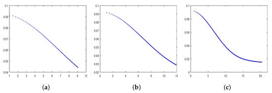
Figure 1. (a) For e = 0.9, the trend in error $\parallel {\tilde{x}}_{n,l}^{\delta }-x^{†}{\parallel }_{H^1[0,1]}$; (b) for e = 0.5, the trend in error $\parallel {\tilde{x}}_{n,l}^{\delta }-x^{†}{\parallel }_{H^1[0,1]}$; (c) for e = 0.1, the trend of error $\parallel {\tilde{x}}_{n,l}^{\delta }-x^{†}{\parallel }_{H^1[0,1]}$. The horizontal axis is $\sqrt{l}$, the vertical axis is $\parallel {\tilde{x}}_{n,l}^{\delta }-x^{†}{\parallel }_{H^1[0,1]}$.

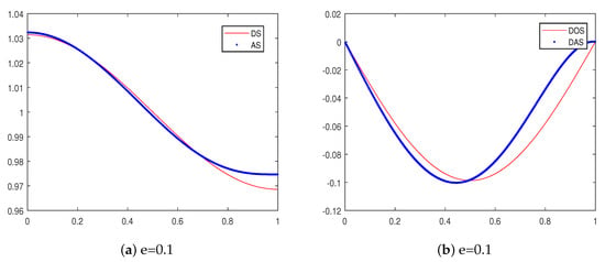
Figure 2. (a) For e = 0.1, the approximate solutions ${\tilde{x}}_{n,l_{*}}^{\delta }$(AS) and $x_0$-minimum-norm solution ${\tilde{x}}^{†}$(OS); (b) for e = 0.1, the generalized derivatives of ${\tilde{x}}_{n,l_{*}}^{\delta }$ (DAS) and $x^{†}$ (DOS).

References

- Scherzer, O.; Grasmair, M.; Grossauer, H.; Haltmeier, M.; Lenzen, F. Variational Methods in Imaging; Springer: New York, NY, USA, 2009; p. 297. [Google Scholar]
- Schuster, T.; Kaltenbacher, B.; Hofmann, B.; Kazimierski, K.S. Regularization Methods in Banach Spaces; Walter de Gruyter: Berlin, Germany, 2012; p. 323. [Google Scholar]
- Engl, H.W.; Neubauer, A.; Scherzer, O. Regularization of Inverse Problems; Kluwer Academic Publishers: Dordrecht, The Netherlands, 1996; p. 329. [Google Scholar]
- Kaltenbacher, B.; Hanke, M.; Neubauer, A. Iterative Regularization Methods for Nonlinear Ill-Posed Problems. Walter de Gruyter: Berlin, Germany; New York, NY, USA, 2008; p. 200. [Google Scholar]
- Jin, Q. On a regularized Levenberg-Marquardt method for solving nonlinear inverse problems. Numer. Math. 2010, 115, 229–259. [Google Scholar] [CrossRef]
- Hochbruck, M.; Honig, M.; Ostermann, A. A convergence analysis of the exponential Euler iteration for nonlinear ill-posed problems. Inverse Probl. 2009, 25, 075009. [Google Scholar] [CrossRef][Green Version]
- Hanke, M. The regularizing Levenberg-Marquardt scheme of optimal order. J. Integral Equ. Appl. 2010, 2, 259–283. [Google Scholar] [CrossRef]
- Ito, K.; Jin, B. Inverse Problems: Tikhonov Theory and Algorithms; World Scientific Publishing Co. Pte. Ltd.: Hackensack, NJ, USA, 2015; p. 330. [Google Scholar]
- Engl, H.W.; Kunisch, K.; Neubauer, A. Convergence rates of Tikhonov regularization of nonlinear ill-posed problems. Inverse Probl. 1989, 5, 523–540. [Google Scholar] [CrossRef]
- Jin, Q. Applications of the modified discrepancy principle to Tikhonov regularization of nonlinear ill-posed problems. SIAM J. Numer. Anal. 1999, 36, 475–490. [Google Scholar]
- Hou, Z.; Jin, Q. Tikhonov regularization for nonlinear ill-posed problems. Nonlinear Anal. 1997, 28, 1799–1809. [Google Scholar] [CrossRef]
- Scherzer, O.; Engl, H.W.; Kunisch, K. Optimal a-posteriori parameter choice for Tikhonov regularization for solving nonlinear ill-posed problems. SIAM J. Numer. Anal. 1993, 30, 1796–1838. [Google Scholar] [CrossRef]
- Jin, Q.; Hou, Z. On an a posteriori parameter choice strategy for Tikhonov regularization of nonlinear ill-posed problems. Numer. Math. 1999, 83, 139–159. [Google Scholar] [CrossRef]
- Hanke, M.; Neubauer, A.; Scherzer, O. A convergence analysis of the Landweber iteration for nonlinear ill-posed problems. Numer. Math. 1995, 72, 21–37. [Google Scholar] [CrossRef]
- Hanke, M. A note on the nonlinear Landweber iteration. Numer. Funct. Anal. Optim. 2014, 35, 1500–1510. [Google Scholar] [CrossRef]
- Jin, Q.; Amato, U. A Discrete Scheme of Landweber Iteration for Solving Nonlinear Ill-Posed Problems. J. Math. Anal. Appl. 2001, 253, 187–203. [Google Scholar] [CrossRef]
- Neubauer, A. Some generalizations for Landweber iteration for nonlinear ill-posed problems in Hilbert scales. J. Inv. Ill-Posed Probl. 2016, 24, 393–406. [Google Scholar] [CrossRef]
- Neubauer, A. A new gradient method for ill-posed problems. Numer. Funct. Anal. Optim. 2017, 39. [Google Scholar] [CrossRef]
- Scherzer, O. A iterative multi-level algorithm for solving nonlinear ill-posed problems. Numer. Math. 1998, 80, 579–600. [Google Scholar] [CrossRef]
- Chen, Z.; Micchelli, C.A.; Xu, Y. Multiscale Methods for Fredholm Integral Equations; Cambridge University Press: Cambridge, UK, 2015; p. 552. [Google Scholar]
- Dicken, V.; Maass, P. Wavelet-Galerkin methods for ill-posed problems. J. Inverse Ill-Posed Probl. 1996, 4, 203–221. [Google Scholar] [CrossRef]
- Chen, Z.; Cheng, S.; Nelakanti, G.; Yang, H. A fast multiscale Galerkin method for the first kind ill-posed integral equations via Tikhonov regularization. Int. J. Comput. Math. 2010, 87, 565–582. [Google Scholar] [CrossRef]
- Fang, W.; Wang, Y.; Xu, Y. An implementation of fast wavelet Galerkin methods for integral equations of the second kind. J. Sci. Comput. 2004, 20, 277–302. [Google Scholar] [CrossRef]
- Luo, X.; Li, F.; Yang, S. A posteriori parameter choice strategy for fast multiscale methods solving ill-posed integral equations. Adv. Comput. Math. 2012, 36, 299–314. [Google Scholar] [CrossRef]
- Chen, Z.; Wu, B.; Xu, Y. Multilevel Augmentation Methods for Differential Equations. Adv. Comput. Math. 2006, 24, 213–238. [Google Scholar] [CrossRef]
- Thongchuay, W.; Puntip, T.; Maleewong, M. Multilevel augmentation method with wavelet bases for singularly perturbed problem. J. Math. Chem. 2013, 51, 2328–2339. [Google Scholar] [CrossRef]
© 2020 by the authors. Licensee MDPI, Basel, Switzerland. This article is an open access article distributed under the terms and conditions of the Creative Commons Attribution (CC BY) license (http://creativecommons.org/licenses/by/4.0/).