Determining Weights in Multi-Criteria Decision Making Based on Negation of Probability Distribution under Uncertain Environment

Abstract

Multi-criteria decision making (MCDM) refers to the decision making in the limited or infinite set of conflicting schemes. At present, the general method is to obtain the weight coefficients of each scheme based on different criteria through the expert questionnaire survey, and then use the Dempster–Shafer Evidence Theory (D-S theory) to model all schemes into a complete identification framework to generate the corresponding basic probability assignment (BPA). The scheme with the highest belief value is then chosen. In the above process, using different methods to determine the weight coefficient will have different effects on the final selection of alternatives. To reduce the uncertainty caused by subjectively determining the weight coefficients of different criteria and further improve the level of multi-criteria decision-making, this paper combines negation of probability distribution with evidence theory and proposes a weights-determining method in MCDM based on negation of probability distribution. Through the quantitative evaluation of the fuzzy degree of the criterion, the uncertainty caused by human subjective factors is reduced, and the subjective error is corrected to a certain extent.

1. Introduction

Multi-criteria decision making (MCDM) refers to the decision making in the limited or infinite set of conflicting schemes. According to whether the alternatives are limited or infinite, MCDM can be divided into multi-attribute decision making (limited) and multi-objective decision making (infinite). In essence, multi-attribute decision-making is mainly used to study the evaluation and optimization of known schemes, and multi-objective decision-making is mainly used to study the planning and design of unknown schemes. This paper mainly discusses the multi-attribute decision-making problem with multiple conflicting attributes. According to the performance of each scheme under different criteria, it carries out a comprehensive evaluation, and then selects the best scheme from the limited schemes. Most of the project decision-making problems in our life can be modeled as multi-criteria decision making problems [1,2,3,4,5]. Because of its universality and importance, the exploration of such problems has shown progress. Many math tools are presented to deal with multi-criteria decision-making, such as fuzzy sets [6,7,8,9,10,11], which offer a framework to address uncertainty and vagueness; soft sets [12,13,14]; evidence theory [15,16,17,18,19], which enables any union of classes to be addressed and expresses both uncertainty and imprecision; Z numbers [20], which can not only express uncertainty, imprecision and incompleteness of information but can also represent the reliability of information; D numbers [21,22], which are more capable of expressing and handling both uncertainty and imprecision; network modeling [23,24,25]; etc. [26].

In the process of solving multi-criteria decision making problems, the determination of criteria weight is very important. It is used to reflect the relative importance of a certain criterion. If a certain criterion is relatively important, it is given a relatively large weight; otherwise, it is given a relatively small weight. There are three methods to determine the weight: subjective method, objective method, and comprehensive method. At present, the general solution is the comprehensive method. First, the alternatives are subjectively evaluated by experts based on various criteria. Then, the linguistic evaluation is converted to the corresponding quantitative evaluation; a comprehensive measure of subjective evaluation and objective reflection is calculated through certain rules; and finally the alternatives are evaluated, ranked and optimized [27,28]. On this basis, Fei et al. developed a MCDM method where the evaluation information is expressed and handled by Dempster–Shafer theory [29]. In the evaluation of a scheme, the evaluation under each criterion affects the final result to some extent [30,31,32]. Due to the relative importance difference between different criteria, the final evaluation results are obtained by evaluating the importance degree of each criterion and weighting the evaluation based on each criterion, respectively. The relatively important criterion has a larger weight, and the corresponding evaluation of the criterion has a greater impact on the final results. On the contrary, the relatively unimportant criterion has a smaller weight, and the corresponding evaluation of the criterion has a smaller impact on the final result. Thus, we need to assign an appropriate weight to each influencing factor carefully to reduce the impact of subjective factors on the result. To solve this problem, we carefully studied some methods to determine the combination weight, such as the method for obtaining ordered weighted average OWA weights proposed by Xu, which can relieve the influence of unfair arguments on the decision results [33]; the method to obtain a weights vector [34] proposed by Lamata et al.; the PPMIS (Project and Portfolio Management Information Systems) selection/evaluation approach that combines TOPSIS (Technique for Order Preference by Similarity to Ideal Solution) with intuitionistic fuzzy group decision making presented by Gerogiannis et al. [35]; and two reliability-based combination rules are used to synthesize multi-source information [36].

Furthermore, to improve the level of decision-making in uncertain environment, researchers have previously carried out long-term and in-depth studiesy. Srivastava et al. defined a new entropy function for determination of uncertainty associated with the negation of a probability distribution and the events associated with it [37]. Srivastava et al. also developed uncertainty measures that measure the uncertainty associated with the negation of a probability distribution [38]. Luo and Deng presented a new definition of negation of BBA [39], which is used to measure fuzziness for D-S theory. Xie and Xiao proposed negation method of BPA based on the maximum uncertainty [40]. The negation of probability distribution provides a new view to represent the uncertainty information, which leads to the application of negation of probability distribution in related fields and in-depth exploration [41]. In addition, the negation model has the maximum entropy allocation, which attracts studies on uncertainty measures that can be applied in the negation process.

Recently, Xiao proposed a method of evidence fuzzy multi-criteria decision-making based on belief entropy, named as EFMCDM [42]. The combination of D-S evidence theory and belief entropy should be used to solve the problem of multi-criteria decision making. First, the experts evaluate the linguistic rating of all alternatives and the importance of each criterion based on each criterion. Then, the fuzzy number is used to transform the language level evaluation into quantitative evaluation of numbers, and then the weighted decision matrix is obtained through a series of calculations. Then, the D-S evidence theory is used to model the whole scheme into a complete identification framework, and the BPA of each criterion is generated by using the belief entropy. After fusing multiple pieces of evidence, the best scheme is selected according to the belief value of the alternatives. In the process of decision-making, EFMCDM considers the influence of subjective and objective weight, and builds a quantitative model of uncertainty, which successfully reduces the uncertainty brought by human subjective cognition and improves the decision-making level.

However, EFMCDM does not consider the fuzziness of evaluation criteria. To further improve the decision-making level, this paper proposes a weights-determining method in MCDM based on negation of probability distribution [43] under uncertain environment. In the process of constructing the weighted decision matrix, it can be found that the column elements in the final weighted decision matrix satisfy the probability distribution. The probability distribution of each criterion has its corresponding negation, thus the distance between the probability distributions and its negation can be used to measure the fuzzy degree of the corresponding criterion. Specifically, this paper mainly deals with the weight determination method of the multi-attribute decision-making problem, aiming at the optimization problem of limited schemes, using the negation of (discrete) probability distribution to propose feasible solutions. As defined in the original paper [43], the negation of a (discrete) probability distribution is based on the sample size and closely related to the sample probability measure. Because the number of schemes and criteria is limited, and the weights of different schemes with the same criteria meet the definition of discrete distribution after normalization, the negation of probability distribution can be applied to the weight determination of multi-attribute decision making.

Here is an example to understand the above ideas. Two sets of propositions are considered: proposition “he may be a good man” and its negative proposition “he may not be a good man”, and proposition “he is absolutely a good man” and its negative proposition “he is absolutely not a good man”. Compared with the second group, the two propositions in the first group can obviously feel their distance is closer, and this group of propositions is also more fuzzy. Therefore, the fuzzy degree of a proposition can be measured by the distance between a proposition and its negation. The higher is the fuzzy degree of a criterion, the greater is the uncertainty of the criterion, and the smaller is the corresponding discount coefficient; conversely, the lower is the fuzzy degree of a criterion, the smaller is the uncertainty of the criterion, and the larger is the corresponding discount coefficient. Based on the negation of probability distribution, the fuzzy degree of the criterion is taken as the reference standard to calculate the discount coefficient of the criterion, and then the BPA of the criterion is generated and combined. In this way, the errors caused by the experts’ subjective evaluation of each standard are corrected and the decision-making level is improved.

The main aim of this study is to provide a new way to solve the multi criteria decision-making problem by combining the negation of probability distribution and evidence fusion from the point of quantitative description of the fuzzy degree of criteria.

2. Preliminaries

2.1. Dempster–Shafer Evidence Theory

How to handle the problem of uncertainty has received much attention in recent years [44,45]. Thus far, various methods have been exploited, including grey prediction model [46], network model [47,48], risk-based model [49,50,51,52], evidential reasoning [53,54], entropy-based [55,56,57], etc. These methods were used in many applications, e.g. failure analysis [58,59], risk assessments [60], reliability evaluation [61,62], classification [63,64], and decision-making [65,66,67,68]. As one of the most effective methods, D-S evidence theory [69,70] is a kind of imprecise reasoning theory, which satisfies the axiomatic system weaker than probability theory. The main knowledge we need to master includes: the basic concepts of D-S evidence theory (identification framework, proposition, and basic probability distribution), and combination rules.

Theorem 1.

The identification framework Θ is defined as an exhaustive set of all possible values that are mutually exclusive to variables [69,70].

$$\mathsf{\Theta }=\{A_1,A_2,\cdots ,A_n\}$$

(1)

Theorem 2.

The power set $2^{\mathsf{\Theta }}$ is defined as the set of all combinations of possible cases in the identification framework, that is, the set of all subsets of the identification framework Θ. Proposition A is a subset of the identification framework Θ, that is, the elements of the power set $2^{\mathsf{\Theta }}$ [69,70].

$$2^{\mathsf{\Theta }}=\{\varnothing ,\left\{A_1\right\},\cdots ,\left\{A_n\right\},\{A_1,A_2\},\cdots ,\{A_1,A_2,\cdots ,A_i\},\cdots ,\mathsf{\Theta }\}$$

(2)

Theorem 3.

BPA is the basic probability distribution function and m meets the following two conditions: $m(\varnothing )=0$ and ${\displaystyle \sum _{A\subseteq \mathsf{\Theta }}}m\left(A\right)=1$. $m\left(A\right)$ represents the precise trust degree to proposition A, which means that you do not know how to allocate this number when $A=\mathsf{\Omega }$ [69,70].

Since BPA is effective to model the uncertain information, it has been well studied, e.g. for divergence measure [71,72], distance measure [73], correlation coefficient [74,75], entropy measure [76,77,78], dependent evidence [79], etc. [80,81].

Theorem 4.

The combination rule is to calculate the orthogonal sum of different probability distribution functions [69,70].

$$m\left(A\right)=m_1\oplus m_2=\left\{\begin{array}{c}0,A=\varphi \hfill \\ \frac{{\sum }_{A_1\cap A_2=A}{m}_1\left(A_1\right)m_2\left(A_2\right)}{1-{\sum }_{A_1\cap A_2=\varphi }{m}_1\left(A_1\right)m_2\left(A_2\right)}\hfill \end{array},A\ne \varphi \right.$$

(3)

2.2. Negation of Probability Distribution

The negation of probability distribution [43] generally does not lead to the unique probability distribution, but generates a set of probability distributions that is regarded as consistent with the negation idea. Specially, based on the maximum entropy distribution of the weight related to each focus element, there is a unique negative implementation.

Theorem 5.

Probability distribution. If the reference system is set $X=\{x_1,x_2,\cdots ,x_n\}$ and $P=\{p_1,p_2,\cdots ,p_n\}$ is the probability distribution of X, the following requirements should be met [43]:

$$\left\{\begin{array}{c}\sum p_i=1\hfill \\ p_i\in [0,1]\hfill \end{array}\right.$$

(4)

Theorem 6.

Negation of probability distribution. $\overline{P}=\{\overline{p_1},\overline{p_2},\cdots ,\overline{p_n}\}$ is the negation of probability distribution P [43],

$$\overline{p_i}=\frac{1-p_i}{n-1}$$

(5)

Because ${\sum }_{i=1}^n\overline{p_i}=\frac{1}{n-1}{\sum }_{i=1}^n\left(1-p_i\right)=1$ and $\overline{p_i}\in [0,1]$, $\overline{P}$ is also a probability distribution.

3. Proposed Method

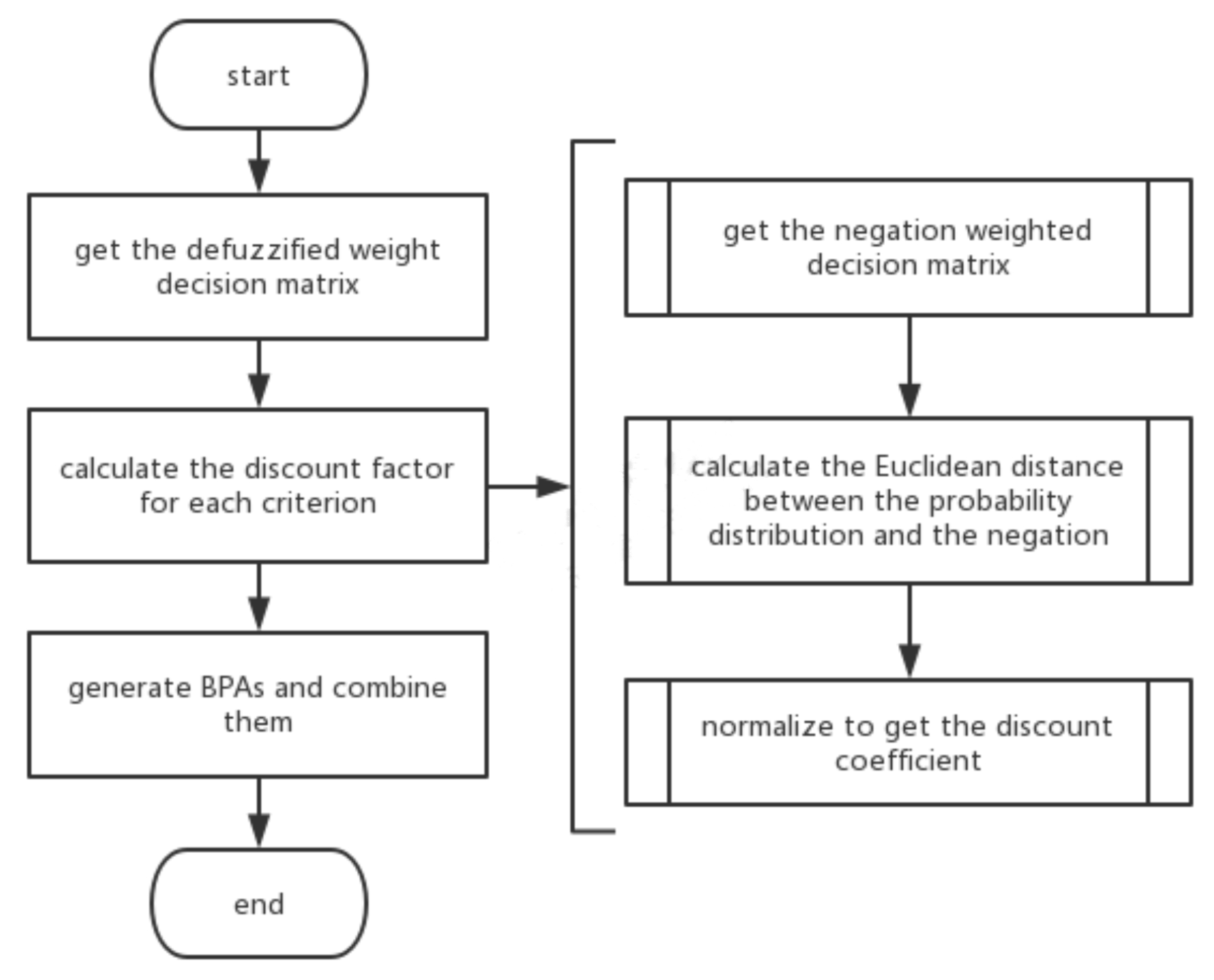
In this section, we introduce a multi-criteria decision-making method based on negation of probability distribution. The specific flow chart is shown in Figure 1. By combining the D-S evidence theory with the negation of probability distribution, the fuzzy degree of the criterion is taken as the reference standard to calculate the discount coefficient of the criterion, which corrects the errors brought by the experts’ subjective evaluation of each criterion and improves the decision making level.

Problem statement: Let a set of m possible exclusive alternatives $\mathsf{\Theta }=\{A_1,A_2,\cdots ,A_m\}$ be the frame of discernment, $C=\{C_1,C_2,\cdots ,C_n\}$ be the set of n decision criteria, and $DM=\{D{M}_1,D{M}_2,\cdots ,D{M}_t\}$ be the set of t decision makers. A set of fuzzy ratings for $A_i(i=1,2,\cdots ,m)$ with respect to the criteria $C_j(j=1,2,\cdots ,n)$ given by the decision maker $D{M}_k(k=1,2,\cdots ,t)$ is denoted as $\widetilde{x_{ijk}},i=1,2,\cdots ,m;j=1,2,\cdots ,n;k=1,2,\cdots ,t$, where $\widetilde{x_{ijk}}=(x_{ijk1},x_{ijk2},x_{ijk3},x_{ijk4})$, and a set of fuzzy importance weights for $C_j(j=1,2,\cdots ,n)$ given by the decision maker $D{M}_k(k=1,2,\cdots ,t)$ is denoted as $\widetilde{w_{jk}},j=1,2,\cdots ,n;k=1,2,\cdots ,t$, where $\widetilde{w_{jk}}=(w_{jk1},w_{jk2},w_{jk3},w_{jk4})$. Consider this fuzzy MCDM problem: The best candidate should be selected from $\theta$.

Step 1: According to Xiao’s idea [42], obtain the normalized defuzzified weight decision matrix $\overline{D}ef\left(\overline{\tilde{D}}\right)$.

Step 1-1: Multiply fuzzy coefficient $\widetilde{x_{ijk}}$ and fuzzy importance weight $\widetilde{w_{jk}}$ to get weighted fuzzy coefficient ${\tilde{x}}_{ijk}^w={\tilde{x}}_{ijk}\times {\tilde{w}}_{jk}$, where the superscript w is used to represent the weight of importance of different criteria. Due to different decision makers having different judgments on the importance degree of different criteria, by scalar multiplication, the weight factors ($\widetilde{x_{ijk}}$) of the same criteria of the same decision-maker and the importance factors ($\widetilde{w_{jk}}$) of the criteria are multiplied correspondingly, and the weighted weight factors (${\tilde{x}}_{ijk}^w$) of a decision-maker for a scheme under a certain criterion are obtained. Then, the weighted fuzzy coefficient matrix ${\tilde{D}}_k(k=1,2,\dots ,t)$ is obtained:

$${\tilde{D}}_k=\left[\begin{array}{ccccc}{\tilde{x}}_{11k}^w& \cdots & {\tilde{x}}_{1jk}^w& \cdots & {\tilde{x}}_{ink}^w\\ ⋮& ⋮& ⋮& ⋮& ⋮\\ {\tilde{x}}_{i1k}^w& \cdots & {\tilde{x}}_{ijk}^w& \cdots & {\tilde{x}}_{ink}^w\\ ⋮& ⋮& ⋮& ⋮& ⋮\\ {\tilde{x}}_{m1k}^w& \cdots & {\tilde{x}}_{mjk}^w& \cdots & {\tilde{x}}_{mnk}^w\end{array}\right]$$

(6)

Step 1-2: The aggregated fuzzy value ${\tilde{x}}_{ij}^w$ of weighted fuzzy value and the aggregated decision matrix $\tilde{D}$ are obtained by considering the evaluation of t decision-makers. Then, the aggregated fuzzy values are normalized and defuzzified, respectively. Then, the defuzzified weight decision matrix $Def\left(\overline{\tilde{D}}\right)$ is obtained. After another normalization, obtain $\overline{D}ef\left({\overline{\tilde{x}}}_{ij}^w\right)=\frac{Def\left({\overline{\tilde{x}}}_{ij}^w\right)}{{\sum }_{s=1}^{m}Def\left({\overline{\tilde{x}}}_{sj}^w\right)},j=1,2,\dots ,n$. Then, the normalized defuzzified weight decision matrix is obtained:

$$\overline{D}ef\left(\overline{\tilde{D}}\right)=\left[\begin{array}{ccccc}\overline{D}ef\left({\overline{\tilde{x}}}_{11}^w\right)& \cdots & \overline{D}ef\left({\overline{\tilde{x}}}_{1j}^w\right)& \cdots & \overline{D}ef\left({\overline{\tilde{x}}}_{1n}^w\right)\\ ⋮& ⋮& ⋮& ⋮& ⋮\\ \overline{D}ef\left({\overline{\tilde{x}}}_{i1}^w\right)& \cdots & \overline{D}ef\left({\overline{\tilde{x}}}_{ij}^w\right)& \cdots & \overline{D}ef\left({\overline{\tilde{x}}}_{in}^w\right)\\ ⋮& ⋮& ⋮& ⋮& ⋮\\ \overline{D}ef\left({\overline{\tilde{x}}}_{m1}^w\right)& \cdots & \overline{D}ef\left({\overline{\tilde{x}}}_{mj}^w\right)& \cdots & \overline{D}ef\left({\overline{\tilde{x}}}_{mn}^w\right)\end{array}\right]$$

(7)

Step 2: Calculate the discount factor for each criterion.

Step 2-1: Since the column elements of the above matrix are obtained by normalization, $\overline{D}ef\left({\overline{\tilde{x}}}_{ij}^w\right)=\frac{Def\left({\overline{\tilde{x}}}_{ij}^w\right)}{{\sum }_{s=1}^{m}Def\left({\overline{\tilde{x}}}_{sj}^w\right)},j=1,2,\dots n$, each column conforms to the characteristics of probability distribution. Through the negation formula,

$$N\overline{D}ef\left({\overline{\tilde{x}}}_{ij}^w\right)=\frac{1-\overline{D}ef\left({\overline{\tilde{x}}}_{ij}^w\right)}{m-1}$$

(8)

the negation weighted decision matrix $N\overline{D}ef\left(\overline{\tilde{D}}\right)$ can be obtained.

$$N\overline{D}ef\left(\overline{\tilde{D}}\right)=\left[\begin{array}{ccccc}N\overline{D}ef\left({\overline{\tilde{x}}}_{11}^w\right)& \cdots & N\overline{D}ef\left({\overline{\tilde{x}}}_{1j}^w\right)& \cdots & N\overline{D}ef\left({\overline{\tilde{x}}}_{1n}^w\right)\\ ⋮& ⋮& ⋮& ⋮& ⋮\\ N\overline{D}ef\left({\overline{\tilde{x}}}_{i1}^w\right)& \cdots & N\overline{D}ef\left({\overline{\tilde{x}}}_{ij}^w\right)& \cdots & N\overline{D}ef\left({\overline{\tilde{x}}}_{in}^w\right)\\ ⋮& ⋮& ⋮& ⋮& ⋮\\ N\overline{D}ef\left({\overline{\tilde{x}}}_{m1}^w\right)& \cdots & N\overline{D}ef\left({\overline{\tilde{x}}}_{mj}^w\right)& \cdots & N\overline{D}ef\left({\overline{\tilde{x}}}_{mn}^w\right)\end{array}\right]$$

(9)

Step 2-2: For each criterion $C_j$, the Euclidean distance $d_j$ between the probability distribution and the negation is calculated.

$$d_j=\sqrt{\sum _{i=1}^m{\left[\overline{D}ef\left({\overline{\tilde{x}}}_{ij}^w\right)-N\overline{D}ef\left({\overline{\tilde{x}}}_{ij}^w\right)\right]}^2},j=1,2,\dots ,n$$

(10)

Step 2-3: Normalize to get the discount coefficient $U_{C_j}$ of each criterion.

$$U_{C_j}=\frac{d_j}{{\sum }_{j=1}^n{d}_j},j=1,2,\dots ,n$$

(11)

Step 3: Generate BPAs and combine them.

Step 3-1: According to the following formula, BPA corresponding to each proposition $A_i$ is generated based on each criterion $C_j$.

$$\left\{\begin{array}{c}{m}_{C_j}\left(\varphi \right)=0\hfill \\ m_{C_j}\left(A_i\right)=\overline{D}ef\left({\overline{\tilde{x}}}_{ij}^w\right)\times U_{C_j},i=1,2,\dots ,m,j=1,2,\dots ,n\hfill \\ m_{C_j}\left(\mathsf{\Theta }\right)=1-\sum _{i=1}^m{m}_{C_j}\left(A_i\right)\hfill \end{array}\right.$$

(12)

Step 3-2: Through (n−1) times orthogonal sum operation, BPAs of different criteria are combined with each other.

$$m_C=\left(\cdots \left(m_{C_1}\oplus m_{C_2}\right)\oplus \cdots \oplus m_{C_n}\right)$$

(13)

Step 3-3: According to the value of $m_C$, the scheme $A_{\alpha }$ with the largest $m_C$ is the best scheme, and the best scheme may not be unique.

$$\alpha =\underset{1\le i\le m}{argmax}\left\{m_C\right\}$$

(14)

4. Examples

In this section, the feasibility of the proposed method is verified by experiments.

4.1. Problem Statement

Problem statement: Consider the decision-making problem of supplier selection from Xiao [42] associated with a committee of three decision makers established by a company who give their anticipation and definition of the evaluation criteria for the final four candidate suppliers after a preliminary screening, where $\mathsf{\Theta }=\{A_1,A_2,A_3,A_4\}$ is the frame of discernment consisting of four alternatives, $DM=\{D{M}_1,D{M}_2,D{M}_3\}$ is the set of decision makers, and $C=\{C_1,C_2,C_3,C_4,C_5\}$ is the set of criteria, which is considered to be the set of evidence. The criteria are defined as follows: C1 is the quality of products, C2 is the effort to establish cooperation, C3 is the technical level of each supplier, C4 is the delay on delivery of each supplier, and C5 is the price/cost.

A set of fuzzy ratings $\widetilde{x_{ijk}},i=1,2,3,4;j=1,2,3,4,5;k=1,2,3$ for $A_i(i=1,2,3,4)$ with respect to the criteria $C_j(j=1,2,3,4,5)$ given by the decision maker $D{M}_k(k=1,2,3)$ is shown in

Table 1. A set of fuzzy ratings ${\tilde{X}}_k$.

$\mathit{D}1$	${\mathit{C}}_1$	${\mathit{C}}_2$	${\mathit{C}}_3$	${\mathit{C}}_4$	${\mathit{C}}_5$
$A_1$	(0.5, 0.6, 0.7, 0.8)	(0.4, 0.5, 0.5, 0.6)	(0.5, 0.6, 0.7, 0.8)	(0.7, 0.8, 0.8, 0.9)	(0.8, 0.9, 1.0, 1.0)
$A_2$	(0.5, 0.6, 0.7, 0.8)	(0.5, 0.6, 0.7, 0.8)	(0.7, 0.8, 0.8, 0.9)	(0.7, 0.8, 0.8, 0.9)	(0.5, 0.6, 0.7, 0.8)
$A_3$	(0.7, 0.8, 0.8, 0.9)	(0.5, 0.6, 0.7, 0.8)	(0.4, 0.5, 0.5, 0.6)	(0.5, 0.6, 0.7, 0.8)	(0.8, 0.9, 1.0, 1.0)
$A_4$	(0.8, 0.9, 1.0, 1.0)	(0.7, 0.8, 0.8, 0.9)	(0.7, 0.8, 0.8, 0.9)	(0.5, 0.6, 0.7, 0.8)	(0.7, 0.8, 0.8, 0.9)
$\mathit{D}\mathbf{2}$	${\mathit{C}}_{\mathbf{1}}$	${\mathit{C}}_{\mathbf{2}}$	${\mathit{C}}_{\mathbf{3}}$	${\mathit{C}}_{\mathbf{4}}$	${\mathit{C}}_{\mathbf{5}}$
$A_1$	(0.7, 0.8, 0.8, 0.9)	(0.5, 0.6, 0.7, 0.8)	(0.7, 0.8, 0.8, 0.9)	(0.7, 0.8, 0.8, 0.9)	(0.8, 0.9, 1.0, 1.0)
$A_2$	(0.5, 0.6, 0.7, 0.8)	(0.5, 0.6, 0.7, 0.8)	(0.5, 0.6, 0.7, 0.8)	(0.5, 0.6, 0.7, 0.8)	(0.5, 0.6, 0.7, 0.8)
$A_3$	(0.8, 0.9, 1.0, 1.0)	(0.7, 0.8, 0.8, 0.9)	(0.4, 0.5, 0.5, 0.6)	(0.5, 0.6, 0.7, 0.8)	(0.8, 0.9, 1.0, 1.0)
$A_4$	(0.7, 0.8, 0.8, 0.9)	(0.5, 0.6, 0.7, 0.8)	(0.8, 0.9, 1.0, 1.0)	(0.7, 0.8, 0.8, 0.9)	(0.7, 0.8, 0.8, 0.9)
$\mathit{D}\mathbf{3}$	${\mathit{C}}_{\mathbf{1}}$	${\mathit{C}}_{\mathbf{2}}$	${\mathit{C}}_{\mathbf{3}}$	${\mathit{C}}_{\mathbf{4}}$	${\mathit{C}}_{\mathbf{5}}$
$A_1$	(0.5, 0.6, 0.7, 0.8)	(0.8, 0.9, 1.0, 1.0)	(0.7, 0.8, 0.8, 0.9)	(0.5, 0.6, 0.7, 0.8)	(0.5, 0.6, 0.7, 0.8)
$A_2$	(0.5, 0.6, 0.7, 0.8)	(0.7, 0.8, 0.8, 0.9)	(0.7, 0.8, 0.8, 0.9)	(0.7, 0.8, 0.8, 0.9)	(0.7, 0.8, 0.8, 0.9)
$A_3$	(0.7, 0.8, 0.8, 0.9)	(0.5, 0.6, 0.7, 0.8)	(0.5, 0.6, 0.7, 0.8)	(0.5, 0.6, 0.7, 0.8)	(0.7, 0.8, 0.8, 0.9)
$A_4$	(0.7, 0.8, 0.8, 0.9)	(0.5, 0.6, 0.7, 0.8)	(0.8, 0.9, 1.0, 1.0)	(0.5, 0.6, 0.7, 0.8)	(0.5, 0.6, 0.7, 0.8)

, and a set of fuzzy importance weights $\widetilde{w_{jk}},j=1,2,3,4,5;k=1,2,3$ for $C_j(j=1,2,3,4,5)$ given by the decision maker $D{M}_k(k=1,2,3)$ is shown in

Table 2. A set of fuzzy importance weights ${\tilde{W}}_k$.

$\widetilde{{\mathit{w}}_{\mathit{jk}}}$	${\mathit{C}}_1$	${\mathit{C}}_2$	${\mathit{C}}_3$	${\mathit{C}}_4$	${\mathit{C}}_5$
$D_1$	(0.2, 0.3, 0.4, 0.5)	(0.4, 0.5, 0.5, 0.6)	(0.7, 0.8, 0.8, 0.9)	(0.8, 0.9, 1.0, 1.0)	(0.7, 0.8, 0.8, 0.9)
$D_2$	(0.2, 0.3, 0.4, 0.5)	(0.2, 0.3, 0.4, 0.5)	(0.8, 0.9, 1.0, 1.0)	(0.8, 0.9, 1.0, 1.0)	(0.5, 0.6, 0.7, 0.8)
$D_3$	(0.4, 0.5, 0.5, 0.6)	(0.4, 0.5, 0.5, 0.6)	(0.8, 0.9, 1.0, 1.0)	(0.8, 0.9, 1.0, 1.0)	(0.5, 0.6, 0.7, 0.8)

.

4.2. Implementation Based on the Proposed Method

Step 1: Get the normalized defuzzified weight decision matrix.

Step 1-1: Generate the fuzzy values of the weighted supplier ratings ${\tilde{x}}_{ijk}^w$. Then, the weighted fuzzy coefficient matrix ${\tilde{D}}_k$ is obtained, as shown in

Table 3. The weighted fuzzy coefficient matrix ${\tilde{D}}_k$.

$\mathit{D}1$	${\mathit{C}}_1$	${\mathit{C}}_2$	${\mathit{C}}_3$	${\mathit{C}}_4$	${\mathit{C}}_5$
$A_1$	(0.10, 0.18, 0.28, 0.40)	(0.16, 0.27, 0.40, 0.50)	(0.35, 0.48, 0.56, 0.72)	(0.56, 0.72, 0.80, 0.90)	(0.56, 0.72, 0.80, 0.90)
$A_2$	(0.10, 0.18, 0.28, 0.40)	(0.20, 0.30, 0.35, 0.48)	(0.49, 0.64, 0.64, 0.81)	(0.56, 0.72, 0.80, 0.90)	(0.35, 0.48, 0.56, 0.72)
$A_3$	(0.14, 0.24, 0.32, 0.45)	(0.20, 0.30, 0.35, 0.48)	(0.28, 0.40, 0.40, 0.54)	(0.40, 0.54, 0.70, 0.80)	(0.56, 0.72, 0.80, 0.90)
$A_4$	(0.16, 0.27, 0.40, 0.50)	(0.28, 0.40, 0.40, 0.54)	(0.49, 0.64, 0.64, 0.81)	(0.40, 0.54, 0.70, 0.80)	(0.49, 0.64, 0.64, 0.81)
$\mathit{D}\mathbf{2}$	${\mathit{C}}_{\mathbf{1}}$	${\mathit{C}}_{\mathbf{2}}$	${\mathit{C}}_{\mathbf{3}}$	${\mathit{C}}_{\mathbf{4}}$	${\mathit{C}}_{\mathbf{5}}$
$A_1$	(0.14, 0.24, 0.32, 0.45)	(0.10, 0.18, 0.28, 0.40)	(0.56, 0.72, 0.80, 0.90)	(0.56, 0.72, 0.80, 0.90)	(0.40, 0.54, 0.70, 0.80)
$A_2$	(0.10, 0.18, 0.28, 0.40)	(0.10, 0.18, 0.28, 0.40)	(0.40, 0.54, 0.70, 0.80)	(0.40, 0.54, 0.70, 0.80)	(0.25, 0.36, 0.49, 0.64)
$A_3$	(0.16, 0.27, 0.40, 0.50)	(0.14, 0.24, 0.32, 0.45)	(0.32, 0.45, 0.50, 0.60)	(0.40, 0.54, 0.70, 0.80)	(0.40, 0.54, 0.70, 0.80)
$A_4$	(0.14, 0.24, 0.32, 0.45)	(0.10, 0.18, 0.28, 0.40)	(0.64, 0.81, 1.00, 1.00)	(0.56, 0.72, 0.80, 0.90)	(0.35, 0.48, 0.56, 0.72)
$\mathit{D}\mathbf{3}$	${\mathit{C}}_{\mathbf{1}}$	${\mathit{C}}_{\mathbf{2}}$	${\mathit{C}}_{\mathbf{3}}$	${\mathit{C}}_{\mathbf{4}}$	${\mathit{C}}_{\mathbf{5}}$
$A_1$	(0.20, 0.30, 0.35, 0.48)	(0.32, 0.45, 0.50, 0.60)	(0.56, 0.72, 0.80, 0.90)	(0.40, 0.54, 0.70, 0.80)	(0.25, 0.36, 0.49, 0.64)
$A_2$	(0.20, 0.30, 0.35, 0.48)	(0.28, 0.40, 0.40, 0.54)	(0.56, 0.72, 0.80, 0.90)	(0.56, 0.72, 0.80, 0.90)	(0.35, 0.48, 0.56, 0.72)
$A_3$	(0.28, 0.40, 0.40, 0.54)	(0.20, 0.30, 0.35, 0.48)	(0.40, 0.54, 0.70, 0.80)	(0.40, 0.54, 0.70, 0.80)	(0.35, 0.48, 0.56, 0.72)
$A_4$	(0.28, 0.40, 0.40, 0.54)	(0.20, 0.30, 0.35, 0.48)	(0.64, 0.81, 1.00, 1.00)	(0.40, 0.54, 0.70, 0.80)	(0.25, 0.36, 0.49, 0.64)

.

Step 1-2: By integrating evaluations from different decision makers, the aggregated fuzzy value of weighted fuzzy value ${\tilde{x}}_{ij}^w$ can be obtained, as shown in

Table 4. The normalized aggregated decision matrix $\tilde{D}$.

${\tilde{\mathit{x}}}_{\mathit{ij}}^{\mathit{w}}$	${\mathit{C}}_1$	${\mathit{C}}_2$	${\mathit{C}}_3$	${\mathit{C}}_4$	${\mathit{C}}_5$
$A_1$	(0.10, 0.24, 0.32, 0.48)	(0.10, 0.29, 0.34, 0.60)	(0.35, 0.64, 0.72, 0.90)	(0.40, 0.66, 0.77, 0.90)	(0.25, 0.54, 0.66, 0.90)
$A_2$	(0.10, 0.22, 0.30, 0.48)	(0.10, 0.29, 0.34, 0.54)	(0.40, 0.63, 0.71, 0.90)	(0.40, 0.66, 0.77, 0.90)	(0.25, 0.44, 0.54, 0.72)
$A_3$	(0.14, 0.30, 0.37, 0.54)	(0.14, 0.28, 0.34, 0.48)	(0.28, 0.46, 0.53, 0.80)	(0.40, 0.54, 0.70, 0.80)	(0.35, 0.58, 0.69, 0.90)
$A_4$	(0.14, 0.30, 0.37, 0.54)	(0.10, 0.29, 0.34, 0.54)	(0.49, 0.75, 0.88, 1.00)	(0.40, 0.66, 0.77, 0.90)	(0.25, 0.49, 0.56, 0.81)

. Through the normalization and the defuzzification, the defuzzified weight decision matrix $Def\left(\overline{\tilde{D}}\right)$ can be obtained, as shown in

Table 5. The defuzzified weight decision matrix $Def\left(\overline{\tilde{D}}\right)$.

$\mathit{Def}\left({\overline{\tilde{\mathit{x}}}}_{\mathit{ij}}^{\mathit{w}}\right)$	${\mathit{C}}_1$	${\mathit{C}}_2$	${\mathit{C}}_3$	${\mathit{C}}_4$	${\mathit{C}}_5$
$A_1$	0.53	3.38	0.65	1.69	2.34
$A_2$	0.52	3.19	0.66	1.69	1.95
$A_3$	0.63	3.10	0.52	1.52	2.51
$A_4$	0.63	3.19	0.77	1.64	2.12

. Then, through another normalization, the normalized defuzzified weight decision matrix $\overline{D}ef\left(\overline{\tilde{D}}\right)$ can be obtained, as shown in

Table 6. The normalized defuzzified weight decision matrix $\overline{D}ef\left(\overline{\tilde{D}}\right)$.

$\overline{\mathit{D}}\mathit{ef}\left({\overline{\tilde{\mathit{x}}}}_{\mathit{ij}}^{\mathit{w}}\right)$	${\mathit{C}}_1$	${\mathit{C}}_2$	${\mathit{C}}_3$	${\mathit{C}}_4$	${\mathit{C}}_5$
$A_1$	0.2296	0.2629	0.2481	0.2581	0.2626
$A_2$	0.2243	0.2481	0.2531	0.2581	0.2181
$A_3$	0.2730	0.2408	0.2015	0.2327	0.2818
$A_4$	0.2730	0.2481	0.2973	0.2511	0.2375

.

Step 2: Calculate the discount factor of each criterion.

Step 2-1: Through the negation formula, the negation weighted decision matrix $N\overline{D}ef\left(\overline{\tilde{D}}\right)$ can be obtained, as shown in

Table 7. The negation weighted decision matrix $N\overline{D}ef\left(\overline{\tilde{D}}\right)$.

$\mathit{N}\overline{\mathit{D}}\mathit{ef}\left({\overline{\tilde{\mathit{x}}}}_{\mathit{ij}}^{\mathit{w}}\right)$	${\mathit{C}}_1$	${\mathit{C}}_2$	${\mathit{C}}_3$	${\mathit{C}}_4$	${\mathit{C}}_5$
$A_1$	0.2568	0.2457	0.2506	0.2473	0.2458
$A_2$	0.2586	0.2506	0.2490	0.2473	0.2606
$A_3$	0.2423	0.2531	0.2662	0.2558	0.2394
$A_4$	0.2423	0.2506	0.2342	0.2496	0.2542

.

Step 2-2: The Euclidean distance $d_j$ of each criterion is calculated by the difference between the weighted decision matrix and its negation matrix, as shown in

Table 8. The difference between the weighted decision matrix and its negation matrix.

Difference Value	${\mathit{C}}_1$	${\mathit{C}}_2$	${\mathit{C}}_3$	${\mathit{C}}_4$	${\mathit{C}}_5$
$A_1$	−0.0272	0.0172	−0.0025	0.0108	0.0168
$A_2$	−0.0343	−0.0025	0.0041	0.0108	−0.0425
$A_3$	0.0307	−0.0123	−0.0647	0.0231	0.0424
$A_4$	0.0307	−0.0025	0.0631	0.0015	−0.0167

and

Table 9. The Euclidean distance $d_j$.

${\mathit{C}}_1$	${\mathit{C}}_2$	${\mathit{C}}_3$	${\mathit{C}}_4$	${\mathit{C}}_5$
0.0617	0.0214	0.0905	0.0277	0.0645

.

Step 2-3: Normalize to get the discount coefficient $U_{C_j}$ of each criterion, as shown in

Table 10. The discount coefficient $U_{C_j}$.

${\mathit{C}}_1$	${\mathit{C}}_2$	${\mathit{C}}_3$	${\mathit{C}}_4$	${\mathit{C}}_5$
0.2319	0.0806	0.3404	0.1043	0.2427

.

Step 3: Generate BPAs and combine them.

Step 3-1: According to the following formula, BPA corresponding to each proposition $A_i$ is generated based on each criterion $C_j$, as shown in

Table 11. The BPAs of the propositions with respect to different criteria.

BPAs	${\mathit{C}}_1$	${\mathit{C}}_2$	${\mathit{C}}_3$	${\mathit{C}}_4$	${\mathit{C}}_5$
$m\left(A_1\right)$	0.0532	0.0212	0.0845	0.0269	0.0637
$m\left(A_2\right)$	0.0520	0.0200	0.0862	0.0269	0.0529
$m\left(A_3\right)$	0.0633	0.0194	0.0686	0.0243	0.0684
$m\left(A_4\right)$	0.0633	0.0200	0.1012	0.0262	0.0577
$m\left(\theta \right)$	0.7681	0.9194	0.6596	0.8957	0.7573

.

Step 3-2: Combine BPAs of different criteria $C_j$ each other, as shown in

Table 12. The combined BPAs of the propositions.

${\mathit{A}}_1$	${\mathit{A}}_2$	${\mathit{A}}_3$	${\mathit{A}}_4$
0.1502	0.1428	0.1456	0.1641

.

Step 3-3: Sort the $m_C$ of different schemes $A_i$ in descending order, and select the best scheme $A_4$.

4.3. Comparison and Discussion

We compare the proposed method with the related methods, i.e., EFMCDM [42], where the experimental results are shown in

Table 13. Comparison of the proposed method with EFMCDM.

Decision Method	Ranking Order	Optimal Choice
The proposed method	$A_4$ > $A_1$ > $A_3$ > $A_2$	$A_4$
EFMCDM method	$A_4$ > $A_1$ > $A_3$ > $A_2$	$A_4$

.

The method proposed in this paper obtains the order of $A_4$ > $A_1$ > $A_3$ > $A_2$ and the best choice $A_4$. The result is the same as EFMCDM method, and it can make a reasonable choice, which shows the feasibility and correctness of this method.

In addition, we compare the belief value of the uncertainty of the criteria obtained by the proposed method after evidence fusion with the mean belief value of the uncertainty of the criteria. The results are shown in

Table 14. The belief measure of the uncertainty of the criteria.

	The Proposed Method	Mean
$m\left(\theta \right)$	0.3973	0.8000

.

According to the data in Table 14, after evidence fusion, the belief value of the uncertainty decreased from 0.8000 to 0.3973. While reducing the complexity of the algorithm, to some extent, it still retains the advantages of EFMCDM method, that is, it can quantitatively describe and effectively reduce the uncertainty caused by subjective cognition.

4.4. Sensitivity Analysis

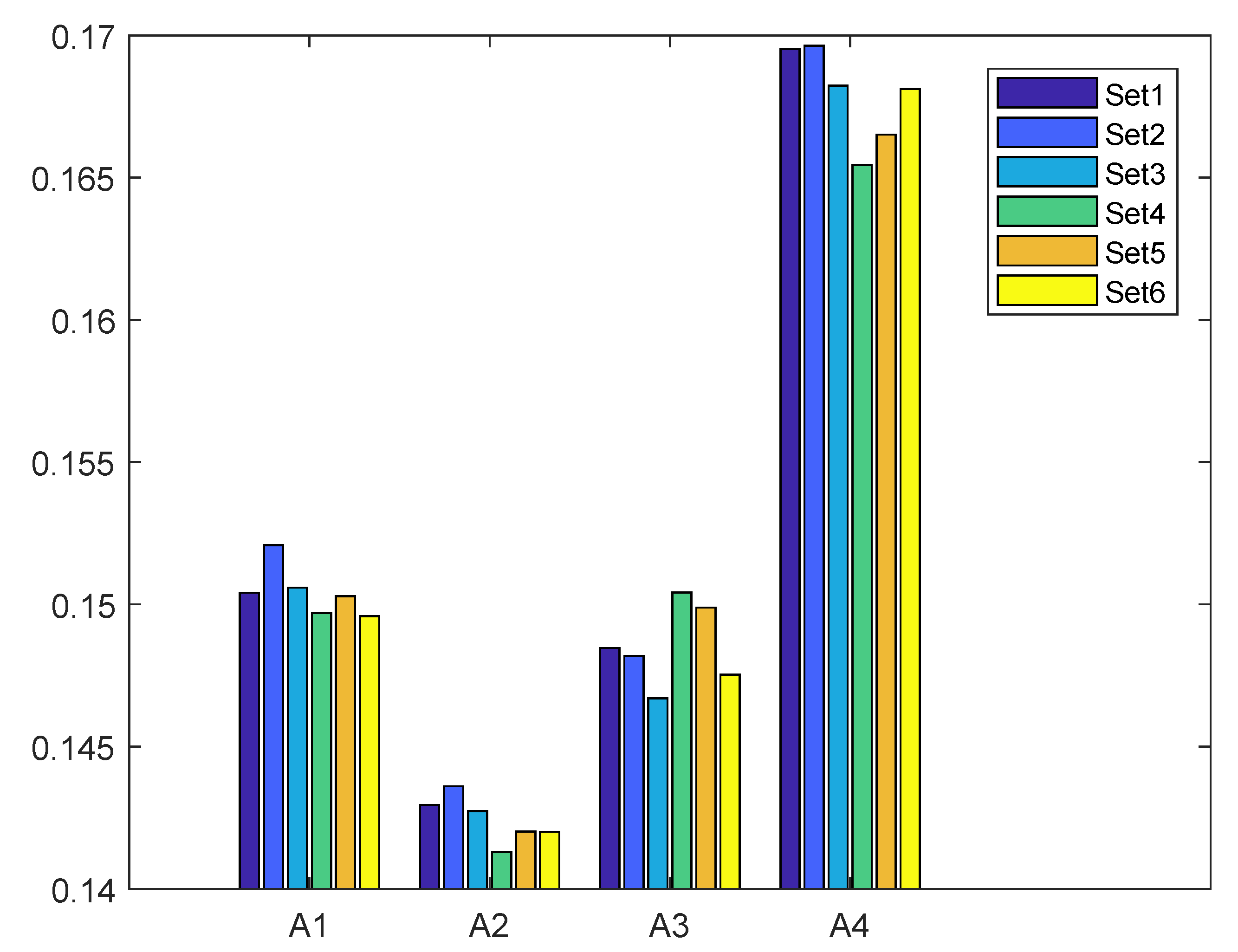
To study the robustness and stability of the proposed method, it is necessary to analyze the sensitivity of the subjective weight of the criteria. Since the importance evaluation of the criteria is determined by the decision-maker subjectively, there must be human errors caused by the subjective evaluation. Therefore, six groups of importance weights of the criteria are randomly selected, as shown in

Table 15. The generated importance weights of the criteria.

Sets	${\mathit{C}}_1$	${\mathit{C}}_2$	${\mathit{C}}_3$	${\mathit{C}}_4$	${\mathit{C}}_5$
Set 1	(0.8, 0.9, 1.0, 1.0)	(0.5, 0.6, 0.7, 0.8)	(0.4, 0.5, 0.5, 0.6)	(0.2, 0.3, 0.4, 0.5)	(0.1, 0.2, 0.2, 0.3)
Set 2	(0.1, 0.2, 0.2, 0.3)	(0.8, 0.9, 1.0, 1.0)	(0.5, 0.6, 0.7, 0.8)	(0.4, 0.5, 0.5, 0.6)	(0.2, 0.3, 0.4, 0.5)
Set 3	(0.2, 0.3, 0.4, 0.5)	(0.1, 0.2, 0.2, 0.3)	(0.8, 0.9, 1.0, 1.0)	(0.5, 0.6, 0.7, 0.8)	(0.4, 0.5, 0.5, 0.6)
Set 4	(0.4, 0.5, 0.5, 0.6)	(0.2, 0.3, 0.4, 0.5)	(0.1, 0.2, 0.2, 0.3)	(0.8, 0.9, 1.0, 1.0)	(0.5, 0.6, 0.7, 0.8)
Set 5	(0.5, 0.6, 0.7, 0.8)	(0.4, 0.5, 0.5, 0.6)	(0.2, 0.3, 0.4, 0.5)	(0.1, 0.2, 0.2, 0.3)	(0.8, 0.9, 1.0, 1.0)
Set 6	(0.7, 0.8, 0.8, 0.9)	(0.1, 0.2, 0.2, 0.3)	(0.8, 0.9, 1.0, 1.0)	(0.1, 0.2, 0.2, 0.3)	(0.7, 0.8, 0.8, 0.9)

. The belief values corresponding to the alternative schemes are calculated, and the best scheme is selected.

According to six groups of importance weights of the criteria, the belief values of each alternative are calculated, as shown in

Table 16. Sensitivity analysis of the subjective weights of the criteria.

$\mathit{m}\left(\mathit{C}\right)$	Set 1	Set 2	Set 3	Set 4	Set 5	Set 6
A1	0.1504	0.1521	0.1506	0.1497	0.1503	0.1496
A2	0.1429	0.1436	0.1427	0.1413	0.1420	0.1420
A3	0.1485	0.1482	0.1467	0.1504	0.1499	0.1475
A4	0.1695	0.1696	0.1682	0.1654	0.1665	0.1681

and Figure 2.

Except that the alternative ranking of Set 4 is $A_4$ > $A_3$ > $A_1$ > $A_2$, the alternative ranking calculated by other groups is $A_4$ > $A_1$ > $A_3$ > $A_2$, indicating that the change of belief value of alternative is basically stable against the variation in importance weights of the criteria. The criteria ranking corresponding to Set 4 is $C_4$ > $C_5$ > $C_1$ > $C_2$ > $C_3$ according to the relative importance, which results in the lowest evaluation weighting coefficient based on $C_3$ criterion and affects the final $A_1$ and $A_3$ ranking results, which shows that the method is sensitive to the variation in subjective weight. Because the proposed method is affected by some subjective weight changes, it can result in human errors in the decision results. Therefore, the proposed method is suitable for a decision-making environment with less human error.

In addition, as shown in

Table 17. Ranking order under the variation of criteria weights.

Sets	1	2	3	4
Set 1	$A_4$	$A_1$	$A_3$	$A_2$
Set 2	$A_4$	$A_1$	$A_3$	$A_2$
Set 3	$A_4$	$A_1$	$A_3$	$A_2$
Set 4	$A_4$	$A_3$	$A_1$	$A_2$
Set 5	$A_4$	$A_1$	$A_3$	$A_2$
Set 6	$A_4$	$A_1$	$A_3$	$A_2$

, no matter how the relative importance of the criteria changes, the best scheme is always $A_4$, which confirms the effectiveness of the method, and shows that the proposed method is effective for the correction of subjective errors.

5. Conclusions

This paper presents a weights-determining method in MCDM based on negation of probability distribution under uncertain environment. The main contribution of this paper is the combination of probability distribution negation and evidence fusion, which provides a new way to solve MCDM problems. While inheriting the advantage of EFMCDM in quantitative description of the uncertainty, through quantitative evaluation of the fuzzy degree of the criteria, to a certain extent, the error of experts’ subjective evaluation of each criterion is corrected to improve the decision-making level.

In the future work, the proposed method presents a new improvement scheme for the multi-attribute decision-making problem, which can be widely used in all aspects of life, e.g., supplier selection. In addition, on the premise of ensuring the correctness of the best scheme, we intend to further eliminate the influence of human subjective error on the order of alternatives.

References

1. Yang, G.L.; Yang, J.B.; Xu, D.L.; Khoveyni, M. A three-stage hybrid approach for weight assignment in MADM. Omega 2017, 71, 93–105. [Google Scholar] [CrossRef]
2. Chatterjee, K.; Zavadskas, E.; Tamošaitienė, J.; Adhikary, K.; Kar, S. A hybrid MCDM technique for risk management in construction projects. Symmetry 2018, 10, 46. [Google Scholar] [CrossRef] [Green Version]
3. Gerogiannis, V.C.; Karageorgos, A.; Liu, L.; Tjortjis, C. Personalised fuzzy recommendation for high involvement products. In Proceedings of the 2013 IEEE International Conference on Systems, Man, and Cybernetics, Manchester, UK, 13–16 October 2013; pp. 4884–4890. [Google Scholar]
4. Gou, X.; Liao, H.; Xu, Z.; Min, R.; Herrera, F. Group decision making with double hierarchy hesitant fuzzy linguistic preference relations: Consistency based measures, index and repairing algorithms and decision model. Inf. Sci. 2019, 489, 93–112. [Google Scholar] [CrossRef]
5. Mardani, A.; Nilashi, M.; Zavadskas, E.K.; Awang, S.R.; Zare, H.; Jamal, N.M. Decision Making Methods Based on Fuzzy Aggregation Operators: Three Decades Review from 1986 to 2017. Int. J. Inf. Technol. Decis. Mak. 2018, 17, 391–466. [Google Scholar] [CrossRef]
6. Yager, R.R. Fuzzy rule bases with generalized belief structure inputs. Eng. Appl. Artif. Intell. 2018, 72, 93–98. [Google Scholar] [CrossRef]
7. Seiti, H.; Hafezalkotob, A.; Fattahi, R. Extending a pessimistic–optimistic fuzzy information axiom based approach considering acceptable risk: Application in the selection of maintenance strategy. Appl. Soft Comput. 2018, 67, 895–909. [Google Scholar] [CrossRef]
8. Zhou, Q.; Mo, H.; Deng, Y. A New Divergence Measure of Pythagorean Fuzzy Sets Based on Belief Function and Its Application in Medical Diagnosis. Mathematics 2020, 8, 142. [Google Scholar] [CrossRef] [Green Version]
9. Pan, Y.; Zhang, L.; Li, Z.; Ding, L. Improved Fuzzy Bayesian Network-Based Risk Analysis With Interval-Valued Fuzzy Sets and D-S Evidence Theory. IEEE Trans. Fuzzy Syst. 2019. [Google Scholar] [CrossRef]
10. Gou, X.; Xu, Z.; Herrera, F. Consensus reaching process for large-scale group decision making with double hierarchy hesitant fuzzy linguistic preference relations. Knowl.-Based Syst. 2018, 157, 20–33. [Google Scholar] [CrossRef]
11. Cao, Z.; Lin, C.T.; Lai, K.L.; Ko, L.W.; King, J.T.; Liao, K.K.; Fuh, J.L.; Wang, S.J. Extraction of SSVEPs-based Inherent fuzzy entropy using a wearable headband EEG in migraine patients. IEEE Trans. Fuzzy Syst. 2019. [Google Scholar] [CrossRef] [Green Version]
12. Feng, F.; Fujita, H.; Ali, M.I.; Yager, R.R.; Liu, X. Another view on generalized intuitionistic fuzzy soft sets and related multiattribute decision making methods. IEEE Trans. Fuzzy Syst. 2018, 27, 474–488. [Google Scholar] [CrossRef]
13. Song, Y.; Deng, Y. A new soft likelihood function based on power ordered weighted average operator. Int. J. Intell. Syst. 2019, 34, 2988–2999. [Google Scholar] [CrossRef]
14. Feng, F.; Cho, J.; Pedrycz, W.; Fujita, H.; Herawan, T. Soft set based association rule mining. Knowl.-Based Syst. 2016, 111, 268–282. [Google Scholar] [CrossRef]
15. Yager, R.R. Interval valued entropies for Dempster–Shafer structures. Knowl.-Based Syst. 2018, 161, 390–397. [Google Scholar] [CrossRef]
16. Liu, Z.; Liu, Y.; Dezert, J.; Cuzzolin, F. Evidence combination based on credal belief redistribution for pattern classification. IEEE Trans. Fuzzy Syst. 2019. [Google Scholar] [CrossRef] [Green Version]
17. Gao, S.; Deng, Y. An evidential evaluation of nuclear safeguards. Int. J. Distrib. Sens. Netw. 2020, 16. [Google Scholar] [CrossRef] [Green Version]
18. Mo, H.; Deng, Y. Identifying node importance based on evidence theory in complex networks. Phys. A Stat. Mech. Its Appl. 2019. [Google Scholar] [CrossRef]
19. Song, Y.; Wang, X.; Zhu, J.; Lei, L. Sensor dynamic reliability evaluation based on evidence theory and intuitionistic fuzzy sets. Appl. Intell. 2018, 48, 3950–3962. [Google Scholar] [CrossRef]
20. Jiang, W.; Cao, Y.; Deng, X. A novel Z-network model based on Bayesian network and Z-number. IEEE Trans. Fuzzy Syst. 2019. [Google Scholar] [CrossRef]
21. Liu, P.; Zhang, X. A Multicriteria Decision-Making Approach with Linguistic D Numbers Based on the Choquet Integral. Cognit. Comput. 2019. [Google Scholar] [CrossRef]
22. Mo, H.; Deng, Y. An evaluation for sustainable mobility extended by D numbers. Technol. Econ. Dev. Econ. 2019, 25, 802–819. [Google Scholar] [CrossRef]
23. Wei, B.; Xiao, F.; Shi, Y. Synchronization in Kuramoto Oscillator Networks With Sampled-Data Updating Law. IEEE Trans. Cybern. 2019, 1–9. [Google Scholar] [CrossRef] [PubMed]
24. Xu, P.; Zhang, R.; Deng, Y. A Novel Visibility Graph Transformation of Time Series into Weighted Networks. Chaos Solitons Fractals 2018, 117, 201–208. [Google Scholar] [CrossRef]
25. Wei, B.; Xiao, F.; Shi, Y. Fully Distributed Synchronization of Dynamic Networked Systems with Adaptive Nonlinear Couplings. IEEE Trans. Cybern. 2019, 1–9. [Google Scholar] [CrossRef]
26. Qian, H.M.; Huang, H.Z.; Li, Y.F. A novel single-loop procedure for time-variant reliability analysis based on Kriging model. Appl. Math. Model. 2019, 75, 735–748. [Google Scholar] [CrossRef]
27. Liao, H.; Mi, X.; Xu, Z. A survey of decision-making methods with probabilistic linguistic information: Bibliometrics, preliminaries, methodologies, applications and future directions. Fuzzy Optim. Decis. Mak. 2019. [Google Scholar] [CrossRef]
28. Liao, H.; Wu, X. DNMA: A double normalization-based multiple aggregation method for multi-expert multi-criteria decision making. Omega 2019. [Google Scholar] [CrossRef]
29. Fei, L.; Xia, J.; Feng, Y.; Liu, L. An ELECTRE-based multiple criteria decision making method for supplier selection using Dempster-Shafer theory. IEEE Access 2019, 7, 84701–84716. [Google Scholar] [CrossRef]
30. Zhou, M.; Liu, X.B.; Chen, Y.W.; Qian, X.F.; Yang, J.B.; Wu, J. Assignment of attribute weights with belief distributions for MADM under uncertainties. Knowl.-Based Syst. 2019. [Google Scholar] [CrossRef]
31. Fu, C.; Xu, D.L. Determining attribute weights to improve solution reliability and its application to selecting leading industries. Ann. Oper. Res. 2016, 245, 401–426. [Google Scholar] [CrossRef]
32. Zhou, M.; Liu, X.B.; Chen, Y.W.; Yang, J.B. Evidential reasoning rule for MADM with both weights and reliabilities in group decision making. Knowl.-Based Syst. 2018, 143, 142–161. [Google Scholar] [CrossRef]
33. Xu, Z. An overview of methods for determining OWA weights. Int. J. Intell. Syst. 2005, 20, 843–865. [Google Scholar] [CrossRef]
34. Lamata, M.T.; Pérez, E.C. Obtaining OWA operators starting from a linear order and preference quantifiers. Int. J. Intell. Syst. 2012, 27, 242–258. [Google Scholar] [CrossRef]
35. Gerogiannis, V.C.; Fitsilis, P.; Kameas, A.D. Using a combined intuitionistic fuzzy set-TOPSIS method for evaluating project and portfolio management information systems. In Artificial Intelligence Applications and Innovations; Springer: Berlin/Heidelberg, Germany, 2011; pp. 67–81. [Google Scholar]
36. Fei, L.; Feng, Y.; Liu, L. Evidence combination using OWA-based soft likelihood functions. Int. J. Intell. Syst. 2019, 34, 2269–2290. [Google Scholar] [CrossRef]
37. Srivastava, A.; Maheshwari, S. Some new properties of negation of a probability distribution. Int. J. Intell. Syst. 2018, 33, 1133–1145. [Google Scholar] [CrossRef]
38. Srivastava, A.; Kaur, L. Uncertainty and negation–Information theoretic applications. Int. J. Intell. Syst. 2019, 34, 1248–1260. [Google Scholar] [CrossRef]
39. Luo, Z.; Deng, Y. A matrix method of basic belief assignment’s negation in Dempster-Shafer theory. IEEE Trans. Fuzzy Syst. 2019, 27. [Google Scholar] [CrossRef]
40. Xie, K.; Xiao, F. Negation of Belief Function Based on the Total Uncertainty Measure. Entropy 2019, 21, 73. [Google Scholar] [CrossRef] [Green Version]
41. Zhang, J.; Liu, R.; Zhang, J.; Kang, B. Extension of Yager’s negation of a probability distribution based on Tsallis entropy. Int. J. Intell. Syst. 2020, 35, 72–84. [Google Scholar] [CrossRef]
42. Xiao, F. EFMCDM: Evidential fuzzy multicriteria decision making based on belief entropy. IEEE Trans. Fuzzy Syst. 2019. [Google Scholar] [CrossRef]
43. Yager, R.R. On the maximum entropy negation of a probability distribution. IEEE Trans. Fuzzy Syst. 2014, 23, 1899–1902. [Google Scholar] [CrossRef]
44. Wang, T.; Wang, J.; Ming, J.; Sun, Z.; Wei, C.; Lu, C.; Pérez-Jiménez, M.J. Application of neural-like P systems with state values for power coordination of photovoltaic/battery microgrids. IEEE Access 2018, 6, 46630–46642. [Google Scholar] [CrossRef]
45. Song, Y.; Fu, Q.; Wang, Y.F.; Wang, X. Divergence-based cross entropy and uncertainty measures of Atanassov’s intuitionistic fuzzy sets with their application in decision making. Appl. Soft Comput. 2019, 84, 1–15. [Google Scholar] [CrossRef]
46. Zhou, D.; Al-Durra, A.; Zhang, K.; Ravey, A.; Gao, F. A Robust Prognostic Indicator for Renewable Energy Technologies: A Novel Error Correction Grey Prediction Model. IEEE Trans. Ind. Electron 2019, 66, 9312–9325. [Google Scholar] [CrossRef]
47. Wang, T.; Wei, X.; Huang, T.; Wang, J.; Valencia-Cabrera, L.; Fan, Z.; Pérez-Jiménez, M.J. Cascading Failures Analysis Considering Extreme Virus Propagation of Cyber-Physical Systems in Smart Grids. Complexity 2019, 2019. [Google Scholar] [CrossRef] [Green Version]
48. Liu, W.; Wang, T.; Zang, T.; Huang, Z.; Wang, J.; Huang, T.; Wei, X.; Li, C. A fault diagnosis method for power transmission networks based on spiking neural P systems with self-updating rules considering biological apoptosis mechanism. Complexity 2019, 2019. [Google Scholar] [CrossRef] [Green Version]
49. Wang, T.; Wei, X.; Huang, T.; Wang, J.; Peng, H.; Pérez-Jiménez, M.J.; Valencia-Cabrera, L. Modeling fault propagation paths in power systems: A new framework based on event SNP systems with neurotransmitter concentration. IEEE Access 2019, 7, 12798–12808. [Google Scholar] [CrossRef]
50. Yuan, R.; Tang, M.; Wang, H.; Li, H. A Reliability Analysis Method of Accelerated Performance Degradation Based on Bayesian Strategy. IEEE Access 2019, 7, 169047–169054. [Google Scholar] [CrossRef]
51. Li, H.; Yuan, R.; Fu, J. A reliability modeling for multi-component systems considering random shocks and multistate degradation. IEEE Access 2019, 7, 168805–168814. [Google Scholar] [CrossRef]
52. Seiti, H.; Tagipour, R.; Hafezalkotob, A.; Asgari, F. Maintenance strategy selection with risky evaluations using RAHP. J. Multi-Crit. Decis. Anal. 2017, 24, 257–274. [Google Scholar] [CrossRef]
53. Fang, R.; Liao, H.; Yang, J.B.; Xu, D.L. Generalised probabilistic linguistic evidential reasoning approach for multi-criteria decision-making under uncertainty. J. Oper. Res. Soc. 2019. [Google Scholar] [CrossRef]
54. Zhou, M.; Liu, X.; Yang, J. Evidential reasoning approach for MADM based on incomplete interval value. J. Intell. Fuzzy Syst. 2017, 33, 3707–3721. [Google Scholar] [CrossRef] [Green Version]
55. Cao, Z.; Lin, C.T. Inherent fuzzy entropy for the improvement of EEG complexity evaluation. IEEE Trans. Fuzzy Syst. 2018, 26, 1032–1035. [Google Scholar] [CrossRef] [Green Version]
56. Gao, X.; Liu, F.; Pan, L.; Deng, Y.; Tsai, S.B. Uncertainty measure based on Tsallis entropy in evidence theory. Int. J. Intell. Syst. 2019, 34, 3105–3120. [Google Scholar] [CrossRef]
57. Cao, Z.; Chuang, C.H.; King, J.K.; Lin, C.T. Multi-channel EEG recordings during a sustained-attention driving task. Sci. Data 2019, 6. [Google Scholar] [CrossRef] [PubMed] [Green Version]
58. Jiang, W.; Zhang, Z.; Deng, X. A Novel Failure Mode and Effects Analysis Method Based on Fuzzy Evidential Reasoning Rules. IEEE Access 2019, 7, 113605–113615. [Google Scholar] [CrossRef]
59. Liu, B.; Deng, Y. Risk Evaluation in Failure Mode and Effects Analysis Based on D Numbers Theory. Int. J. Comput. Commun. Control 2019, 14, 672–691. [Google Scholar]
60. Seiti, H.; Hafezalkotob, A. Developing the R-TOPSIS methodology for risk-based preventive maintenance planning: A case study in rolling mill company. Comput. Ind. Eng. 2019. [Google Scholar] [CrossRef]
61. Liu, Z.; Pan, Q.; Dezert, J.; Han, J.W.; He, Y. Classifier fusion with contextual reliability evaluation. IEEE Trans. Cybern. 2018, 48, 1605–1618. [Google Scholar] [CrossRef]
62. Fan, C.l.; Song, Y.; Lei, L.; Wang, X.; Bai, S. Evidence reasoning for temporal uncertain information based on relative reliability evaluation. Expert Syst. Appl. 2018, 113, 264–276. [Google Scholar] [CrossRef]
63. Xu, X.; Zheng, J.; Yang, J.b.; Xu, D.l.; Chen, Y.w. Data classification using evidence reasoning rule. Knowl.-Based Syst. 2017, 116, 144–151. [Google Scholar] [CrossRef] [Green Version]
64. Xiao, F. Distance measure of intuitionistic fuzzy sets and its application in pattern classification. IEEE Trans. Syst. Man Cybern. Syst. 2019. [Google Scholar] [CrossRef]
65. Xiao, F.; Zhang, Z.; Abawajy, J. Workflow scheduling in distributed systems under fuzzy environment. J. Intell. Fuzzy Syst. 2019, 37, 5323–5333. [Google Scholar] [CrossRef]
66. Xu, X.; Xu, H.; Wen, C.; Li, J.; Hou, P.; Zhang, J. A belief rule-based evidence updating method for industrial alarm system design. Control Eng. Pract. 2018, 81, 73–84. [Google Scholar] [CrossRef]
67. Deng, X.; Jiang, W. Evaluating green supply chain management practices under fuzzy environment: A novel method based on D number theory. Int. J. Fuzzy Syst. 2019, 21, 1389–1402. [Google Scholar] [CrossRef]
68. Seiti, H.; Hafezalkotob, A.; Martínez, L. R-numbers, a new risk modeling associated with fuzzy numbers and its application to decision making. Inf. Sci. 2019, 483, 206–231. [Google Scholar] [CrossRef]
69. Dempster, A.P. Upper and lower probabilities induced by a multivalued mapping. In Classic Works of the Dempster-Shafer Theory of Belief Functions; Springer: Berlin/Heidelberg, Germany, 2008; pp. 57–72. [Google Scholar]
70. Shafer, G. A Mathematical Theory of Evidence; Princeton University Press: Princeton, NJ, USA, 1976; Volume 42. [Google Scholar]
71. Xiao, F. A new divergence measure for belief functions in D-S evidence theory for multisensor data fusion. Inf. Sci. 2019. [Google Scholar] [CrossRef]
72. Song, Y.; Deng, Y. Divergence measure of belief function and its application in data fusion. IEEE Access 2019, 7, 107465–107472. [Google Scholar] [CrossRef]
73. Liu, Y.; Jiang, W. A new distance measure of interval-valued intuitionistic fuzzy sets and its application in decision making. Soft Comput. 2019, 23. [Google Scholar] [CrossRef]
74. Pan, L.; Deng, Y. An association coefficient of belief function and its application in target recognition system. Int. J. Intell. Syst. 2020, 35, 85–104. [Google Scholar] [CrossRef]
75. Jiang, W.; Huang, C.; Deng, X. A new probability transformation method based on a correlation coefficient of belief functions. Int. J. Intell. Syst. 2019, 34, 1337–1347. [Google Scholar] [CrossRef]
76. Li, M.; Xu, H.; Deng, Y. Evidential Decision Tree Based on Belief Entropy. Entropy 2019, 21, 897. [Google Scholar] [CrossRef] [Green Version]
77. Kang, B.; Deng, Y. The maximum Deng entropy. IEEE Access 2019, 7, 120758–120765. [Google Scholar] [CrossRef]
78. Liu, F.; Gao, X.; Zhao, J.; Deng, Y. Generalized Belief Entropy and Its Application in Identifying Conflict Evidence. IEEE Access 2019, 7, 126625–126633. [Google Scholar] [CrossRef]
79. Su, X.; Li, L.; Qian, H.; Sankaran, M.; Deng, Y. A new rule to combine dependent bodies of evidence. Soft Comput. 2019, 23, 9793–9799. [Google Scholar] [CrossRef]
80. Gao, X.; Deng, Y. Quantum Model of Mass Function. Int. J. Intell. Syst. 2020, 35, 267–282. [Google Scholar] [CrossRef]
81. Li, Y.; Deng, Y. Intuitionistic Evidence Sets. IEEE Access 2019, 7, 106417–106426. [Google Scholar] [CrossRef]
Figure 1. The procedure of proposed method.
Mathematics 08 00191 g001
Figure 2. Sensitivity analysis of the subjective weights of the criteria.
Mathematics 08 00191 g002