A New Explicit Magnus Expansion for Nonlinear Stochastic Differential Equations

Abstract

In this paper, based on the iterative technique, a new explicit Magnus expansion is proposed for the nonlinear stochastic equation $dy=A(t,y)ydt+B(t,y)y\circ dW.$ One of the most important features of the explicit Magnus method is that it can preserve the positivity of the solution for the above stochastic differential equation. We study the explicit Magnus method in which the drift term only satisfies the one-sided Lipschitz condition, and discuss the numerical truncated algorithms. Numerical simulation results are also given to support the theoretical predictions.

1. Introduction

Stochastic differential equations (SDE) have been widely applied in describing and understanding the random phenomena in different areas, such as biology, chemical reaction engineering, physics, finance and so on. The stochastic differential equations can also be applied in 5G wireless networks to address the problem of joint transmission power [1,2], and the novel frameworks were showed in [3,4]. However, in most cases, explicit solutions of stochastic differential equations are not easy to get. Therefore, it is necessary and important to exploit the algorithms for the stochastic differential equations. So far, there is a lot of literature on the numerical approximation of stochastic differential equations [5,6]. One kind of approximation which aims to preserve the essential properties of corresponding systems is getting more and more attention. For example, a conservative method for stochastic Hamiltonian systems with additive and multiplicative noise [7], the stochastic Lie group integrators [8]. In this paper, we will focus on the stochastic Magnus expansions [9].

As is well known, the deterministic Magnus expansion was first investigated by Magnus [10] in 1960s. This topic was further pursued in [11,12]. With the development of stochastic differential equations, the stochastic Magnus expansion got more and more attention when approximating solutions of linear and nonlinear stochastic differential equations [13,14].

The linear stochastic differential equation is as follows

$$dY(t)=A(t)Ydt+B(t)Y\circ dW(t),Y(0)=Y_0,$$

(1)

where $A(t)$ and $B(t)$ are $n\times n$ matrices, $W(t)$ is the standard Wiener process, $Y(t)$ is expressed by $Y(t)=exp(\Omega (t))Y_0$, where $\Omega (t)$ can be represented by an infinite series $\Omega (t)={\sum }_{k=1}^{\infty }{\Omega }_k(t)$, whose terms are linear combinations of multiple stochastic integrals.

For example, the first two terms are as follows,

$${\Omega }_1(t)={\int }_o^{t}A(t_1)d{t}_1+{\int }_0^{t}B(t_1)\circ dW(t_1),$$

(2)

$$\begin{array}{cc}\hfill {\Omega }_2(t)& =\frac{1}{2}{\int }_0^{t}d{t}_1{\int }_0^{t_1}d{t}_2[A(t_1),A(t_2)]+\frac{1}{2}{\int }_0^{t}d{t}_1{\int }_0^{t_1}\circ dW(t_2)[A(t_1),B(t_2)]\hfill \\ \hfill & +\frac{1}{2}{\int }_0^t\circ dW(t_1){\int }_0^{t_1}d{t}_2[B(t_1),A(t_2)]+\frac{1}{2}{\int }_0^t\circ dW(t_1){\int }_0^{t_1}\circ dW(t_2)[B(t_1),B(t_2)],\hfill \end{array}$$

(3)

where $[X,Y]=XY-YX$ is the matrix commutator of X and Y.

In this paper, we design explicit stochastic Magnus expansions [9] for the nonlinear equation

$$dy=A(t,y)ydt+B(t,y)y\circ dW,y(t_0)=y_0\in G,$$

(4)

$$A,B:R_{+}\times G\to g,$$

where G denotes a matrix Lie group, and g is the corresponding Lie algebra of G. The Equation (4) has lots of applications in the calculation of highly oscillatory systems of stochastic differential equations, Hamiltonian dynamics and finance engineering. It is necessary to construct efficient numerical integrators for the above equation. The general procedure of devising Magnus expansions for the above stochastic Equation (4) was obtained by applying Picard’s iteration to the new derived stochastic differential equation with the Lie algebra, which is an extension of the stochastic case [11]. G. Lord, J.A. Malham and A.wiese [14] proposed the stochastic Magnus integrators using different techniques.

With the application of the stochastic Magnus methods, we can recapture some main features of the stochastic differential Equations (4) successfully. When Equation (4) is used to describe the asset pricing model in finance, the positivity of the solution is a very important factor to be maintained in the numerical simulation. This task can be accomplished by the nonlinear Magnus methods. We also notice that lots of works [15,16] have dealt with this issue using the methods of balancing and dominating. However, the Magnus methods using the Lie group methods are essentially different from the aforementioned methods. If Equation (4) has an almost sure exponential stable solution, it is necessary to construct numerical methods to preserve this property. The numerical methods which preserve the exponential stability usually have long-time numerical behavior. We prove that the explicit Magnus methods succeed in reproducing the almost sure exponential stability for the stochastic differential Equation (4) with a one-sided Lipschitz condition. Numerical simulation results are also given to support the theoretical predictions.

This paper is organized as follows. We introduce and discuss the nonlinear Magnus in Section 2. The numerical truncated algorithms are discussed in Section 3. Then several numerical applications and experiments strongly support the theoretical analysis. In Section 4, we present the applications in the highly oscillating nonlinear stochastic differential equations. Section 5 consists of the simulations of processes for the dynamic asset pricing models. In Section 6, we show that the explicit Magnus simulation can preserve the almost sure stability and numerical experiments are presented to support the analysis.

Notation

In this paper, $(\Omega ,\mathcal{F},{\left\{{\mathcal{F}}_t\right\}}_{t\ge 0},\mathbb{P})$ is the complete probability space with the filtration ${\left\{{\mathcal{F}}_t\right\}}_{t\ge 0}$. $W(t)$ is the scalar Brownian motion defined on the probability space. $\circ dW(t)$ denotes the Stratonovich integral and $dW(t)$ denotes the Itô integral. $[X,Y]=XY-YX$ is the matrix commutator of X and Y. A and B are $n\times n$ matrices and smooth in the domain, $W(t)$ is the standard Wiener process and $\mathbb{E}|y_0{|}^2<\propto$.

2. The Nonlinear Stochastic Magnus Expansion

In this section, we consider a stochastic differential Equation (4).

Here, A and B have uniformly bounded partial derivatives, $A(t,y)y$ and $B(t,y)y$ satisfy the global Lipschtiz conditions. Therefore, Equation (4) has a unique strong solution [17].

The solution of Equation (4) is presented as follows

$$Y(t)=exp(\Omega (t))Y_0,$$

(5)

and

$$d\Omega (t)={\Omega }_1(t)dt+{\Omega }_2(t)\circ dW.$$

(6)

Combining (5) with (4), we have

$$dY=A(t,Y)Ydt+B(t,Y)Y\circ dW(t)=dexp(\Omega (t))Y_0=\sum _{k=1}^{\infty }\frac{1}{k!}\sum _{j=1}^k\Omega {(t)}^{j-1}d\Omega (t)\Omega {(t)}^{k-j}{Y}_0.$$

(7)

Equation (7) holds since the integral is in the Stratnovitch sense.

Inserting (6) into (7), we can get

$$\sum _{k=1}^{\infty }\frac{1}{k!}\sum _{j=1}^k\Omega {(t)}^{j-1}{\Omega }_1(t)\Omega {(t)}^{k-j}=A(t,exp(\Omega (t))Y_0)exp(\Omega (t)),$$

(8)

$$\sum _{k=1}^{\infty }\frac{1}{k!}\sum _{j=1}^k\Omega {(t)}^{j-1}{\Omega }_2(t)\Omega {(t)}^{k-j}=B(t,exp(\Omega (t))Y_0)exp(\Omega (t)).$$

(9)

According to Equation (8), we obtain

$$\begin{array}{cc}\hfill A(t,exp(\Omega (t))Y_0)& =\sum _{k=1}^{\infty }\frac{1}{k!}(\sum _{j=1}^k\Omega {(t)}^{j-1}{\Omega }_1(t)\Omega {(t)}^{k-j})exp(-\Omega (t))\hfill \\ \hfill & =\sum _{k=1}^{\infty }\frac{1}{k!}(\sum _{j=1}^k\Omega {(t)}^{j-1}{\Omega }_1(t)\Omega {(t)}^{k-j})[\sum _{l=0}^{\infty }\frac{{(-1)}^l}{l!}\Omega {(t)}^l]\hfill \\ \hfill & =\sum _{l=1}^{\infty }\frac{{(-1)}^l}{l!}\sum _{j=1}^l[\sum _{k=j}^l{(-1)}^k\left(\begin{array}{c}l\\ k\end{array}\right)]\Omega {(t)}^{j-l}{\Omega }_1(t)\Omega {(t)}^{l-j}.\hfill \end{array}$$

(10)

It is not difficult to check that

$$\sum _{k=j}^l{(-1)}^k\left(\begin{array}{c}l\\ k\end{array}\right)={(-1)}^j\left(\begin{array}{c}l-1\\ j-1\end{array}\right),$$

(11)

and

$$\mathbf{ad}[{(\Omega (t))}^l,{\Omega }_1(t)]=\sum _{j=0}^l{(-1)}^{l-j}\left(\begin{array}{c}l\\ j\end{array}\right)\Omega {(t)}^j{\Omega }_1(t)\Omega {(t)}^{l-j},l\in {\mathbb{Z}}^{+},$$

(12)

where $\mathbf{ad}[p^0,q]=q$ and $\mathbf{ad}[p^k,q]=[p,\mathbf{ad}[p^{k-1},q]]$ for $k\in \mathbb{N}$.

Then it is true that

$$\sum _{l=0}^{\infty }\frac{1}{(l+1)!}\mathbf{ad}[\Omega {(t)}^l,{\Omega }_1(t)]=A(t,exp(\Omega (t))Y_0),$$

(13)

$$\sum _{l=0}^{\infty }\frac{1}{(l+1)!}\mathbf{ad}[\Omega {(t)}^l,{\Omega }_2(t)]=B(t,exp(\Omega (t))Y_0).$$

(14)

Equations (13) and (14) indicate that

$${\Omega }_1(t)=\sum _{m=0}^{\infty }{f}_m\mathbf{ad}[{\Omega }^m,A(t,exp(\Omega (t))Y_0)],$$

(15)

$${\Omega }_2(t)=\sum _{m=0}^{\infty }{f}_m\mathbf{ad}[{\Omega }^m(t),B(t,exp(\Omega (t))Y_0)],$$

(16)

where

$$d(z)=\frac{exp(z)-1}{z},$$

$$f_m=\sum _{m=0}^{\infty }{f}_m{z}^m=\frac{1}{d(z)}.$$

Finally, we get

$$\begin{array}{cc}\hfill d\Omega (t)& =\sum _{m=0}^{\infty }{f}_m\mathbf{ad}[{\Omega }^m(t),A(t,exp(\Omega (t))Y_0)]dt\hfill \\ \hfill & +\sum _{m=0}^{\infty }{f}_m\mathbf{ad}[{\Omega }^m(t),B(t,exp(\Omega (t))Y_0)]\circ dW(t).\hfill \end{array}$$

(17)

Then, applying the Picard’s iteration to (17), we obtain

$$\begin{array}{cc}\hfill {\Omega }^{(m+1)}(t)& ={\int }_0^t\sum _{k=0}^{\infty }\frac{B_k}{k!}\mathbf{ad}[{\Omega }^m{(t)}^k,A(s,exp({\Omega }^m(t))Y_0)]ds\hfill \\ \hfill & +{\int }_0^t\sum _{k=0}^{\infty }\frac{B_k}{k!}\mathbf{ad}[{\Omega }^m{(t)}^k,B(s,exp({\Omega }^m(t))Y_0)]\circ dW(s),m\ge 0.\hfill \end{array}$$

(18)

In order to get explicit numerical methods which can be implemented in the computer, we need to truncate the infinite series in (18). The iterate function series ${\Omega }^{(m+1)}(t)$ only reproduce the expansion of the solution $\Omega (t)$ up to certain orders in the mean-square sense.

For example, if $m=0$, we obtain

$${\Omega }^1(t)={\int }_0^{t}A(s,Y_0)ds+{\int }_0^{t}B(s,Y_0)\circ dW(s)=\Omega (t)+\mathcal{O}(t).$$

(19)

From

$$A(s,exp({\Omega }^1(s))Y_0)=A(0,Y_0)+\mathcal{O}(s),$$

$$B(s,exp({\Omega }^1(s))Y_0)=B(0,Y_0)+\mathcal{O}(s),$$

we can get

$$-\frac{1}{2}{\int }_0^t[{\Omega }^1(s),A(s,exp({\Omega }^1(s))Y_0)]ds=\mathcal{O}(t^3),$$

$$-\frac{1}{2}{\int }_0^t[{\Omega }^1(s),B(s,exp({\Omega }^1(s))Y_0)]\circ dW=\mathcal{O}(t^{2.5}).$$

Finally, we devise the following general Magnus expansion

$${\Omega }^1(t)={\int }_0^{t}A(s,Y_0)ds+{\int }_0^{t}B(s,Y_0)\circ dW(s),$$

(20)

$$\begin{array}{cc}\hfill {\Omega }^m(t)& =\sum _{k=0}^{m-2}{\int }_0^t\mathbf{ad}[{{\Omega }^{(m-1)}(t)}^k,A(s,exp({\Omega }^{(m-1)}(t))Y_0)]ds\hfill \\ \hfill & +\sum _{k=0}^{m-2}{\int }_0^t\mathbf{ad}[{{\Omega }^{(m-1)}(t)}^k,B(s,exp({\Omega }^{(m-1)}(t))Y_0)]\circ dW(s).\hfill \end{array}$$

(21)

Obviously, Equation (21) consists of a linear combination of multiple stochastic integrals of nested commutators. It is easy to prove that ${\Omega }^m(t)$ succeeds in reproducing the sum of the $\Omega (t)$ series with the Magnus expansion. This scheme is called an explicit stochastic Magnus expansion for the nonlinear stochastic differential equation.

Remark 1.

We let $\Omega (t)$ be the exact solution of the problem (17) and ${\Omega }^m(t)$ be the approximate solution given by (21).

It is true that

$$\Omega (t)-{\Omega }^m(t)=\mathcal{O}(t^{\frac{m}{2}}),$$

(22)

we can write the exact solution of Equation (17) as

$$\Omega (t)=\sum _{l=1}^{\infty }\sum _{J=(i_1,i_2,\cdots ,i_l),i_k\in (0,1)}{\int }_{{\Delta }^J[0,t]}\circ d{W}^J{\omega }^J.$$

where ${\omega }^{(0)}=A(Y_0)$, ${\omega }^{(1)}=B(Y_0)$, $d{W}^J=d{W}^{i_1}\circ d{W}^{i_2}\cdots \circ d{W}^{i_l}$, and

$$d{W}^{i_j}=\left\{\begin{array}{cc}dt,& i_j=0,\\ dW,& i_j=1.\end{array}\right.$$

$$\Omega (t)-{\Omega }^m(t)=\sum _{l=m+1}^{\infty }\sum _{J=(i_1,i_2,\cdots ,i_l),i_k\in (0,1)}{\int }_{{\Delta }^J[0,t]}\circ d{W}^J{\omega }^J.),$$

(23)

The general Magnus expansion is

$${\Omega }^m(t)=\sum _{k=0}^{m-2}{\int }_0^t\mathbf{ad}[{{\Omega }^{(m-1)}(t)}^k,A(s,exp({\Omega }^{(m-1)}(t))Y_0)]ds$$

$$+\sum _{k=0}^{m-2}{\int }_0^t\mathbf{ad}[{{\Omega }^{(m-1)}(t)}^k,B(s,exp({\Omega }^{(m-1)}(t))Y_0)]\circ dW(s)$$

Comparing the Taylor expansion of the ${\Omega }^m(t)$ with the expansion of $\Omega (t)$ [12], the conclusion is proven.

3. Numerical Schemes

In this section, we present a new way of constructing efficient numerical methods based on the nonlinear stochastic Magnus expansion. It should be mentioned that highly efficient schemes always involve multiple stochastic integrals. In most cases, however, the half-order approximation of ${\Omega }^1(t)$ (21) can only be exactly evaluated. In order to get higher order integrator, more complicated multiple stochastic integrals, which are hard to approximate, must be included.

We will investigate the schemes of order (mean-square order) $1/2$ and 1 concretely, and choose the quadrature rules with equispaced points along the interval $[t_n,t_n+h]$.

3.1. Methods of Order 1/2

When $m=1$, the expansion (21) turns into

$${\Omega }^1(t)={\int }_{t_n}^{t}A(s,Y_n)ds+{\int }_{t_n}^{t}B(s,Y_n)\circ dW(s).$$

(24)

Using the Taylor formula, we can get the expansion of the solution

$$y(t_n+h)=y(t_n)+A(t_n,y(t_n))y(t_n)h+B(t_n,y(t_n))y(t_n)\Delta W_n+R_n^1,$$

(25)

and the approximate solution can be expanded in the following form

$$\overline{y}(t_n+h)=exp({\Omega }^1(t_n+h))y(t_n)=y(t_n)+A(t_n,y(t_n))y(t_n)h+B(t_n,y(t_n))y(t_n)\Delta W_n+R_n^2,$$

(26)

where,

$$R_n^2={\int }_{t_n}^{t_n+h}{\int }_{t_n}^s\frac{\partial A}{\partial t}d{s}_{1}ds+{\int }_{t_n}^{t_n+h}{\int }_{t_n}^s\frac{\partial B}{\partial t}d{s}_1\circ dW(s)+B{(t_n,y(t_n))}^2\Delta W_n^2+\mathcal{O}(h^{3/2}).$$

It is easy to check that

$$\mathbb{E}|y(t_n+h)-\overline{y}(t_n+h)|=\mathcal{O}(h^{3/2}),$$

$$(\mathbb{E}|y(t_n+h)-\overline{y}(t_n+h){{|}^2)}^{1/2}=\mathcal{O}(h^1).$$

According to the Milstein mean-square convergence theorem [18], the strong convergence order is $1/2$.

Remark 2.

If ${\Omega }^1(t)$ cannot be evaluated exactly, we need to approximate it with a quadrature rule of order $1/2$.

For example, using the Euler method (see reference [19]), we can get

$${\Omega }^1(t)=A(t_n,Y_n)\Delta t+B(t_n,Y_n)\Delta W(t).$$

(27)

Notice that other numerical methods can also be used to approximate (24). we can get the strong convergence order is $1/2$.

3.2. Methods of Order 1

When $m=2$, the expansion (21) becomes

$${\Omega }^1(t)={\int }_{t_n}^{t}A(s,Y_n)ds+{\int }_{t_n}^{t}B(s,Y_n)\circ dW(s),$$

(28)

$${\Omega }^2(t)={\int }_{t_n}^{t}A(s,exp({\Omega }^1(s))Y_n)ds+{\int }_{t_n}^{t}B(s,exp({\Omega }^1(s))Y_n)\circ dW(s).$$

(29)

The proof of the convergence order is the same as the method of order $1/2$.

Remark 3.

Note that if (28) can be computed exactly, all that is required is to replace (29) with a quadrature of order 1. Using the stochastic Taylor expansion, we approximate ${\Omega }^2(t)$ in the following way

$${\Omega }^2(t)=A(t_n,Y_n)\Delta t+B(t_n,Y_n)\Delta W(t)+\frac{\partial B}{\partial y}(t_n,Y_n)B(t_n,Y_n)Y_n\Delta W{(t)}^2/2.$$

(30)

As a matter of fact, there is no need to compute (28) or (29) exactly. If we approximate (28) or (29) with the methods of order 1,

$${\Omega }^1(t)=A(t_n,Y_n)\Delta t+B(t_n,Y_n)\Delta W(t).$$

The convergence order will also be order 1.

4. Numerical Experiment for the Highly Oscillatory Nonlinear Stochastic Differential Equations

We consider the following stochastic system

$$dy=A(t,y)ydt+B(t,y)y\circ dW,y(0)=y_0,$$

(31)

where A and B are matrices, W is the Wiener process. It is supposed that the solution of (31) oscillates rapidly.

If A and B are commutative, in order to compute the value of $y(t)$, a new $Z(x)$ is considered,

$$y(t_n+x)=exp(xA(t_n,y_n)+W(x)B(t_n,y_n))Z(x).$$

(32)

$$y_n\approx y(t_n),t_{n+1}=t_n+h,$$

(33)

and

$$dZ(x)=\overline{A(x,Z(x))}Z(x)dx+\overline{B(x,Z(x))}Z(x)\circ dW(x),Z(0)=y_n,$$

(34)

$$\overline{A(x,Z(x))}=F^{-1}(x)[A(t_n+x,F(x)Z(x))-A(t_n,y_n)]F(x),$$

(35)

$$\overline{B(x,Z(x))}=F^{-1}(x)[B(t_n+x,F(x)Z(x))-B(t_n,y_n)]F(x),$$

(36)

where $F(x)=exp[xA(t_n,y_n)+W(x)B(t_n,y_n)]$, $B(0,Z(0))=0$.

We can consider $Z(x)$ as a correction of the solution provided by ${\Omega }^{[1]}$. For this reason, if Equation (34) is solved by the method of the nonlinear Magnus expansion, the errors corresponding will be much smaller than the previous algorithms [13,14].

When A and B are not commutative with each other, we have [20]

$$y(t_n+x)=exp(xA(t_n,y_n))exp(W(x)B(t_n,y_n))Z_1(x),$$

(37)

and

$$\begin{array}{cc}\hfill d{Z}_1(x)& =\overline{A_1(x,Z_1(x))}{Z}_1(x)dx+\overline{B_1(x,Z_1(x))}{Z}_1(x)\circ dW(t_n+x)\hfill \\ \hfill & -\overline{B_2(x,Z_1(x))}{Z}_1(x)\circ dW(x),Z_1(0)=y_n,\hfill \end{array}$$

(38)

with

$$\overline{A_1(x,Z_1(x))}=F_1^{-1}(x)[A(t_n+x,F_1(x)Z_1(x))-A(t_n,y_n)]F_1(x),$$

(39)

$$\overline{B_1(x,Z_1(x))}=F_1^{-1}(x)[B(t_n+x,F_1(x)Z_1(x))]F_1(x),$$

(40)

$$\overline{B_2(x,Z_1(x))}=F_1^{-1}(x)[B(t_n,F_1(x)Z_1(x))]F_1(x),$$

(41)

here, $F_1(x)=exp(xA(t_n,y_n))exp(W(x)B(t_n,y_n)).$

To illustrate the main feature of the nonlinear modified Magnus expansion, we consider a system

$$\ddot{y}+a(t,y,\dot{y})y+b(t,y,\dot{y})y\dot{W}=0,$$

(42)

where, W is the standard Wiener process.

If $\dot{y}=x$, Equation (42) becomes

$$dZ=A(t,Z)Zdt+B(t,Z)Z\circ dW,$$

(43)

$Z={(y,y^{{}^{\prime }})}^T$,

$$A(t,Z)=\left(\begin{array}{cc}0& 1\\ -a(t,Z)& 0\end{array}\right),$$

$$B(t,Z)=\left(\begin{array}{cc}0& 0\\ -b(t,Z)& 0\end{array}\right).$$

It is easy to check that A and B are not commutative. By the use of the scheme (37), we obtain the following scheme

$$exp(xA(t_n,Z_n))=\left(\begin{array}{cc}cos(x{\theta }_n)& {\theta }_n^{-1}sin(x{\theta }_n)\\ -{\theta }_{n}sin(x{\theta }_n)& cos(x{\theta }_n)\end{array}\right),$$

$$exp(W(x)A(t_n,Z_n))=\left(\begin{array}{cc}1& 0\\ -w(x)b(t_n,Z_n)& 1\end{array}\right),$$

$$F_1(x)=\left(\begin{array}{cc}cos(x{\theta }_n)-W(x){\theta }_n^{-1}b(t_n,Z_n)sin(x{\theta }_n)& {\theta }_n^{-1}sin(x{\theta }_n)\\ -{\theta }_{n}sin(x{\theta }_n)-W(x)b(t_n,Z_n)cos(x{\theta }_n)& cos(x{\theta }_n)\end{array}\right),$$

$$F_1^{-1}(x)=\left(\begin{array}{cc}cos(x{\theta }_n)-W(x){\theta }_n^{-1}b(t_n,Z_n)sin(x{\theta }_n)& -{\theta }_n^{-1}sin(x{\theta }_n)\\ {\theta }_{n}sin(x{\theta }_n)+W(x)b(t_n,Z_n)cos(x{\theta }_n)& cos(x{\theta }_n)\end{array}\right),$$

and

$$\begin{array}{cc}\hfill d{Z}_1(x)& =\overline{A_1(x,Z_1(x))}{Z}_1(x)dx+\overline{B_1(x,Z_1(x))}{Z}_1(x)\circ dW(t_n+x)\hfill \\ \hfill & -\overline{B_2(x,Z_1(x))}{Z}_1(x)\circ dW(x),Z_1(0)=y_n,\hfill \end{array}$$

(44)

where ${\overline{A}}_1$, ${\overline{B}}_1$, ${\overline{B}}_2$ are computed by (39), (40), (42) and ${\theta }_n=\sqrt{a(t_n,Z_n)}$.

Applying the scheme (27) to Equation (44), we get the algorithm

$$Z_1(x)=exp(B(t_n,y_n)(W(t_n+x)-W(t_n))+B(t_n,y_n)\Delta W(x))y_n.$$

(45)

Then, inserting (45) into (37), we can get the one-step approximate algorithm.

In Figure 1, we can see that the two points $(\pm 1,0)$ initially attract the noisy trajectories, and after some time, the trajectories switch to the other point which coincides with the tunneling phenomena described in [21].

5. Application to the Stochastic Differential Equations with Boundary Conditions

In this section, we will deal with the Itô-type stochastic differential equation

$$dx(t)=f(x(t))dt+\sigma (x(t))dw(t),x(0)=x_0\in \mathcal{D},$$

(46)

we assume Equation (46) is well-defined with a certain boundary condition, that is, $x(t)$ lies in the domain $\mathcal{D}$.

There are lots of works on the efficient approximate solution of (46) [15,16,22]. Most of them use the balancing or dominating technique to restrict the numerical solution to stay in the domain. In this paper, the proposed explicit nonlinear Magnus methods based on the stochastic Lie group are efficient at approximating the solutions of stochastic differential Equations (46) with unattainable boundary conditions. Our methods are really different from the methods proposed in [23].

In the following, we will approximate two types of finance models using the nonlinear stochastic Magnus methods.

Firstly, we study the financial model defined as:

$$dX(t)=a(b-X(t))dt+\sigma X^{r}dw(t).$$

(47)

This model has been widely used in financial engineering. For example, when $2ab>{\sigma }^2,r=\frac{1}{2}$, the solution is strictly positive. As well known, the traditional Euler method fails to preserve the positivity of the solution. We also notice that several methods such as the balanced implicit method (BIM) [22] have been proposed. The explicit or implicit Milstein method needs stepsize control [24]. In the following, we show that the nonlinear Magnus methods preserve the positivity independent of the stepsize.

For Equation (47), its equivalent Stratonovich form is defined as:

$$dX(t)=[a(b-X(t))-\frac{r{\sigma }^2}{2}{X}^{2r-1}]dt+\sigma X^r\circ dw(t).$$

(48)

To simulate the above equation, we split the system (48) into two subsystems

$$d{X}_1(t)=-a{X}_1(t)dt+\sigma X_1{(t)}^r\circ dw(t),$$

(49)

and

$$d{X}_2(t)=[ab-\frac{r{\sigma }^2}{2}{X}_2^{2r-1}]dt.$$

(50)

The system (49) is simulated with the nonlinear stochastic Magnus method and (50) is approximated with Euler method.

Combining the nonlinear Magnus method (27) and the Euler method, we obtain one step method on the interval $[t_n,t_{n+1}]$

$$\begin{array}{cc}\hfill {\Omega }_{n+1}^1& =-a\Delta t_n+\Delta w(h)\frac{\sigma }{{(X_1^n)}^{r-1}},\hfill \\ \hfill X_1^{n+1}& =exp({\Omega }_{n+1}^1)X_1^n,\hfill \\ \hfill X_2^{n+1}& =X_1^{n+1}+(ab-\frac{r{\sigma }^2}{2}{(X_1^{n+1})}^{2r-1})\Delta t_n.\hfill \end{array}$$

(51)

In the numerical experiments, we use the scheme (51) to simulate the financial models. When $r=0.5$, it is the famous interest rate model of Cox, Ingeesoll, and Ross (for more detail, see [16]).

Table 1. Numerical simulation for the equation $dX(t)=(1-X(t))dt+1.4\sqrt{X(t)}dW(t)$, the time interval: $[0,T]$, stepsize: $dT$, weight functions of balanced Milstein method (BMM): $d^0(x)=1+0.5\ast {1.4}^2,d^1(x)=0$, the number of simulated paths: 1500.

Time	Stepsize	Euler	Milstein	BMM	NLM
T=1	dT=1/2	27.35%	22.12%	0%	0%
	dT=1/4	26.35%	8.21%	0%	0%
	dT=1/16	17.35%	0.12%	0%	0%
T=4	dT=1/2	69.35%	53.45%	0%	0%
	dT=1/4	66.24%	18.48%	0%	0%
	dT=1/16	57.89%	2.45%	0%	0%
T=16	dT=1/2	98.67%	94.25%	0%	0%
	dT=1/4	96.56%	58.48%	0%	0%
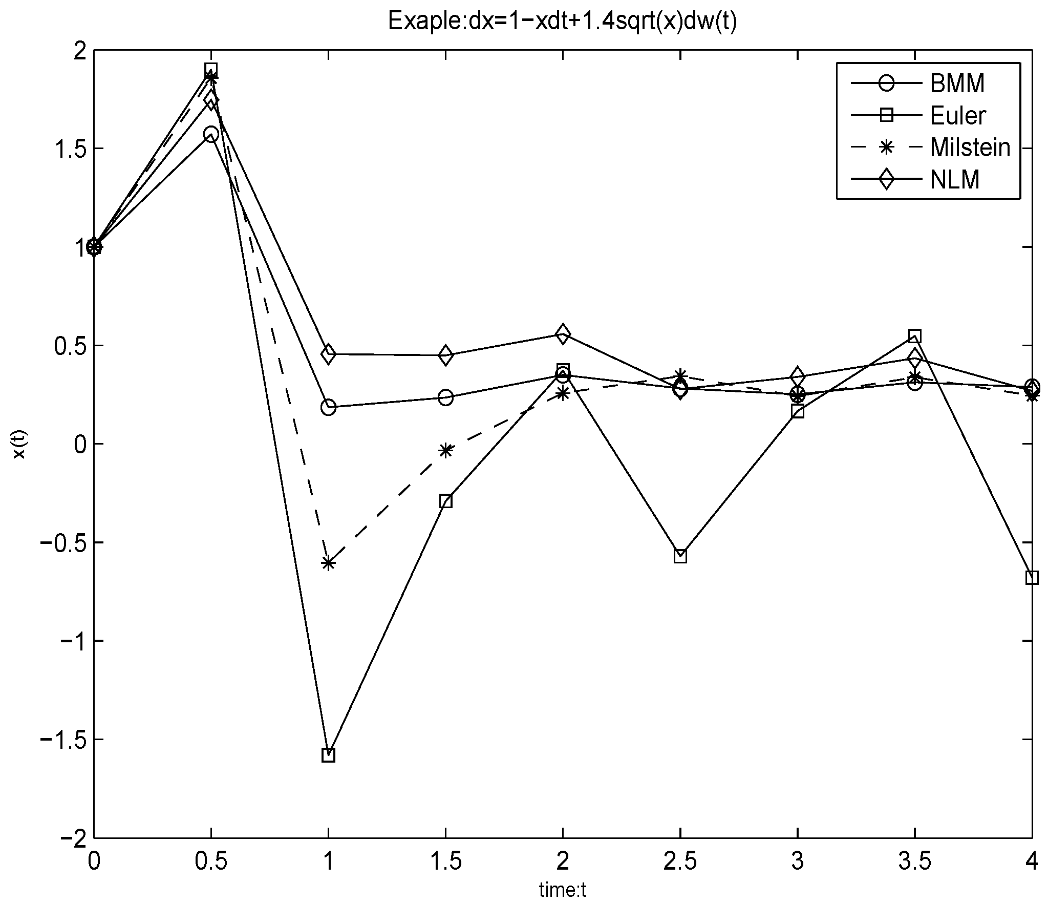
	dT=1/16	95.72%	9.08%	0%	0%

illustrates that both the Euler and the Milstein methods have a certain percentage of negative paths. When the stepsize decreases, the number of negative paths also decreases. However, the nonlinear Magnus method (NLM) is as good as the balanced Milstein method (BMM) preserving the positivity of the solution independent of time interval $[0,T]$ and the time stepsize $dT$.

In Figure 2 and Figure 3, we present the numerical simulations for two finance equations. We can see that both the Euler and the Milstein methods fail to preserve the positivity. However, the NLM is as good as the BMM and the BIM at preserving the positivity of the solution.

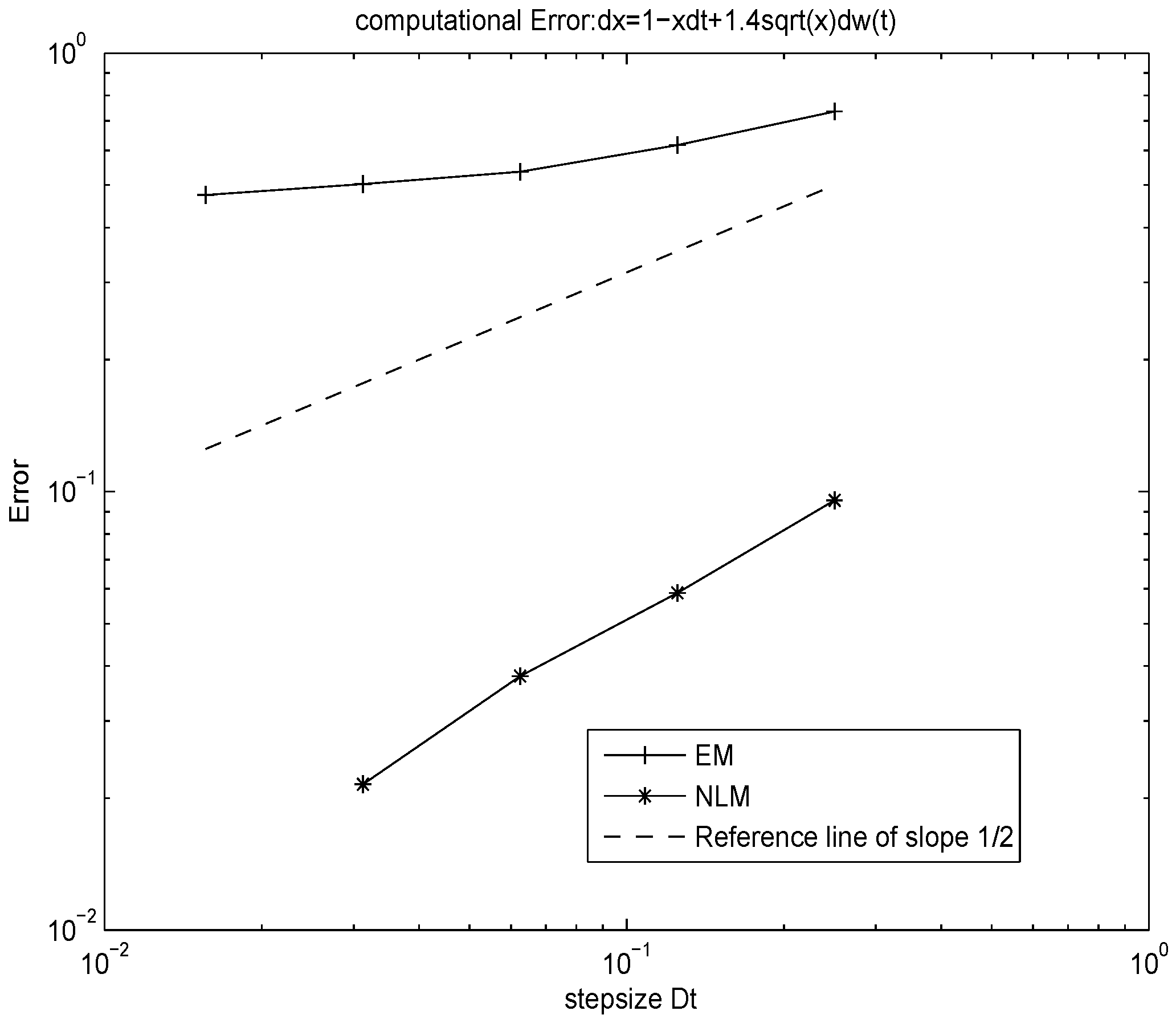
In Figure 4, we see that the explicit NLM which is of the order $1/2$ in mean square sense verifies the analysis in Section 3. In Figure 5, we can see clearly that the simulation is of the order 1 in mean square sense with the linear model, which is the same order as in the BMM.

6. Application to the Nonlinear Itô Scalar Stochastic Differential Equations

In this part, we will focus on the nonlinear Itô scalar stochastic differential equation

$$dy=a(y)ydt+\sigma ydW(t),$$

(52)

where $\sigma$ is independent of y. The Equation (52) satisfies the following conditions

$$\left|a(y)\right|\le K_i,\forall y\in \mathbb{R}with\left|y\right|\le i,$$

(53)

and

$$-\lambda =\underset{y\in \mathbb{R},y\ne 0}{sup}(a(y)-\frac{{\sigma }^2}{2})<0.$$

(54)

For convenience, we transform it into its Stratonovich form

$$dy=(a(y)-{\sigma }^2/2)ydt+\sigma y\circ dW(t).$$

(55)

Theorem 1.

Suppose that (52) satisfies (53) and (54), then the solution of (52) obeys

$$\underset{t->\infty }{lim}sup\frac{1}{t}log\left|y(t)\right|\le -\lambda a.s.$$

(56)

Proof. 

According to the Itô Taylor formula, we have

$$\begin{array}{cc}\hfill log(y^2)& =log(y{(0)}^2)+{\int }_0^{t}2{\sigma }^{2}dW(s)\hfill \\ \hfill & +{\int }_0^{t}2(a(y)-{\sigma }^2/2)dt.\hfill \end{array}$$

(57)

It is easy to prove that

$$\underset{t->\infty }{lim}\frac{{\int }_0^{t}2{\sigma }^{2}dW(s)}{t}=0,a.s.$$

(58)

By the use of the condition (54), we obtain

$$\frac{log(y{(t)}^2)}{2t}\le \frac{log(y{(0)}^2)}{2t}+\frac{{\int }_0^{t}2{\sigma }^{2}dW(s)}{2t}-\lambda .$$

(59)

Let $t->\infty$, (56) is proven.

It means that the solution of the stochastic differential equation is almost surely stable.

In the following, we will approximate the model using the nonlinear stochastic Magnus methods.

Applying (27) to Equation (55), we can get the approximation $Y_k\approx Y(k\Delta t)$ with $Y_0=y(0)$,

$$Y_{k+1}=exp((a(Y_k)-{\sigma }^2/2)\Delta t+\sigma \Delta W_n)Y_k,$$

(60)

$$\Delta W_n=W((n+1)\Delta t)-W(n\Delta t).$$

 □

Theorem 2.

Suppose that (52) satisfies (53) and (54), for any $\Delta t$, the scheme (60) satisfies

$$\underset{t->\infty }{lim}sup\frac{1}{k\Delta t}log\left|Y_k\right|\le -\lambda ,a.s.$$

(61)

Proof. 

By using of the scheme (60), we get

$$Y_{n+1}=exp(\sum _{i=0}^n(a(Y_i)-{\sigma }^2/2)+\sigma W(n\Delta ))Y_0,$$

(62)

$$\begin{array}{cc}\hfill log|Y_{n+1}|& =log|Y_0|+\sum _{i=0}^{n}logexp((a(Y_i-{\sigma }^2/2))\Delta t)+logexp(\sigma W(n\Delta t))\hfill \\ \hfill & \le log|Y_0|+\sum _{i=0}^{n}logexp(-\lambda \Delta t)+\sigma W(n\Delta t).\hfill \end{array}$$

(63)

 □

Based on (63), we can get

$$\begin{array}{cc}\hfill \underset{t->\infty }{lim}sup\frac{1}{(n+1)\Delta t}log\left|Y_{n+1}\right|& \le log|Y_0|/((n+1)\Delta t)-\lambda +\sigma W(n\Delta t)/((n+1)\Delta t)\hfill \\ \hfill & \le -\lambda .\hfill \end{array}$$

(64)

Then the theorem is proven.

We prove that the proposed Magnus method succeeds in preserving the exponential stability which is independent of the time-step size.

Cubic Stochastic Differential Equations

For the cubic stochastic differential equation with the form

$$dx(t)=(x(t)-x{(t)}^3)dt+2x(t)dw(t).$$

(65)

We can get [25]

$$\underset{t->\infty }{lim}sup\frac{1}{t}log\left|x(t)\right|\le -1a.s.$$

(66)

Equation (66) implies that the solution has asymptotic stability. It is well-known that the EM method fails to preserve this property (see reference [25]).

Applying (27) to Equation (65), we get the one-step nonlinear Magnus scheme

$$X_{n+1}=exp((-1-X_n^2)\Delta t+2\Delta W_n)X_n.$$

(67)

Theorem 3.

Let $\Delta t$ be any stepsize, the scheme (67) satisfies

$$\underset{n->\infty }{lim}\frac{log|X_n|}{n\Delta t}\le -1.$$

(68)

Proof. 

According to (67), we get

$$X_{n+1}=exp(\sum _{i=0}^{i=n}(-1-X_i^2)\Delta t+2W(n\Delta t))X_0.$$

(69)

(69) implies

$$\begin{array}{cc}\hfill \frac{1}{(n+1)\Delta t}log(|X_{n+1}|)& =[log|X_0|+\sum _{i=0}^{i=n}logexp((-1-X_i^2)\Delta t)+2W(n\Delta t)]/((n+1)\Delta t)\hfill \\ \hfill & =\frac{log|X_0|}{(n+1)\Delta t}+\sum _{i=0}^{i=n}(-1-X_i^2)/(n+1)+2W(n\Delta t)/((n+1)\Delta t)\hfill \\ \hfill & =\frac{log|X_0|}{(n+1)\Delta t}-1-\frac{{\sum }_{i=0}^{i=n}{X}_i^2}{n+1}+2W(n\Delta t)/((n+1)\Delta t\hfill \\ \hfill & \le \frac{log|X_0|}{(n+1)\Delta t}-1+2W(n\Delta t)/((n+1)\Delta t.\hfill \end{array}$$

(70)

$$\underset{n->\infty }{lim}2W(n\Delta t)/((n+1)\Delta t=0,a.s,$$

it follows

$$\underset{n->\infty }{lim}\frac{log|X_n|}{n\Delta t}\le -1.$$

(71)

 □

Equation (68) is obtained. Almost sure exponential stability analysis which is independent of the time-step size is proven.

In Figure 6, a single trajectory is simulated using the Euler method and the proposed NLM, respectively. One can see that the Euler method fails to preserve the asymptotic stability. However, the NLM can exactly preserve this property.

In Figure 7 and Figure 8, we simulate the function $log|x(t)|/t$ using the NLM. As proved in theorem 6.11, the property (68) can be exactly preserved independent of the stepsize.

7. Conclusions

In this paper, we introduce the nonlinear Magnus expansion and present a new way of constructing numerical Magnus methods. Based on the new Magnus method, we discuss the numerical truncated algorithms, and prove that the errors of the corresponding approximations will be smaller than the previous algorithms. Several numerical applications and experiments strongly support the theoretical analysis. For more applications of the new Magnus method, we believe that they can be applied to the semi-discretized stochastic partial differential equations such as stochastic Korteweg–de Vries equations.

References

1. Tsiropoulou, E.E.; Vamvakas, P.; Papavassiliou, S. Joint utility-based uplink power and rate allocation in wireless networks: A non-cooperative game theoretic framework. Phys. Commun-Amst. 2013, 9, 299–307. [Google Scholar] [CrossRef]
2. Rahman, A.; Mohammad, J.; AbdelRaheem, M.; MacKenzie, A.B. Stochastic resource allocation in opportunistic LTE-A networks with heterogeneous self-interference cancellation capabilities. In Proceedings of the 2015 IEEE International Symposium on Dynamic Spectrum Access Networks (DySPAN), Stockholm, Sweden, 29 September–2 October 2015. [Google Scholar]
3. Tsiropoulou, E.E.; Katsinis, G.K.; Papavassiliou, S. Utility-based power control via convex pricing for the uplink in CDMA wireless networks. In Proceedings of the 2010 European Wireless Conference, Lucca, Italy, 12–15 April 2010. [Google Scholar]
4. Singhal, C.; De, S.; Trestian, R.; Muntean, G.M. Joint Optimization of User-Experience and Energy-Efficiency in Wireless Multimedia Broadcast. IEEE Trans. Mob. Comput. 2014, 13, 1522–1535. [Google Scholar] [CrossRef] [Green Version]
5. Misawa, T. Numerical integration of stochastic differential equations by composition methods. Rims Kokyuroku 2000, 1180, 166–190. [Google Scholar]
6. Burkardt, J.; Gunzburger, M.D.; Webster, C. Reduced order modeling of some nonlinear stochastic partial differential equations. Int. J Numer. Anal. Mod. 2007, 4, 368–391. [Google Scholar]
7. Milstein, G.N.; Repin, M.; Tretyakov, M.V. Numerical methods for stochastic systems preserving symplectic structure. SIAM J. Number. Anal. 2002, 30, 2066–2088. [Google Scholar] [CrossRef]
8. Malham, J.A.; Wiese, A. Stochastic Lie group integrators. SIAM J. Sci. Comput. 2008, 30, 597–617. [Google Scholar] [CrossRef] [Green Version]
9. Chuluunbaatar, O.; Derbov, V.L.; Galtbayar, A. Explicit Magnus expansions for solving the time-dependent Schrödinger equation. J. Phys. A-Math. Theor. 2008, 41, 203–295. [Google Scholar] [CrossRef]
10. Magnus, W. On the exponential solution of differential equations for a linear operator. Comm. Pure Appl. Math. 1954, 7, 649–673. [Google Scholar] [CrossRef]
11. Casas, F.; Iserles, A. Explicit Magnus expansions for nonlinear equations. J. Phys. A Math. Gen. 2006, 39, 5445–5461. [Google Scholar] [CrossRef] [Green Version]
12. Iserles, A.; Nørsett, S.P. On the solution of linear differential equations in Lie groups. Philos. Trans. Royal Soc. A 1999, 357, 983–1019. [Google Scholar] [CrossRef] [Green Version]
13. Burrage, K.; Burrage, P.M. High strong order methods for non-commutative stochastic ordinary differential equation systems and the Magnus formula. Phys. D 1999, 33, 34–48. [Google Scholar] [CrossRef]
14. Lord, G.; Malham, J.A.; Wiese, A. Efficient strong integrators for linear stochastic systems. SIAM J. Numer. Anal. 2008, 46, 2892–2919. [Google Scholar] [CrossRef] [Green Version]
15. Kahl, C.; Schurz, H. Balanced Milstein Methods for Ordinary SDEs. Monte Carlo Methods Appl. 2006, 12, 143–170. [Google Scholar] [CrossRef]
16. Moro, E.; Schurz, H. Boundary preserving semianalytic numerical algorithm for stochastic differential equations. SIAM J. Sci. Comput. 2017, 29, 1525–1540. [Google Scholar] [CrossRef] [Green Version]
17. Donez, N.P.; Yurchenko, I.V.; Yasynskyy, V.K. Mean Square Behavior of the Strong Solution of a Linear non-Autonomous Stochastic Partial Differential Equation with Markov Parameters. Cybernet. Syst. 2014, 50, 930–939. [Google Scholar] [CrossRef]
18. Jinran, Y.; Siqing, G. Stability of the drift-implicit and double-implicit Milstein schemes for nonlinear SDEs. AMC 2018, 339, 294–301. [Google Scholar]
19. Kamont, Z.; Nadolski, A. Generalized euler method for nonlinear first order partial differential functional equations. Demonstr. Math. 2018, 38, 977–996. [Google Scholar]
20. Połtowicz, J.; Tabor, E.; Pamin, K.; Haber, J. Effect of substituents in the manganese oxo porphyrins catalyzed oxidation of cyclooctane with molecular oxygen. Inorg. Chem. Communi. 2005, 8, 1125–1127. [Google Scholar] [CrossRef]
21. Kloeden, P.E.; Platen, E. Numerical Solution of Stochastic Differential Equations; Springer-Verlag: New York, NY, USA, 1998. [Google Scholar]
22. Milstein, G.N.; Planten, E.; Schurz, H. Balanced implicit methods for stiff stochastic systems. SIAM J. Numer. Anal. 1998, 35, 1010–1019. [Google Scholar] [CrossRef] [Green Version]
23. Misawa, T.A. Lie algebraic approach to numerical integration of stochastic differential equations. SIAM J. Sci. Comput. 2001, 23, 866–890. [Google Scholar] [CrossRef]
24. Kahl, C. Positive Numerical Integration of Stochatic Differential Equations. Master’s Thesis, Department of Mathematics, University of Wuppertal, Wuppertal, Germany, 2004. [Google Scholar]
25. Higham, D.J.; Mao, X.R.; Yuan, C.G. Almost sure and moment exponential stability in the numerical simulation of stochastic differential equations. SIAM J. Numer. Anal. 2014, 45, 592–609. [Google Scholar] [CrossRef] [Green Version]
Figure 1. The numerical scheme for the stochastic Duffing-Van der Pol oscillator equation with the nonlinear Magnus method (NLM), x ¨ + x ˙ ( 1 x 2 ) x = 2 x ξ , x ( 0 ) = 2 , x ˙ ( 0 ) = 6 . The stepsize is h = 2 4 .
Mathematics 08 00183 g001
Figure 2. Numerical simulation for the equation: d x = ( 1 x ) d t + 1.4 x d W , the time interval: [0,4], the stepsize: d t = 0.5 , a = 1 , b = 1 , σ = 1.4 , a σ 2 / 2 .
Mathematics 08 00183 g002
Figure 3. Numerical simulation for the equation: d x = ( 1 x ) d t + 1.4 x d W , the time interval: [0,4], the stepsize: d t = 0.5 , a = 1 , b = 1 , σ = 1.4 .
Mathematics 08 00183 g003
Figure 4. L 2 -error for the equation: d x = ( 1 x ) d t + 1.4 x d W . The time interval: [ 0 , 1 ] , the number of simulated paths: 1000.
Mathematics 08 00183 g004
Figure 5. L 2 -error for the equation: d x = ( 1 x ) d t + 1.4 x d W . The time interval: [ 0 , 1 ] , the number of simulated paths: 1000.
Mathematics 08 00183 g005
Figure 6. Numerical simulation for the equation: d x = ( x x 3 ) d t + x d W ( t ) . The time interval: [0,10], the stepsize: d t = 0.1 , the initial value: X ( 0 ) = 1 .
Mathematics 08 00183 g006
Figure 7. Numerical simulation of log | x ( t ) | / t for the equation: d x = ( x x 3 ) d t + x d W ( t ) . The time-interval: [0,500], the stepsize: d t = 0.1 , the initial value: X ( 0 ) = 1 .
Mathematics 08 00183 g007
Figure 8. Numerical simulation of log | x ( t ) | / t for the stochastic differential equation: d x = ( x x 3 ) d t + x d W ( t ) . The time interval: [0,500], the stepsize: d t = 0.5 , the initial value X ( 0 ) = 1 .
Mathematics 08 00183 g008