Discovering Systemic Risks of China's Listed Banks by CoVaR Approach in the Digital Economy Era

Abstract

The world has entered the digital economy era. As a developing country, China’s banking industry plays an important role in the financial industry, and its size ranks first in the world. Therefore, it is of great significance to study the systemic risks of China’s banks in the digital economy era. We first compare the traditional indicator approach and the market-based approach theoretically, and Conditional Value at Risk (CoVaR) model, a market-based approach, is considered to be an efficient way to discover systemic risk in different perspectives. Based on static and dynamic models, we evaluate the contributions of sixteen China’s listed banks to the systemic risk. Furthermore, we model bank exposures, extend the models by considering extreme circumstance, and incorporate the effects of Fintech and non-bank financial institutions. The results show the levels of systemic risks and the corresponding systemic importance rankings vary in different time periods. We find that the contributions of some small banks to systemic risk are even higher than some big banks during the sample period. Moreover, the big banks face less risks than most of the small banks when the banking system is in distress. We make suggestions for improving financial supervision and maintaining financial stability.

1. Introduction

The world has entered an era of digital economy. Tapscott originally proposed the concept of the digital economy [1,2]. With the development of science and technology, the understanding of the digital economy has become clearer. According to a G20 report, the digital economy is defined by the economic activities where the digitized information and knowledge are considered as critical production factors with the development of modern information network, which boosts the growth and optimizes the economic structure [3]. The International Monetary Fund (IMF) defines a broad form of digital economy by the digitalization in all sectors of the economy. The use of the Internet could be considered as an exact example of the digitalization, and the 21st century is an era of the digital economy. During the period, a series of economic activities that incorporate data and the Internet grow quickly and change the society [4]. In the digital economy era, Fintech, a combination of finance and technology, emerges and is playing an increasingly important role. Furthermore, the traditional concept of financial supervision needs to be developed and updated in the digital economy era.

In the digital economy era, for the financial industry, Fintech brings opportunities as well as challenges, and the supervision of systemic risk should be developed further. Due to the significant externality and the strong contagion effect of systemic risk, there is a strong need to strengthen the financial supervision of systemically important financial institutions (SIFIs) and forestall systemic risk, especially in the post-crisis era. Since the outbreak of the international financial crisis in 2008, there has been a persistent reform of the global financial regulatory system. One important part of this reform is to improve the regulatory framework and fortify the supervision of SIFIs. The international financial crisis shows that big financial institutions contribute seriously to the systemic risk, which promotes the reform of financial supervision, aiming at preventing the risk of the “too big to fail” financial institutions. However, as Greene et al. pointed out, an institution smaller in size did not indicate that it was less risky. They took an example of the event of Long-Term Capital Management (LTCM). An institution with relatively small size, could affect financial stability [5].

In the digital economy era, with the booming development of Fintech, we could focus on the systemic risk that a big institution causes, and we should also consider the systemic risk that may be induced by a small institution. In the era of the digital economy, the development of the information technology accelerates the speed for customers to enjoy financial services, and they have access to more and more diversified and even customized financial products. However, the risk will not disappear in the digital economy era. Compared with big institutions with relatively strong supervision, small institutions may be more sensitive to the financial environment and take more risks in terms of financial innovations, making them more prone to accumulating risk. Moreover, the digital economy era enables the institution to transfer the risk to the financial system faster and more seriously with possibly a more inconspicuous manner than before. Therefore, the importance of assessing the systemic risks of all institutions, especially the small institutions, should be precisely measured and should not be overlooked.

The Chinese government has always been attaching great importance to systemic risk prevention and ensuring financial stability. In recent years, the understanding of the significance for the financial sector to better prevent systemic risk has reached a new height. As Chinese president Xi Jinping pointed out in the National Financial Work Conference in 2017, finance is the lifeblood of the real economy. Therefore, a new committee, namely the State Council Financial Stability and Development Committee (SCFSDC), was announced to be set up in the conference. Further, the role of the central bank in China (People’s Bank of China, PBC) in macroprudential management and forestalling systemic risk should be strengthened [6]. In the report of the 19th National Congress, improving the financial supervision system and guarding against systemic risk were set as tasks for economic reform [7]. In 2018, the PBC, the CBIRC (China Banking and Insurance Regulatory Commission), and the CSRC (China Securities Regulatory Commission) jointly released a guideline for improving the supervision of SIFIs. The aims of this guideline were to recognize SIFIs, enhance the financial regulatory system, and maintain financial stability [8]. In 2019, PBC established the Macroprudential Policy Bureau (MPB) to evaluate and identify SIFIs [9]. The PBC also paid more attention to the financial supervision in the digital era and launched the pilot of supervision on Fintech innovations, aiming at improving the professionalism, the unity, and the penetration of the financial supervision [10].

In this paper, we aim to measure the systemic risks of China’s banks in the digital economy era. The reasons are as follows. First, China is a bank-based country, and the banking industry plays an important role in its financial system. In China’s financial system, because of a high proportion of the banking industry, the systemic risk of the financial system is likely to be contributed most to by the banking industry [11]. In addition, according to the latest report of the Financial Stability Board (FSB), four Chinese banks (Bank of China (ZGYH), Industrial and Commercial Bank of China (GSYH), Agricultural Bank of China (NYYH), and China Construction Bank (JSYH)) are included in the list of global systemically important banks [12]. Moreover, as a developing country, China’s banking industry has seen rapid growth in terms of scale. Furthermore, the total assets of the Chinese banking industry in 2018 were ranked first in the world [13,14]. Besides, we collect the data of China’s top 25 banks and the top 10 banks in the world in 2018, according to the report released by “The Banker” [15] on 30 June 2019 (see

Table 1. The world rankings of China’s Top 25 banks ¹.

Abbr	Bank	Full Name	Type	Tier 1 Capital	WR	CR
GSYH	ICBC	Industrial and Commercial Bank of China Limited	A1	337.539	1	1
JSYH	CCB	China Construction Bank Corporation	A1	287.461	2	2
NYYH	ABC	Agricultural Bank of China Limited	A1	242.895	3	3
ZGYH	BOC	Bank of China Limited	A1	229.970	4	4
JTYH	BOCOM	Bank of Communications Co., Ltd.	A1	101.435	11	5
ZSYH	CMB	China Merchants Bank Co., Ltd.	A2	75.392	19	6
YZYH	PSBC	Postal Savings Bank of China	A1	68.555	22	7
XYYH	IB	Industrial Bank Co., Ltd.	A2	68.078	23	8
PFYH	SPDB	Shanghai Pudong Development Bank Co., Ltd.	A2	67.941	24	9
ZXYH	CITIC	China CITIC Bank Corporation Limited	A2	64.397	26	10
MSYH	CMBC	China Minsheng Banking Corp., Ltd.	A2	62.270	28	11
GDYH	CEBC	China Everbright Bank Company Limited Co., Ltd	A2	46.666	39	12
PAYH	PAB	Ping An Bank Co., Ltd.	A2	32.078	55	13
HXYH	HXB	Hua Xia Bank Co., Limited	A2	31.871	56	14
BJYH	BOB	Bank of Beijing Co., Ltd.	A3	28.271	61	15
SHYH	BOS	Bank of Shanghai Co., Ltd.	A3	23.507	68	16
GFYH	CGB	China Guangfa Bank Co., Ltd.	A2	22.898	73	17
JSuYH	BOJS	Bank of Jiangsu Co., Ltd.	A3	18.108	92	18
ZhSYH	CZB	China Zheshang Bank Co., Ltd.	A2	14.906	107	19
NJYH	BONJ	Bank of Nanjing Co., Ltd.	A3	11.769	124	20
NBYH	BONB	Bank of Ningbo Co., Ltd.	A3	11.360	129	21
CQNS	CRCB	Chongqing Rural Commercial Bank Co., Ltd.	A3	10.362	137	22
HSYH	HSBC	Huishang Bank Corporation Limited	A3	10.148	142	23
SHNS	SRCB	Shanghai Rural Commercial Bank Co., Ltd.	A3	9.316	156	24
HZYH	HZB	Bank of Hangzhou Co., Ltd.	A3	8.327	170	25

¹ The “Abbr” and “Bank” refer to the acronyms of a bank’s Chinese pinyin names and the abbreviation of the full name of a bank in English; the “WR” and “CR” respectively represent the rank of a bank in the world and in China; the unit for the Tier 1 capital is one billion dollars; the “Type” refers to the ownership type of a bank, moreover, “A1”, “A2”, and “A3” respectively refer to state-owned commercial banks (SOE banks), joint-stock commercial banks (JOI banks), and city commercial banks (CCB banks).

and

Table 2. The world rankings of the top 10 banks in the world ¹.

Bank	Country	Tier 1 Capital	WR
Industrial and Commercial Bank of China Limited	China	338	1
China Construction Bank Corporation	China	287	2
Agricultural Bank of China Limited	China	243	3
Bank of China Limited	China	230	4
JP Morgan Chase	United States	209	5
Bank of America	United States	189	6
Wells Fargo	United States	168	7
Citigroup	United States	158	8
HSBC	United Kingdom	147	9
Mitsubishi UFJ	Japan	146	10

¹ The “Bank” refers to the abbreviation of the full name of a bank in English; the “WR” represents the rank of a bank in the world; the unit for the Tier 1 capital is one billion dollars.

). China’s banks play an important role in the world, and China’s “Big Four Banks” (GSYH, JSYH, NYYH, ZGYH) topped the list in both 2018 and 2019 [16]. The tier 1 capital of China’s “Big Four Banks”, three banks in the United States, a bank in the United Kingdom, and a bank in Japan account for 51.915%, 34.232%, 6.950%, and 6.903% of the total Tier 1 capital of the top 10 banks in the world. Additionally, there are currently a few studies that measure the systemic risk in developing economies according to Khiari and Ben Sassi [17]. Therefore, our research on developing countries could be interesting and enrich existing studies. Thus, it is of great significance to study the systemic risks of China’s banks, not only for financial stability in China, but also for financial stability throughout the world, as the Chinese banking industry plays an more and more important role in the world.

In this paper, the main research questions are as follows. How can we effectively measure the contribution of each bank to the systemic risk of the banking industry? Is the systemic risk changing over time? For China, do the systemically important banks change, and which bank contributes the most to the systemic risk? We first build a series of Conditional Value at Risk (CoVaR) models to measure the systemic risks in the Chinese banking industry with a static and dynamic model through overall analyses and year-by-year analyses. We further extend the study to analyze the contribution of a bank in extreme circumstance to the systemic risk, and modify the dynamic model by incorporating the roles of Fintech and non-bank financial institutions. Another type of systemic risk, namely bank exposure, is also studied. Furthermore, we compare the results of the traditional indicator approach and the market-based CoVaR models, and we provide possible reasons and make suggestions for improving financial supervision and maintaining financial stability.

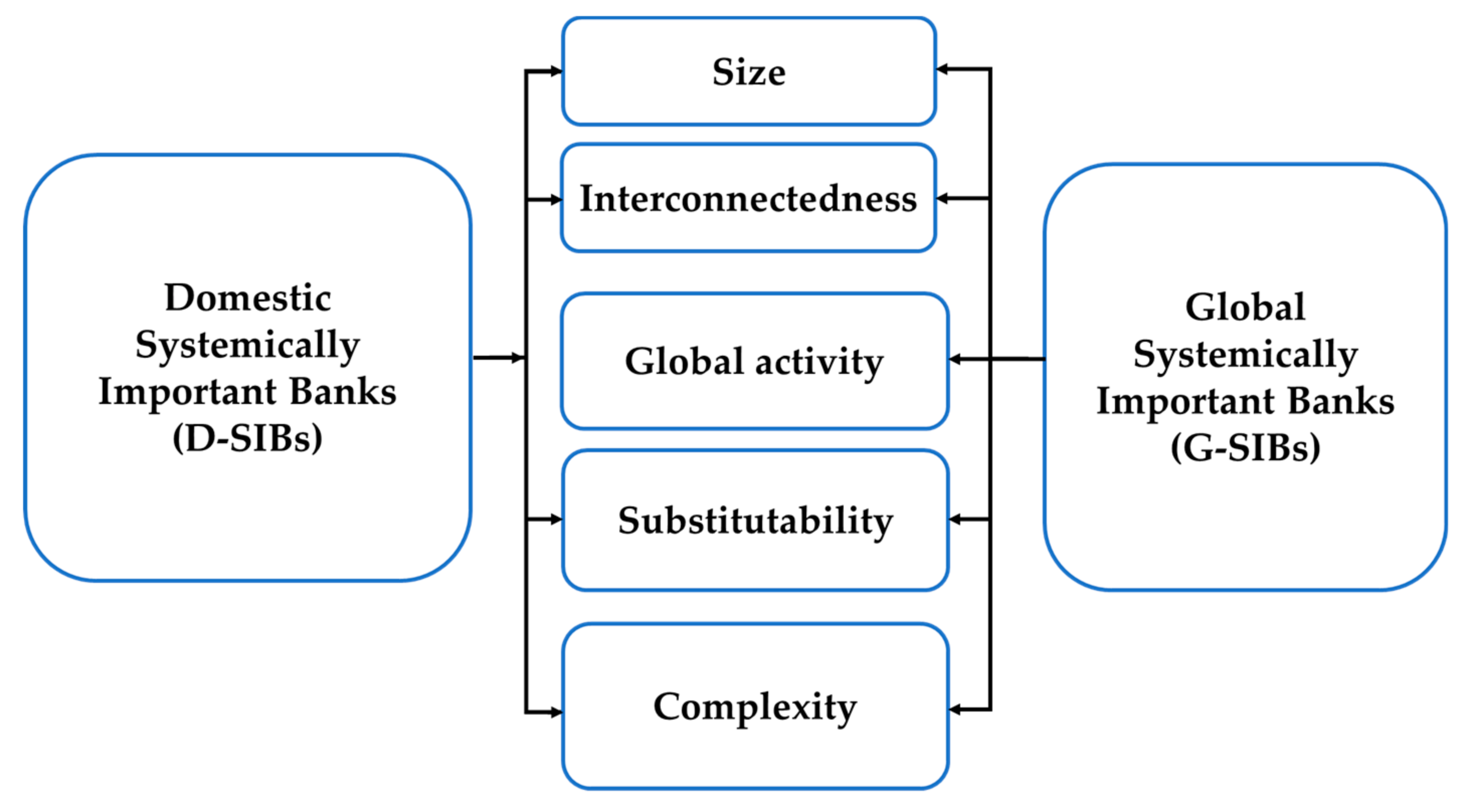
Currently, the systemic risk evaluation approaches for identify the systemic importance of the SIFIs, could be divided into two categories: the indicator approach and the market-based approach. The indicator approach is built based on judgment from experience, which assesses the systemic importance of a financial institution from different perspectives [18]. 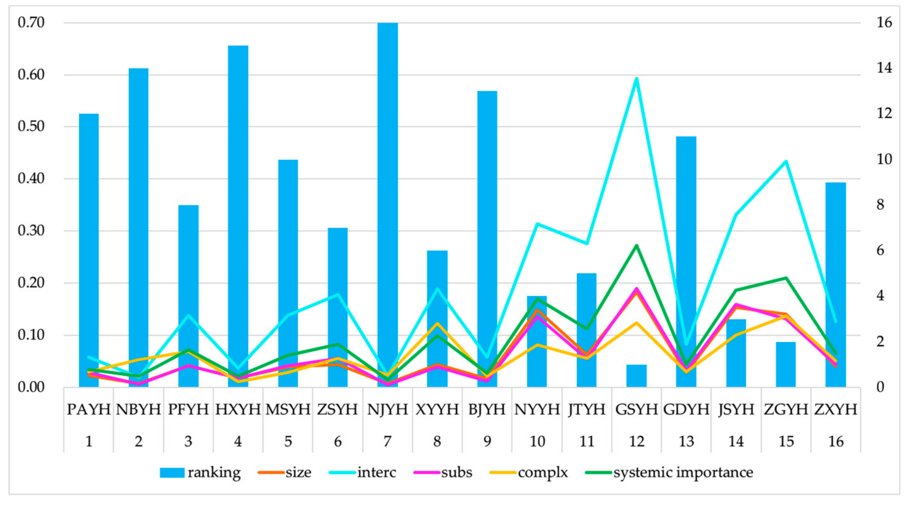Based on the report of the Basel Committee on Banking Supervision (BCBS) [19,20], we illustrate the indicator system with Figure 1, which contains the main indicators used to access systemically important global and domestic banks. This system comprises four or five major categories of indicators, and each major category consists of several subindicators. When measuring the systemic importance of a bank, we first calculate each subindicator and derive the index of each major category with equal weight, and then we obtain the systemic importance index with equal weight.

In comparison with the indicator approach, the market-based approach directly measures the contribution of a financial institution to the whole financial system based on daily or quarterly data derived from financial markets, and identifies the systemically important financial institutions via the quantitative results. This method can capture more characteristics of financial institutions based on the market data than the traditional indicator approach. We will discuss the difference of the results based on the indicator approach and the market-based CoVaR model in Section 3.3.

The core model in this paper, “CoVaR”, is an abbreviation for “Conditional Value at Risk”, which has been increasingly applied in the field of systemic risk and can be used for analyzing the systemic risk in different perspectives. The idea of CoVaR was first proposed by Adrian and Brunnermeier [21]. This model has experienced several years of development and was published in the 12th issue of American Economic Review in 2016. The basic concept and methodology of the CoVaR were originally built based on Value at Risk (VaR), which measures the maximum loss of a financial institution at a certain confidence level. The prefix of CoVaR, namely “Co”, shows that “VaR” is conditional. CoVaR is defined as the VaR of the financial system conditional on a financial institution, while ΔCoVaR refers to the difference between the CoVaR when the institution is in distress and the CoVaR when the institution is in a normal state, which captures the contribution of the institution to the systemic risk of the financial system [22].

The CoVaR model, a market-based approach, is chosen as the core model for the following reasons. First, the traditional supervision focuses on the individual risks of financial institutions using risk indicators, including VaR, but it does not consider the risk at a system-wide level, especially the spillover effect of an institution to the system. CoVaR can efficiently measure the contributions of the institution to the systemic risk. As Adrian and Brunnermeier [22] pointed out, there are two situations in the banking industry: (1) There are some large banks in the banking system, and these banks are highly interconnected. When they are in distress, the risks transfer to the other banks, and cause a system-wide effect in the industry. (2) There are some small banks, but they may cause a herd effect and possibly engender a crisis. The spillover effect of a bank on systemic risk can be modeled with CoVaR. Second, the CoVaR model can measure the contribution to the system when a financial institution is in distress and in a normal state. It can also evaluate the exposure of an institution when the system is in distress (i.e., when a crisis breaks out). Third, we apply the CoVaR model based on data from the financial markets and can capture the changes in systemic risk contributions dynamically.

As the CoVaR model is built based on data from financial markets, it has been applied in an increasing number of studies, domestically and internationally. Drakos and Kouretas measured the contribution of listed financial institutions to systemic risk based on the daily data of the United Kingdom (UK) and the United States (US) financial institutions from 2000 to 2012. Based on the data, the authors found that all financial institutions had increased their contributions to systemic risk in the wake of the global financial crisis. In addition, for UK, banks contributed the most to the systemic risk; for US, the financial institutions that contributed the most to the systemic risk were US domestic banks [23]. Deng measured the risk spillover effects of financial institutions by using the CoVaR model based on quarterly data. Deng’s study suggested that during the sample period of 2010–2017, when the banking industry was in distress, the spillover effect on the whole financial market was stronger than those of the other types of the financial institutions. The study also measured the spillover effect when other financial industry is in distress. The results showed that the Chinese banking industry could withstand external shocks from other financial industries well, and the value of the risk spillover effect was not high [24]. Using the CoVaR model, Wang et al. used 14 banks as a sample. The research showed that the sizes of HXYH and XYYH were not large compared to the state-owned banks in China (in this paper, we denote the banks by the acronyms of the Chinese pinyin names for brevity). Meanwhile, the results showed that the risk spillover effects of these two banks on the Chinese banking system are even higher than those of the state-owned banks, including ZGYH and GSYH [25]. Verma et al. built a CoVaR model to analyze the Indian banking industry. Their study was based on the weekly frequency data of Indian banks, including state-owned banks and private banks, and they found that the state-owned banks were more stable in the times of crisis than private banks [26]. Girardi and Ergün analyzed the systemic risk contributions of 74 financial institutions during the sample period from 2000 to 2008 with a dynamic CoVaR model. They found that depository institutions contributed more to the systemic risk than other financial institutions. Moreover, they observed a positive and statistically significant effect of size on ΔCoVaR [27]. López-Espinosa et al. measured the systemic risk contributions of international large banks with the data spanning from 2001 to 2009, and the results showed that the average systemic risk contributions is higher in the crisis times than those in the pre-crisis times [28]. In addition, CoVaR can also be used in the related areas (e.g., the spillover effect in the debt market). Zheng et al. [29] found that since 2006, the liquidity risk indicators of big banks including ZGYH, JSYH, GSYH and JTYH had been relatively stable. The risk indicators of the joint-stock banks were highest, while the fluctuations of the risk indicators of the city commercial banks were also high. They used the CoVaR model to analyze the spillover effect of the liquidity risk of banks with the quarterly data of 14 banks derived from financial reports. The results showed that the joint-stock banks contributed the most to the risks of the whole banking system. The authors believed that for the joint-stock banks, their motivations to pursue profit are stronger than those of the other banks, and they are thus more active in the interbank market, thereby contributing more risk. Reboredo and Ugolini modeled the systemic risk of the European sovereign debt markets during the period of 2000–2012 with the CoVaR model. They found that there was a similar trend of the systemic risk across all debt markets [30]. Bernal et al. pointed out that ΔCoVaR is a useful method, which assesses the effect of the financial distress of a single financial institution. They applied the method in measuring the spillover effect of the bond market in a country to the Eurozone bond market [31].

We contribute to the existing studies in several perspectives. First, in this paper, based on the daily data derived from financial markets, we build a series of CoVaR models and calculate the CoVaR when the sample banks are in a normal state or in distress. On this basis, we derive their contributions to systemic risk, namely ΔCoVaR. Typically, the papers related to systemic risk measurement using CoVaR focus on an overall analysis of the banks during the sample period. We introduce a year-by-year analysis, which can capture the dynamic changes of systemic risks and the rankings of systemic importance. Second, for the first time, we jointly build static CoVaR, dynamic CoVaR, and Exposure CoVaR models for analyzing China’s listed banks. The contributions can be subdivided into three parts: (1) Based on the daily data derived from the financial markets, the traditional static CoVaR model is constructed to measure the systemic risk contribution (ΔCoVaR) of the sample banks with the combination of a year-by-year analysis and an overall analysis. (2) Considering the “time-varying” characteristics of the returns of the banking system and banks, seven kinds of state variables are introduced to establish a dynamic CoVaR model. (3) On the basis of the dynamic CoVaR model, the role of the return series of the banking system and those of a bank in the model are reversed, and the Exposure CoVaR model is established to calculate the risk exposure of a single bank when the whole banking system is unstable. Third, we also consider the extreme circumstance that a bank faces by using a 1% quantile. This further enrich the analysis of China’s banks’ systemic risk contribution. Fourth, we take the effects of Fintech and non-bank financial institutions into considerations, and modify the base model. Fifth, we conduct the indicator approach, and analyze the results based on the indicator approach and the CoVaR models by introducing Spearman’s rank correlation. The results of statistical tests enrich the existing studies. We provide possible explanations and suggestions for improving financial supervision and maintaining financial stability.

The rest of the paper is structured as follows. In Section 2, we present the market-based systemic risk estimation methodologies including the static, dynamic, and exposure CoVaR models, and make an introduction of the sample. In Section 3, we first model the contribution of each bank to the systemic risk with the static CoVaR model. Then, we introduce the state variables, and the estimation process becomes more dynamic with the dynamic CoVaR model. Furthermore, we extend the research with a series of models aiming at measuring the systemic risk contribution when a bank is in extreme circumstance, another type of the systemic risk (the bank exposure), and the contribution to systemic risk which considers the effects of Fintech and non-bank financial institutions. We also analyze the differences of the results based on the indicator approach and the CoVaR approach. Section 4 concludes the paper.

2. Materials and Methods

2.1. Static CoVaR Model

The traditional static CoVaR model (hereinafter we also use “static model”) is built based on the concept of VaR. According to Adrian and Brunnermeier [22], the VaR of bank i can be defined as follow. In other words, VaR is defined as the $q$th quantile of the conditional probability distribution.

$$Pr\left(X^i\le Va{R}_q^i\right)=q\%$$

(1)

The CoVaR of the financial system represents the maximum loss it experiences when bank i faces events, namely $E\left(X^i\right)$. Recalling Equation (1), we can define the CoVaR as follow. Furthermore, if the bank is in distress, $q$ = 5; if the bank is in a normal state, $q$ = 50.

$$Pr\left(X^{bank}|E\left(X^i\right)\le CoVa{R}_q^{bank|E\left(X^i\right)}\right)=q\%$$

(2)

where i and bank refer to bank i and the whole banking system. The stock prices and stock index series are treated with natural logarithmic transformation. $X^i$ is a series of the returns of the stock prices of bank i. $X^{bank}$ is a series of the returns of the banking system index, and the index is constructed by the average of the stock prices of the sample banks weighted by their lagged market values.

In Equation (3), ΔCoVaR is defined by the difference between the two CoVaRs: the one under distress and the one in a normal state. ΔCoVaR reflects the contribution of a bank to systemic risk, and the more a bank contributes, the more important the bank is in the banking system. In other words, the ranking of a bank in terms of its ΔCoVaR can be considered as a ranking of systemic importance.

$$\Delta CoVa{R}_q^{bank|i}=CoVa{R}_q^{bank|X^i=Va{R}_5^i}-CoVa{R}_q^{bank|X^i=Va{R}_{median}^i}$$

(3)

Based on [22], to estimate ΔCoVaR, we need to build a quantile regression model with two variables ($X^i$ and $X^{bank}$) and use a 5% quantile, as shown in Equation (4). $\alpha$, $\beta$, and $\epsilon$ are used to denote the intercept, coefficient, and stochastic disturbance of the regression, respectively. Second, we predict $X^{bank}$ with a $X^i$ of $Va{R}_q^i$ and let $q$ = 5 and $q$ = 50. Then, we derive the two CoVaRs in Equation (3) and calculate ΔCoVaR.

$$X^{bank|X^i}={\alpha }_q^i+{\beta }_q^i{X}^i+{\epsilon }_q^i$$

(4)

In this paper, for simplicity, we use the acronyms of the sample banks’ Chinese pinyin names as their abbreviations. In addition, as CoVaR and ΔCoVaR are two important elements in the following models, we simply use “static CoVaR model” and “dynamic CoVaR model” in the following sections. Furthermore, when we discuss the results, we use “CoVaR” or “ΔCoVaR” to analyze the sample banks more precisely. In a year-by-year analysis, the data on the specific year are used for computation and we use all the data for measurement in the overall analysis. Because the CoVaR of a bank in distress and ΔCoVaR are small and not positive, we use their absolute values and magnify the values 1000 times in the following charts of all CoVaR models for better comparison and illustration. In addition, all results of CoVaRs and ΔCoVaRs are rounded to two decimal places.

2.2. Dynamic CoVaR Model

The dynamic CoVaR model (hereinafter we also use “dynamic model”) is built based on the static CoVaR model. As Scaillet [32] pointed out, an appropriate model for measuring risk should consider the time-varying market conditions. By introducing a series of lagged state variables, $X^i$ and $X^{bank}$ are considered as the functions of the state variables (namely $StateVar{s}_{t-1}$) and become time-varying. Namely, the two variables change with the state variables. Thus, the time-varying characteristics can be captured and the suffix “t” is added to $X^i$ and $X^{bank}$. According to [22], the calculation procedures can be summarized as follows.

First, we use quantile regression to analyze the relationship between the state variables and the bank stock returns (see Equation (5)). $\alpha$, $\omega$, and $\epsilon$ respectively denote the intercept, coefficient, and stochastic disturbance. Let the quantile be 5% and 50%, we then derive the VaRs for a bank in distress and in a normal state, respectively.

$$X_t^i={\alpha }_q^{\mathrm{i}}+{\omega }_q^{\mathrm{i}}StateVar{s}_{t-1}+{\epsilon }_{q,t}^i$$

(5)

Second, we introduce the state variables into Equation (4) and modify the equation (see Equation (6)). Hereinafter, since the denotations of the intercept and the other terms of the regression are similar to those in Equations (4) and (5), which are easy to understand, the introduction of the denotations is omitted for brevity. Following the similar procedure used in the static CoVaR model, we derive the CoVaRs that are in two states based on Equation (6):

$$X_t^{bank|X^i}={\alpha }_q^{\mathrm{i}}+{\mu }_q^{\mathrm{i}}{X}_t^i+{\theta }_q^{\mathrm{i}}StateVar{s}_{t-1}+{\epsilon }_{q,t}^i$$

(6)

Third, ΔCoVaR is defined as the difference between two CoVaRs that contain the same parts including the terms of the intercept and state variables. Therefore, the calculation of ΔCoVaR can be further simplified as the product of the coefficient of regression and the difference between two VaRs.

As Adrian and Brunnermeier [21,22] suggested, the selection of state variables should be liquid and tractable. They should also accurately capture the time-varying characteristics of the returns in different states. On this basis, we consider both the data availability of the related indicators in China and the corresponding studies (see [33,34,35,36]). Then, the state variables system is constructed with variables from seven perspectives, as shown in

Table 3. The system of the state variables that used in the dynamic CoVaR ¹ model.

No.	State Variable	Definition
1	Interest rate risk	The change in the 6-month government bond yield.
2	Term structure	The change in the credit spread between the 10-year government bond yield and 6-month government bond yield.
3	Credit spread	The change in the credit spread between the 10-year AAA-rated corporate bond yield and 10-year government bond yield.
4	Liquidity spread	The difference between the 6-month Shibor (Shanghai Interbank Offered Rate) and the 6-month government bond yield.
5	Real estate stock return	The return of the China Shanghai–Shenzhen 300 real estate stock index.
6	Volatility of the stock market	The 22-day rolling standard deviation of the return of Shanghai–Shenzhen 300 stock index.
7	Return of the stock markets	The return of the Shanghai–Shenzhen 300 stock index.

¹ CoVaR refers to the Conditional Value at Risk.

.

2.3. Exposure CoVaR Model

The Exposure CoVaR model (hereinafter we also use “exposure model”) can be considered as an extension of the dynamic CoVaR model, but with a focus on the maximum loss (i.e., the risk exposure) of a bank when the whole banking system is in a state of financial instability. By changing the role of the banking system and the bank in the dynamic CoVaR model, we can measure the exposure that a bank faces when there is a system-wide risk in the banking industry.

$$X_t^{bank}={\alpha }_q^{bank}+{\omega }_q^{bank}StateVar{s}_{t-1}+{\epsilon }_{q,t}^{bank}$$

(7)

First, using quantile regression, we estimate the parameters in Equation (7) and derive the VaRs in two states (the bank in distress or in a normal state) with the predicted value of the regression. Second, according to the estimation of Equation (8) and the concept of CoVaR, we derive the Exposure CoVaRs based on the two VaRs, and the Exposure ΔCoVaR is the product of the coefficient of regression and the difference between two VaRs:

$$X_t^{i|X^{bank}}={\alpha }_q^{bank}+{\mu }_q^{bank}{X}_t^{bank}+{\theta }_q^{bank}StateVar{s}_{t-1}+{\epsilon }_{q,t}^{bank}$$

(8)

2.4. Sample Description

As the IMF [4] pointed out, the digital economy era starts from 2001. Meanwhile, there were only three commercial banks (PAYH, PFYH, and MSYH) listed in China’s A-share market in 2001. We take a comprehensive consideration of both the number of the sample banks and the development of the digital economy. The sample period starts from 2011, which covers the entire period of the 12th Five-Year Plan (2011–2015) for the economic and social development of the People’s Republic of China, as well as a part of the period of the 13th Five-Year Plan (2016–2020). According to the 12th Five-Year Plan, Chinese government planned to improve the level of informatization. During the period, the digital economy grew rapidly with the transformation of traditional banking activities and the appearance of Fintech. Based on the data released by the National Bureau of Statistics of China (NBSC) [37], the level of the development of the digital economy in China, which can be measured by the number of the broad band subscribers of the Internet, increased from 150.001 million in 2011 to 407.382 million in 2018. Besides, the international internet bandwidth grew from 1389.529 thousand million bits per second (Mbps) in 2011 to 8946.570 thousand Mbps in 2018. As the collection of data was finished by the end of 2018, the sample period was chosen as 2011–2018. Moreover, there were 28 listed banks by the end of 2018. Among them, 16 banks had a sufficient quantity of data for the sample period. Therefore, they were chosen as the sample.

Table 4. The fundamental information of 16 sample banks.

ID	Stock Code	Abbr	SE	Type	IPO Date	Number of Employees	Total Assets
1	000001	PAYH	SZ	A2	1991/4/3	34626	3418.59
2	002142	NBYH	SZ	A3	2007/7/19	13684	1116.42
3	600000	PFYH	SH	A2	1999/11/10	55692	6289.61
4	600015	HXYH	SH	A2	2003/9/12	41283	2680.58
5	600016	MSYH	SH	A2	2000/12/19	58338	5994.82
6	600036	ZSYH	SH	A2	2002/4/9	74590	6745.73
7	601009	NJYH	SH	A3	2007/7/19	10721	1243.27
8	601166	XYYH	SH	A2	2007/2/5	63044	6711.66
9	601169	BJYH	SH	A3	2007/9/19	14760	2572.87
10	601288	NYYH	SH	A1	2010/7/15	473691	22609.47
11	601328	JTYH	SH	A1	2007/5/15	89542	9531.17
12	601398	GSYH	SH	A1	2006/10/27	449296	27699.54
13	601818	GDYH	SH	A2	2010/8/18	44982	4357.33
14	601939	JSYH	SH	A1	2007/9/25	345971	23222.69
15	601988	ZGYH	SH	A1	2006/7/5	310119	21267.28
16	601998	ZXYH	SH	A2	2007/4/27	56415	6066.71

¹ The “Abbr” refers to the acronyms of a bank’s Chinese pinyin names; the “SE” refers to the stock exchange where a bank is listed, moreover, “SZ” and “SH” refer to the Shenzhen Stock Exchange and the Shanghai Stock Exchange, respectively. the “Type” refers to the ownership type of a bank, moreover, “A1”, “A2”, and “A3” respectively refer to state-owned commercial banks (SOE banks), joint-stock commercial banks (JOI banks), and city commercial banks (CCB banks); the “IPO Date” refers to the date of the initial public offering (IPO) of a bank; the unit for the total assets is 100 million Chinese yuan.

contains the fundamental information of the banks. According to the public-disclosed statistical data released by the CBIRC, by the end of the fourth quarter of 2018, the total assets of commercial banks in China reached 209.9638 trillion yuan. As seen in Table 4, the total assets of the sample banks reached 151.5277 trillion yuan, which comprised a large proportion (72.17%) of the banking industry. Therefore, this sample is very representative.

3. Results

3.1. System Risk Contribution of a Bank (Static Model)

3.1.1. Year-by-Year Analysis

Figure 2A shows the measurements of the CoVaR and ΔCoVaR of the listed banks in 2011. For a list of the banks corresponding to all abbreviations, see Table 4. From the perspective of CoVaR, when the bank is in distress (in other words, when the stock return of the bank lies in the 5% quantile), the loss of the banking system when NJYH is in distress, is highest, with the value of CoVaR reaching 25.15. The CoVaRs of XYYH, ZSYH, PAYH, and BJYH are also higher than those of the other banks, and both their values exceed 24. All the banks are CCB banks or JOI banks. In terms of SOE banks, the CoVaR of GSYH ranks 1st, with a value of 23.88, and it ranks 6th among the sample banks. In addition, the CoVaRs of the other SOE banks (including NYYH, JTYH, ZGYH, and JSYH) are, respectively, 23.17, 22.75, 21.15, and 20.91, with the rankings of 8, 12, 15, and 16.

From the perspective of ΔCoVaR, the ΔCoVaR of ZSYH ranks 1st, with a value of 16.75. The ΔCoVaRs of XYYH, NJYH, BJYH, JTYH, PFYH, and GDYH are relatively high in the industry, with values of 16.24, 16.20, 15.79, 15.58, and 15.37. We find that, there is only one SOE bank among the seven banks, while the other banks are JOI or CCB banks. Therefore, the results of CoVaR and ΔCoVaR show that the maximum loss of the financial system when each SOE bank is in distress is not higher than that of some JOI and CCB banks; moreover, the contribution of a SOE bank to systemic risk is not bigger than those of JOI and CCB banks.

According to Figure 2B, the industrial averages of the CoVaRs and ΔCoVaRs of the sample banks in 2012 are lower than those in 2011. The CoVaR of GDYH ranks 1st (19.10). Further, the CoVaRs of ZXYH, JSYH, HXYH, MSYH, NJYH, XYYH, and JTYH rank in the top 50% in the industry. From the perspective of ΔCoVaR, GDYH also ranks 1st (12.10). The ΔCoVaRs of JSYH, ZXYH, HXYH, GSYH, JTYH, and XYYH rank from 2nd to 7th. Therefore, the relative rankings of the systemic risk contributions of the three SOE banks (including JSYH, GSYH, and JTYH) increase, while the rankings of the other SOE banks (including ZGYH and NYYH) do not change greatly, and their systemic contributions are relatively lower in the industry, with values of 7.84 and 8.70. In 2012, eight banks belonged to the group whose ΔCoVaR values are lower than 10: ZSYH (9.92), MSYH (9.63), PFYH (8.87), NYYH (8.70), ZGYH (7.84), NBYH (7.80), BJYH (7.48), and PAYH (6.61). The contributions of these banks are small. Moreover, the ΔCoVaR of PAYH in 2012 is the lowest during the period of 2011–2015.

Figure 3A shows that the average CoVaR and ΔCoVaR for the sample banks in 2013 are higher than those in 2012. The CoVaR of XYYH ranks the lowest in 2013, with a value of 25.81. Meanwhile, it is 135.16% of the CoVaR of GDYH (19.10), which ranks the highest for 2012. The CoVaRs of GSYH, JTYH, ZGYH, HXYH, and NJYH are high levels in the industry, with values of 32.73, 32.55, 32.04, 31.89, 31.54, and 31.48. This indicates that when three (including GSYH, JTYH and ZGYH) of the “Big Five Banks” (including GSYH, JSYH, NYYH, ZGYH and JTYH) in China are in distress, the banking system faces higher losses compared to situations when the other banks are in distress. In terms of contributions to systemic risk, JTYH ranks 1st, with a ΔCoVaR of 21.10, indicating that JTYH contributes the most to systemic risk. HXYH, BJYH, MSYH, ZGYH, and NJYH contribute the next most to systemic risk; the values of their ΔCoVaRs both exceed 18, ranging from 18.10 to 20.02.

According to Figure 3B, compared to the results for 2013, there are only relatively small changes in terms of the CoVaR and ΔCoVaR for 2014. Meanwhile, the CoVaR rankings change, and HXYH, PAYH, BJYH, NBYH, XYYH, and ZXYH, respectively, rank from 1st to 6th, with values of 27.50, 25.88, 25.09, 24.90, and 24.43. In 2013, three SOE banks, GSYH, JTYH, and ZGYH rank from 1st to 3rd. However, their rankings, respectively, changed to 8th, 16th, and 7th, with values of 23.19, 21.00, and 23.56. From the perspective of systemic risk contributions, PAYH ranks 1st with a ΔCoVaR of 16.97. Next come PFYH, HXYH, XYYH, NBYH, GSYH, ZSYH, and ZGYH, whose ΔCoVaR values range from 13.96 to 16.21. ZXYH contributes the least to systemic risk, with a ΔCoVaR of 8.68, which is the lowest value during the past two years.

As shown in Figure 4A, in 2015, both the CoVaRs and ΔCoVaRs of the listed banks change greatly. There are 11 banks whose CoVaR is higher than 50, which occupies a proportion of 68.75% of the sample. BJYH ranks 1st, with a CoVaR of 55.39. Next come MSYH, HXYH, NBYH, PFYH, ZGYH, XYYH, ZXYH, NJYH, PAYH and NYYH, which rank from 2nd to 11th, with CoVaRs of 55.23, 54.92, 54.66, 53.55, 52.13, 51.68, 51.37, 50.56, 50.43, and 50.32, respectively. JTYH, GDYH, and GSYH rank from 12th to 14th, with CoVaRs of 49.98, 48.85, and 48.70. Both JSYH and ZSYH rank 15th, with CoVaRs of 47.41. Because of the stock market crash in 2015, even the lowest value CoVaR is higher than the historical highest value. For instance, GSYH ranks 1st with a CoVaR of 32.73 and ranks 15th in 2015 with a CoVaR of 48.70, which is an increase of nearly 50%. Moreover, the highest CoVaR (BJYH, 55.39) and the lowest CoVaR (JSYH and ZSYH, 47.41) in the banking industry in 2015 are 1.69 and 1.45 times the highest CoVaR (GSYH in 2013, 32.73) during the period of 2011–2014.

In terms of the systemic risk contributions measured by ΔCoVaRs, HXYH ranks highest, with a value of 37.53 in 2015. There are 11 banks whose ΔCoVaRs are higher than 30, accounting for 68.75% of the total sample banks. XYYH, NYYH, JSYH, PAYH, ZGYH, NBYH, MSYH, GDYH, and PFYH rank from 2nd to 11th, and their values in 2015, respectively, are 35.50, 35.48, 35.36, 34.14, 33.52, 31.62, 31.47, 31.45, 30.88, and 30.57, which are higher than that the historical highest value during the period of 2011–2014. BJYH, GSYH, NJYH, ZXYH, and ZSYH rank from 12th to 16th, with ΔCoVaRs of 28.84, 28.73, 28.38, 27.22, and 26.94. The ΔCoVaRs of all the samples exceed 25.0. Even the lowest ΔCoVaR (ZSYH, 26.94) in 2015 is 1.28 times the historical highest value (JTYH in 2013, 21.10), and the highest ΔCoVaR (HXYH, 37.53) in 2015 is 1.78 times that in 2013. Furthermore, the lowest ΔCoVaR (ZSYH, 26.94) is 4.07 times the historical lowest ΔCoVaR (PAYH in 2012, 6.61).

In 2015, the CoVaRs and ΔCoVaRs of the listed banks face severe fluctuations, and the averages of the values increase greatly in comparison with the measurements in 2014. According to Figure 4B, the overall levels of the CoVaRs and ΔCoVaRs decrease in 2016, which is similar to the results in 2014. The CoVaRs range from 17.17 to 26.45. BJYH ranks 1st, with a CoVaR of 26.45. The CoVaRs of 14 banks are higher than 20, which accounts for 87.5% of the total sample. The values range from 20.01 to 26.45. Next come MSYH, ZSYH, GSYH, NYYH, NJYH, NBYH, PFYH, XYYH, ZXYH, GDYH, JSYH, ZGYH, and HXYH, which rank from 2nd to 14th. Note that BJYH and MSYH, a CCB bank and a JOI bank, respectively, rank 1st and 2nd in both 2015 and 2016.

As seen from Figure 5A, in 2017, the CoVaRs and ΔCoVaRs of all the banks decrease by a certain degree, except for the CoVaR of JTYH, which increased by 5.42%. Overall, if a sample bank is in distress, the VaR of the banking system decreases. From the perspective of the CoVaR rankings, NYYH, NJYH, GDYH, XYYH, and GSYH rank from 1st to 5th, indicating that the maximum loss of the banking industry is relatively high when the banks are in distress. According to the ΔCoVaR rankings, five banks rank from 1st to 5th, including three SOE banks (GSYH, NYYH, and JSYH) and two joint-stock banks (XYYH and GDYH). When these banks are in distress, their contributions to systemic risk are relatively high in the industry. For instance, XYYH ranks 1st for CoVaR, and its CoVaR (11.12) is 2.07 times that of PFYH, which has the lowest CoVaR (5.37).

According to Figure 5B, overall, the CoVaRs and ΔCoVaRs of the sample banks increased in 2018. XYYH ranks the lowest for CoVaR and ΔCoVaR, while its indicators are higher than those in 2017, indicating an increase in risk. In terms of CoVaRs, four CCB banks, including ZXYH, PFYH, ZSYH, and MSYH, rank 1st, 2nd, 4th, and 6th; two CCB banks, including NJYH and BJYH, rank 3rd and 4th. The five SOE banks, including JTYH, JSYH, NYYH, ZGYH, and GSYH, rank 7th, 9th, 10th, 13th, and 15th. In terms of ΔCoVaRs, three SOE banks (JSYH, NYYH, and ZGYH) and four JOI banks (ZSYH, ZXYH, PAYH, and PFYH) are top seven banks. ZSYH, JSYH, NYYH, ZXYH, PAYH, ZGYH, and PFYH, respectively, rank from 1st to 7th.

3.1.2. Overall Analysis

Figure 6 shows the calculations of CoVaRs and ΔCoVaRs of the sample banks during the entire sample period. On the whole, JOI banks and CCB banks are in the top 50% of the sample banks in terms of CoVaRs. PFYH, a JOI bank, with a CoVaR exceeding 30, ranks 1st in the listed banking industry. Among the CCB banks, NJYH ranks 1st in the subindustry and ranks 2nd in the banking industry. Both the CoVaRs of NBYH and BJYH exceed 28 and, respectively, rank 5th and 8th. Among the JOI banks, ZXYH and GDYH rank 12th and 15th, with CoVaRs of 27.16 and 26.04. The CoVaRs of the SOE banks are lower than those of the CCB banks and JOI banks, except for ZXYH and GDYH. GSYH and NYYH rank 10th and 11th, with the CoVaRs of 27.98 and 27.80. JSYH, ZGYH, and JTYH rank 13th, 14th, and 16th, with CoVaRs of 26.25, 26.18, and 25.84.

In terms of ΔCoVaRs, three SOE banks (GSYH, NYYH, and JSYH) and five JOI banks (ZSYH, HXYH, PFYH, XYYH, and MSYH) rank in the top 50% of the sample banks during the sample period. Three CCB banks (NBYH, NJYH, and BJYH) rank from 9th to 11th. Among the SOE banks, GSYH, NYYH, and JSYH rank 3rd, 5th, and 7th; their contributions to systemic risk are at middle or upper middle levels. The ΔCoVaR rankings of JTYH and ZGYH are only 13 and 15, indicating that their contributions to systemic risk are relatively low in the industry. Among the JOI banks, ZSYH and HXYH contribute the most to systemic risk and rank 1st and 2nd in the industry. Meanwhile, the JOI banks GDYH and ZXYH, respectively, rank 14th and 16th.

According to the year-by-year analysis and overall analysis, we find that the levels of risk measured by CoVaR and ΔCoVaR vary across different time periods due to the changes in domestic and international economic and financial situations. Particularly, the risk levels significantly increase during certain time periods. For instance, the “money shortage” happened in 2013, the “stock market crash” occurred in 2015, and Sino–US trade war broke out in 2018. Moreover, we find that the CoVaR and ΔCoVaR rankings of most listed banks changed dynamically.

3.2. System Risk Contribution of a Bank (Dynamic Model)

3.2.1. Year-by-Year Analysis

In the above section, we measured the risks of sample banks by using CoVaR and ΔCoVaR and analyzed those risks using a year-by-year and overall analysis. In this section, we introduce state variables into the estimation of CoVaR and ΔCoVaR, and the two indicators become time-varying. For simplicity, we pay more attention to the dynamic changes of systemic risk contribution. Therefore, we analyze ΔCoVaR based on the mean and standard deviation (hereinafter we use “Std.” in the figures, measured by the standard deviation of daily ΔCoVaR) in this section. According to Figure 7A, for 2011, there are seven banks that contribute the most to the systemic risk of the banking system based on the means of ΔCoVaR: three JOI banks, two SOE banks, and two CCB banks. These banks are HXYH, XYYH, ZSYH, GSYH, NJYH, NYYH, and BJYH. Among the banks, HXYH ranks 1st, with a ΔCoVaR of 16.55, and that of the other six banks both exceed 15. In terms of the standard deviations of the ΔCoVaRs, the ΔCoVaR fluctuations of the three JOI banks (HXYH, XYYH, and ZSYH) are at the middle level in the industry, ranking 12th, 10th, and 15th, respectively, thereby indicating that their importance to the systemic risk of the banking system is stable. GSYH, NJYH, and NYYH are at an upper-middle level and, respectively, rank 6th, 7th, and 8th. This indicates that systemic importance rankings have a certain degree of fluctuation.

According to the systemic importance rankings based on the dynamic CoVaR model, For SOE banks, GSYH, NYYH, JSYH, JTYH, and ZGYH rank 4th, 6th, 8th, 11th, and 12th in the industry. The top three JOI banks with the highest systemic importance are HXYH, XYYH, and ZSYH, ranking from 1st to 3rd, while the top two CCB banks are NJYH and BJYH.

As Figure 7B shows, in 2012, among the top seven banks with the highest ΔCoVaRs, six banks belong to the group that contributes that most to systemic risk, including HXYH, ZSYH, XYYH, GSYH, NJYH, and NYYH. Additionally, the ranking of BJYH in ΔCoVaR rises, and its contribution to systemic risk enters the top five. Compared with 2011, the mean and standard deviation of the ΔCoVaR for the whole banking industry decreases. We subdivide the banking industry and find that the rankings of five SOE banks in the subindustry are exactly the same as in 2011. Among the JOI banks, 4 out of the 5 banks with the highest ΔCoVaR in 2012 are systemically important in 2011. Among the CCB banks, the two banks with highest systemic importance are the same as those in 2011. Overall, although the rankings of some banks change slightly, the relative levels of the contributions to systemic risk in 2012 remain unchanged in the subindustries, including JOI, SOE, and CCB.

According to Figure 8A, the industrial average mean and standard deviation of systemic risk contributions increase in 2013 compared with the values in 2012. In terms of the rankings of the means of ΔCoVaRs, the top seven banks with the highest systemic importance comprise four JOI banks, two SOE banks, and one CCB bank. HXYH, which ranks 1st in terms of systemic importance, is also 1st in 2011 and 2012. ZSYH and GSYH, respectively, rank 2nd and 3rd. Among the JOI banks, HXYH, ZSYH, XYYH, and PAYH contribute more to systemic risk. Among SOE banks, the systemic importance of GSYH, JSYH, and ZGYH is at the high level in the subindustry. NBYH is the bank with the highest systemic importance in the CCB subindustry.

As seen in Figure 8B, for 2014, in terms of the measurement of ΔCoVaRs, the industrial mean of systemic risk contributions decreases slightly, while the fluctuation of ΔCoVaRs significantly increases, and the standard deviation grows from 3.84 to 6.55. The standard deviations of the ΔCoVaRs of JSYH, GDYH, ZGYH, NYYH, and JTYH achieve values of 8.80, 8.68, 8.49, 7.96, and 7.96, which are higher than or equal to 1.70 times that in 2013. The average ΔCoVaRs of HXYH, ZSYH, GSYH, XYYH, and BJYH, respectively, rank from 1st to 5th, indicating that their contributions to systemic risk are at high levels in the industry.

According to Figure 9A, in 2015, the means of the standard deviations of the ΔCoVaRs for the listed banking industry both significantly increased. Based on the calculations, the means and standard deviations of the ΔCoVaRs, respectively, are 13.38 and 6.55. Meanwhile, the values are 27.15 and 12.28 in 2015, with growth rates of 102.85% and 87.39%. Moreover, four SOE banks (JSYH, ZGYH, NYYH, and JTYH) ranks in the top five of the means of the ΔCoVaRs. In terms of JOI banks, GDYH, HXYH, and XYYH rank 2nd, 7th, and 8th. For CCB banks, NJYH and NBYH rank 6th and 10th. It is worth noting that the levels of the means of all the banks increase significantly compared to levels in the previous year. JSYH achieves the highest average ΔCoVaRs, with a value of 32.28, which is equivalent to 2.45 times the mean in 2014. Additionally, the average ΔCoVaR of ZXYH is at a low level in the industry, with a value of 19.97, but exceeds the highest average ΔCoVaR of HXYH (14.72).

As shown in Figure 9B, for 2016, the industrial average of the ΔCoVaRs significantly decreases, with values of 15.45. The fluctuation decreases slightly, with values of 6.75. The means of the ΔCoVaRs of HXYH, JSYH, GSYH, ZSYH, NBYH, and ZGYH are at high levels in the banking industry, and most of these banks are SOE banks and JOI banks. Furthermore, among SOE banks, JSYH, GSYH, and ZGYH are more systemically important than JTYH and NYYH. Among JOI banks, HXYH, ZSYH, and GDYH are more systemically important the other JOI banks. Among CCB banks, NBYH is the bank with the highest systemic importance.

Figure 10A shows that the fluctuations of the industrial ΔCoVaR continue to decrease, with a value of 2.37; the mean in 2017 is the lowest during the past seven years, and the average of the contributions of the sample banks to systemic risk significantly drops. According to the ranking of means, five JOI banks (HXYH, ZSYH, PAYH, XYYH, and PFYH), respectively, rank 1st, 2nd, 3rd, 5th, and 7th. Three CCB banks (NBYH, BJYH, and NJYH) rank 6th, 8th, and 9th. In terms of SOE banks, GSYH, JSYH, and NYYH, respectively, rank 4th, 10th, and 11th.

According to Figure 10B, in 2018, compared with the previous year, the average ΔCoVaR of the sample banks decreased by 4.10% while the level of fluctuations increases by 24.0%. There are four SOE banks (JSYH, GSYH, ZGYH, and NYYH) and four JOI banks (HXYH, GDYH, XYYH, and ZSYH) that rank among the top eight banks in terms of the means of their ΔCoVaRs. The systemic risk contributions of the CCB banks (NBYH, NJYH) are at a middle level in the industry, ranking 9th and 10th, with values of 16.98 and 16.67, which exceed the historical highest mean of the ΔCoVaRs in 2017.

3.2.2. Overall Analysis

As seen from Figure 11, the dynamic ΔCoVaR shows that seven banks, including three SOE banks and four JOI banks, contribute the most to the systemic risk. These banks are HXYH, XYYH, JSYH, GSYH, ZSYH, NYYH, and GDYH. Among the banks, the mean of the ΔCoVaR of HXYH achieves 17.20, while that of the other banks exceeds 16.00. In terms of the fluctuations of the ΔCoVaRs, MSYH and ZXYH have a low level of ΔCoVaR standard deviations in the industry, with values of 14.81 and 13.00. However, JSYH, GDYH, ZGYH, NYYH, and XYYH are at the upper level in the means of their ΔCoVaRs, with a higher standard deviations than the other banks, reflecting the dynamic changes of their systemic importance.

3.2.3. Comparison: Static and Dynamic Model

In the above sections, we first assessed the systemic importance of the sample banks with a static CoVaR model, and then we introduced the state variables and conducted an analysis based on the dynamic CoVaR model. In the section, we make a comparison of the overall results derived from the static and dynamic CoVaR models during the entire sample period.

Figure 12 shows the rankings of ΔCoVaRs measured by the dynamic and static CoVaR models. We find that among the SOE banks, for GSYH and NYYH, the rankings based on one model are not significantly different from those based on the other model. GSYH and NYYH, respectively, rank 4th and 6th according to the dynamic CoVaR model and rank 3rd and 5th according to the static CoVaR model. JTYH ranks 11th with the dynamic model and 13th with the static model. The systemic importance rankings of JSYH and ZGYH increase by 4 and 6 in the dynamic model compared to the static model, ranking 3rd and 9th. Among the CCB banks, there is not a significant change between the rankings based on the two models. The systemic importance rankings of both NBYH and BJYH improve by 1 to 10 and 12 in the dynamic model, whereas the ranking of NJYH improves by 2 to 8 in the dynamic model. Among the JOI banks, the dynamic model incorporates the effects of state variables. There is no change in the ranking of ZXYH, while the ranking of systemic importance for PAYH decreases; their contributions to systemic risk are thus at low levels. The change in ranking of HXYH is only 1. Moreover, based on the measurements of both the static and dynamic ΔCoVaR models, its systemic risk contribution is at a high level. Further, the systemic importance of PFYH and MSYH significantly decreases in the dynamic model, while that of ZSYH slightly decreases and is one of the top five highest in the banking industry. The systemic importance rankings of XYYH and GDYH significantly increase.

The static ΔCoVaR is derived from the traditional CoVaR model. As seen from the figure, seven banks (ZSYH, HXYH, GSYH, PFYH, NYYH, XYYH, and JSYH) contribute more than the other banks based on the static model, and six banks (HXYH, XYYH, JSYH, GSYH, ZSYH, and NYYH) are still considered to be banks with highest ΔCoVaRs using the dynamic model. Meanwhile, the dynamic ΔCoVaR contains more information as it incorporates a series of state variables and becomes time-varying. In other words, the accurate systemic risk evaluation should be based on a dynamic model, and the static model is considered as an approach to measure systemic risk and identify the systemically important banks quicker.

3.3. Extended Researches

3.3.1. Systemic Risk Contribution of a Bank (Extreme Circumstance)

The systemic risk contribution of a bank is measured by a ΔCoVaR based on quantile regressions. Typically, a 5% quantile is used to define the state in which a bank is in distress (see [17]). In this section, we use a 1% quantile, and model the systemic risk contributions of a bank when it is in an extreme circumstance. Figure 13 shows the year-by-year measurements of ΔCoVaRs using the dynamic model. We find that the systemic risk contributions of all banks when they are in extreme circumstances are higher than those in the state of distress, which we calculate in Section 3.2. Additionally, it is clearly that the ΔCoVaRs of the sample banks in 2015 are higher than that in the other years. Besides, the ΔCoVaR of each bank in 2018 is less than that in 2015, but it is higher than that in the other years. The figure implies that when a bank faces a severe event (e.g., the stock market crash happened in 2015), it contributes more to the banking system. This can be considered as an “amplification effect”, the extreme event happens (the stock market crash, in 2015; the trade war, in 2018), and amplifies the systemic risk contribution; therefore, the banks contribute more than in the peaceful times when no extreme event happens. This shows the necessities of assessing systemic risk contributions and discovering the SIFIs in China’s banking system. Figure 14 clearly shows that the rankings of the banks in terms of ΔCoVaRs change dynamically over time. However, the rankings of HXYH and ZXYH are stable in every year.

According to Figure 15, for all the banks, the ΔCoVaRs in extreme circumstance increase by more than 10, except for ZXYH. Among the top eight banks in terms of ΔCoVaRs, there are four SOE banks including JTYH, NYYH, JSYH, and ZGYH (respectively rank 3rd, 4th, 5th and 6th). Three JOI banks (HXYH, PFYH, and XYYH) rank 2nd, 7th, and 8th. A CCB bank, namely NBYH, ranks 1st.

3.3.2. Another Type of Systemic Risk: Bank Exposures

Figure 16 shows the Exposure ΔCoVaRs (E-ΔCoVaRs) measurements and rankings during the entire sample period. The values of the E-ΔCoVaRs reflect the maximum loss of a bank when the banking system is in distress. As seen from the figure, among the SOE banks, JTYH, JSYH, NYYH, GSYH, and ZGYH, respectively, rank 11th, 12th, 14th, 15th, and 16th. Therefore, the exposures of the SOE banks are at low levels in the banking industry. Among the CCB banks, NBYH and NJYH, respectively, rank 1st and 5th. Among JOI banks, ZXYH, PAYH, HXYH, and XYYH, respectively, rank 2nd, 3rd, 4th, and 6th. To summarize, when the banking system is in distress, the JOI banks and CCB banks except BJYH, are more affected than all the SOE banks. Therefore, the SOE banks show relatively good stability when the banking system is in distress.

3.3.3. Modified Model: Incorporation of the Effects of Fintech and Non-Bank Financial Institutions

In the section, we modify the dynamic model, and the effects of Fintech and non-bank financial institutions (NBFIs) are introduced as the state variables, which are measured by the returns of China Securities Index (CSI) Fintech stock index and the NBFI stock index. The two variables are selected for three reasons. First, Fintech, namely Finance Technology, is the trend of finance, which transforms the business model of traditional financial institutions and brings financial innovations in the digital economy era. Second, the non-bank financial institutions are considered by China’s central bank to play a more and more important role in China’s financial system [38]. Therefore, we should also take the potential effect of NBFIs into consideration. Third, they all meet the requirements of the selection principles of the state variables. As in the discussion section, we need to compare the year-by-year results; thus, the sample period should cover the entire period of each year. Moreover, the Fintech index has been released since July 2014, therefore the systemic risk is measured based on the data from 2015 to 2018. As seen from Figure 17, during the sample period of 2015–2018, among the top eight banks, JSYH, NYYH, GSYH, and ZGYH, four SOE banks, respectively rank 1st, 2nd, 3rd, and 4th. ZSYH, HXYH and XYYH, three JOI banks respectively rank from 5th to 7th. NBYH, a CCB bank, ranks 8th.

3.3.4. The Indicator Approach and the Covar Model: Differences and Possible Reasons

In this section, we conduct a systemic risk evaluation with the indicator approach, and the variable list is shown in

Table 5. The indicators used in the indicator approach.

No.	Indicators	Definition
1	Size	The total assets.
2	Interconnectedness	The intra-financial system assets and liabilities, including the lendings to banks and other financial institutions, the due from placements with banks and other financial institutions, the redemptory monetary capital for sale, the due to placements with banks and other financial institutions, the borrowings from banks and other financial institutions, and the financial assets sold for repurchase.
3	Substitutability	The loans and advances, the fee and commission income, and the deposits from customers.
4	Complexity	The derivative financial assets and the financial assets that are trading or available for sale.

. We take an example of the systemic risk evaluation in 2018. In Figure 18, from the perspective of the indicator approach, five SOE banks (GSYH, ZGYH, JSYH, NYYH, and JTYH) respectively rank from 1st to 5th. The systemic risks of six JOI banks (XYYH, ZSYH, PFYH, ZXYH, MSYH, and GDYH) are at middle levels. The systemic risks of two JOI banks and three CCB banks are at low levels.

However, according to the measurements of the ΔCoVaRs based on the data from financial markets, the large SOE banks do not always have the highest contributions to systemic risk, which is consistent with the conclusions drawn by [39,40]. Furthermore, some JOI banks and even some CCB banks contribute more to the systemic risk of China’s banking industry than the SOE banks, whose sizes are larger than those of the JOI and CCB banks.

We then calculate the Spearman’s rank correlations between the size rankings and a series of systemic risk indicator rankings. In

Table 6. The results of Spearman’s rank correlations.

Spearman’s Rank Correlation	2011	2012	2013	2014	Proportion (%)
R 1 (indicator approach)	0.953	0.977	0.977	0.959	100.000
Test statistics	0.000	0.000	0.000	0.000	/
R (static ΔCoVaR)	−0.371	0.253	−0.138	−0.162	0.000
Test statistics	0.158	0.345	0.610	0.550	/
R (dynamic ΔCoVaR, 5%)	−0.018	−0.221	0.106	−0.079	0.000
Test statistics	0.948	0.412	0.696	0.770	/
R (exposure ΔCoVaR, 5%)	−0.662	−0.682	−0.677	−0.679	100.000
Test statistics	0.005	0.004	0.004	0.004	/
R (dynamic ΔCoVaR, 1%)	−0.312	−0.191	−0.012	−0.124	0.000
Test statistics	0.240	0.478	0.966	0.649	/
R (modified dynamic ΔCoVaR, 5%)	/	/	/	/	0.000
Test statistics	/	/	/	/	/

¹ The “R” represents the ranking of a bank in terms of the systemic importance based on the result derived from the corresponding model.

and

Table 7. The results of Spearman’s rank correlations.

Spearman’s Rank Correlation	2015	2016	2017	2018	Proportion (%)
R 1 (indicator approach)	0.953	0.977	0.974	0.974	100.000
Test statistics	0.000	0.000	0.000	0.000	/
R (static ΔCoVaR)	0.074	0.356	0.524	0.544	50.000
Test statistics	0.787	0.176	0.037	0.029	/
R (dynamic ΔCoVaR, 5%)	0.359	0.238	−0.191	0.447	0.000
Test statistics	0.172	0.374	0.478	0.083	/
R (exposure ΔCoVaR, 5%)	−0.659	−0.653	−0.694	−0.679	100.000
Test statistics	0.006	0.006	0.003	0.004	/
R (dynamic ΔCoVaR, 1%)	−0.082	−0.082	−0.188	−0.079	0.000
Test statistics	0.762	0.762	0.485	0.770	/
R (modified dynamic ΔCoVaR, 5%)	0.482	0.200	0.303	0.491	0.000
Test statistics	0.059	0.458	0.254	0.053	/

¹ The “R” represents the ranking of a bank in terms of the systemic importance based on the result derived from the corresponding model.

, “R” is the abbreviation of “Ranking”. “Test statistic” refers to the statistic of the test whose null hypothesis is the size rankings and the rankings of a systemic risk indicator are independent. If a test statistic is less than the given significance level (5%), the correlation between the two rankings are statistically significant with a 95% level of confidence. The “Proportion” refers to the proportion of the number of the significant correlations to the number of all the correlations.

We find that the correlation between the bank size rankings and the systemic importance rankings derived from the indicator approach are significant at the 5% level. This is because bank size is an important element of the systemic risk indicator measured by the indicator approach, and the other elements are likely to be affected by the bank size. For instance, the deposit and loan of a big bank are usually higher than that of a small bank. In other words, the bank size directly and indirectly affects the systemic risk indicator using the indicator approach.

If the bank size directly determines the systemic importance of a bank, we expect all the correlations in the following tables to be significant. Besides, we are curious about whether the correlations are positive or not. The results based on the market-based approach imply that for China, the bank size is only negatively correlated with the bank exposures, and the correlation is significant at the 5% level. When the banking system is in distress, the maximum loss of a big bank is smaller than that of a small bank, indicating that the big banks are more stable.

Furthermore, we observe a significant positive correlation between the size rankings and the rankings of the static ΔCoVaRs, only in 2017 and 2018. All the correlations between the size rankings and the rankings based on dynamic ΔCoVaRs derived from three dynamic models (a model with a 5% quantile, a model which considers a bank in extreme circumstance and use a 1% quantile, a model which incorporates the effects of Fintech and non-bank financial institutions) are insignificant at the 5% level. Additionally, the correlations are positive in some years and negative in the other years.

The possible reasons are follows. First, in the era of the digital economy, beyond the existing branches, the popularization of the Internet as well as the development of information technologies especially Fintech make it possible for small banks to compete with big banks on the Internet and provide services for customers in China and possibly in other countries. However, the small banks may not have sufficient experiences and measures to forestall the risks arising from Internet banking activities as the big banks do. Therefore, when a small bank is in distress, it could contribute more to the systemic risk than big banks. Second, for the same reason, when the crisis of a small bank occurs, people may believe that the bank is too small to handle the risk. Therefore, these customers may become too “rational” to trust the bank. They may believe that the bank will run out of money when the crisis event occurs, and their wise choice is to draw money from the small bank as soon as possible. The Internet enables people to draw money faster than before, which may accelerate the bank run and increase the systemic risk in the digital economy era. Third, in the era, customers choose diverse online banking services (i.e., financial products) simply by clicking the mouse. Meanwhile, the banking services may not be transparent enough for customers, and some products may be highly risky. In this way, a small bank can increase the systemic risk.

In addition, according to Acharya and Yorulmazer, regulatory institutions have recognized a phenomenon of “too big to fail” in the financial system, which arouses the interests of researchers and regulators to study the effect of big banks on systemic risk. However, in reality, there may be a situation of “too many to fail” as well, which should be also noticed. They point out that, a small bank may invest in the same direction as a big bank, thus increasing the correlation of investments between banks. Moreover, many small banks have incentives to do so. In this way, the risks at the individual bank level may turn into system-wide risks. In this case, small banks may also induce the systemic risk [41]. Varotto and Zhao propose another way in which a small bank may cause systemic risk: the small bank may occupy a considerable proportion of the banking industry of a certain region [42]. This situation is similar to that of the CCB banks studied in this paper. When people learn that local small banks have gone bankrupt, people may worry that other local banks will also go bankrupt. The bankruptcy of local small banks may be even perceived to herald a national bank crisis or trigger a chain reaction in the banking system. Therefore, we believe that the reform and development of financial supervision should keep pace with the times and be improved by market-based systemic risk estimation methodologies.

Currently, increasingly more empirical studies concentrate on systemic risk and suggest the significance of the effect of small banks on systemic risk. Manguzvane and Muteba [43] applied CoVaR methodology to model the systemic risk of the banking industry in South Africa. The results showed that since the global financial crisis, there had been a huge fluctuation in the ΔCoVaRs of the sample banks. For the means of ΔCoVaR during the sample period, First Rand was the bank with the highest ΔCoVaR, indicating that it is the bank with the most systemic importance to the banking industry in North Africa. Besides, the systemic risk of the African bank’s contribution is the smallest, with a value of ΔCoVaR close to zero. Clearly, the contributions of different banks to systemic risk vary, and supervision should thus be differentiated. Additionally, the authors also find that a small bank in North Africa, namely Capitec, can affect systemic risk as big banks do. Moreover, they observe a noticeable increase of the contribution of Capitec to the systemic risk in the crisis times. Therefore, on the basis of microprudential supervision, which focuses on the individual risk of a financial institution, regulatory institutions should also consider the influence of small banks on systemic risk and adopt the concept of macroprudential supervision. Another study [44] measured systemic risk by the value of ΔCoVaR and found that CCB banks contributed more than SOE banks. The authors thought that, this may be because both SOE banks and CCB banks are backed by government credit, but state credit is higher than that of the local government. Therefore, the market will generate expectations that the state will bail out SOE banks (because they are backed by state credit), making them unlikely to trigger a run after a crisis or affect the stability of the entire banking system. However, JOI banks are not backed by state credit and are not as widely distributed as CCB banks and SOE banks. Therefore, JOI banks contribute more to systemic risk than SOE banks, so size is not the only factor that affects systemic risk contributions. Our research could provide empirical evidence to enrich existing studies from another perspective. The results based on the Exposure CoVaR model indicate that during the sample period, when the banking system is in distress, all the JOI banks and most of the CCB banks are more affected than all the SOE banks, which are less affected. In other words, when the banking industry is in distress, the SOE banks are more stable in the banking industry.

4. Discussion

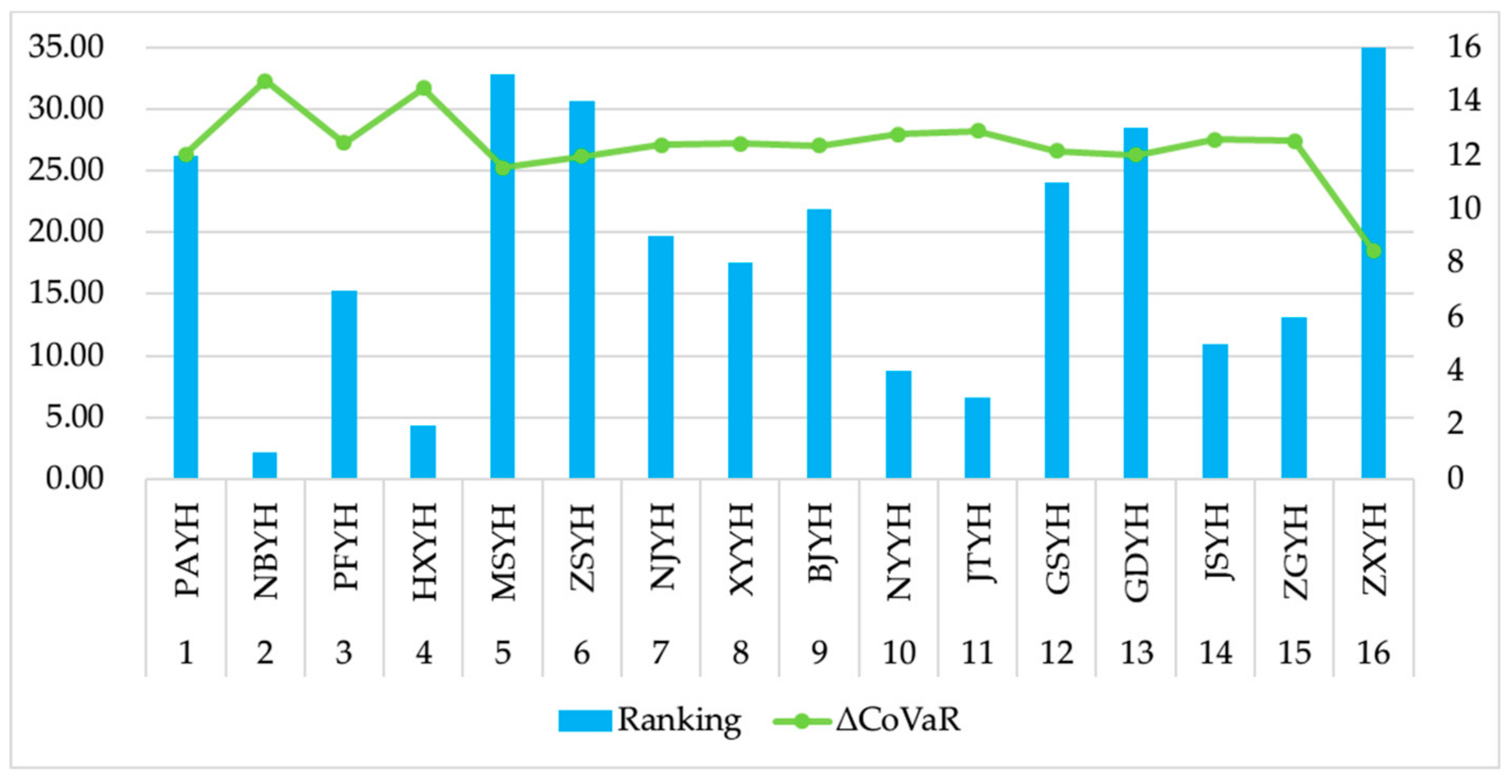
In this paper, we first note that China is a bank-based country and that it is of great significance to study the systemic risks of Chinese banks in the digital economy era. In this paper, based on the static, dynamic, and modified CoVaR models, we quantitatively measure the systemic risk of 16 China’s listed commercial banks during the period of 2011–2018. Our findings and suggestions are as follows.

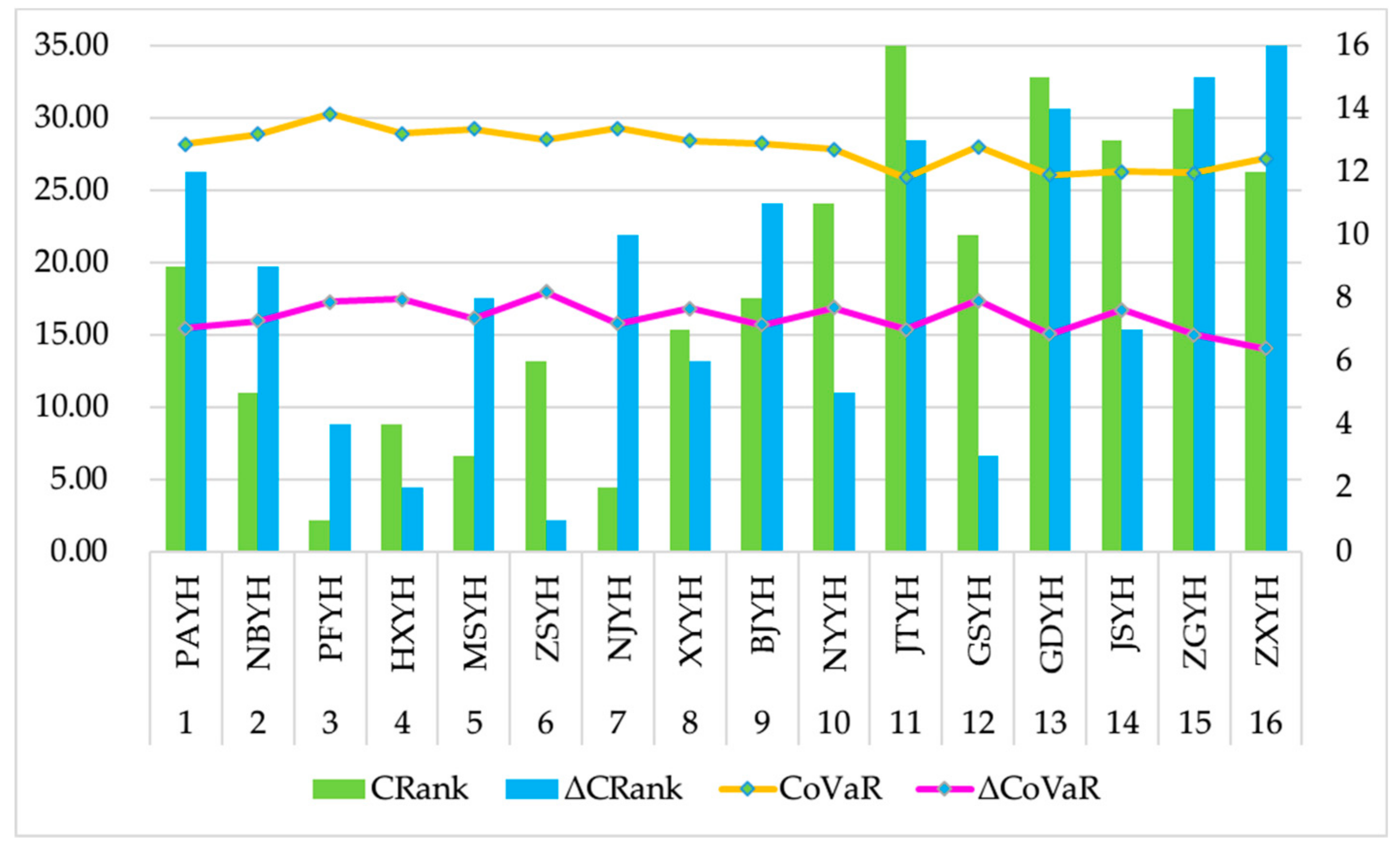
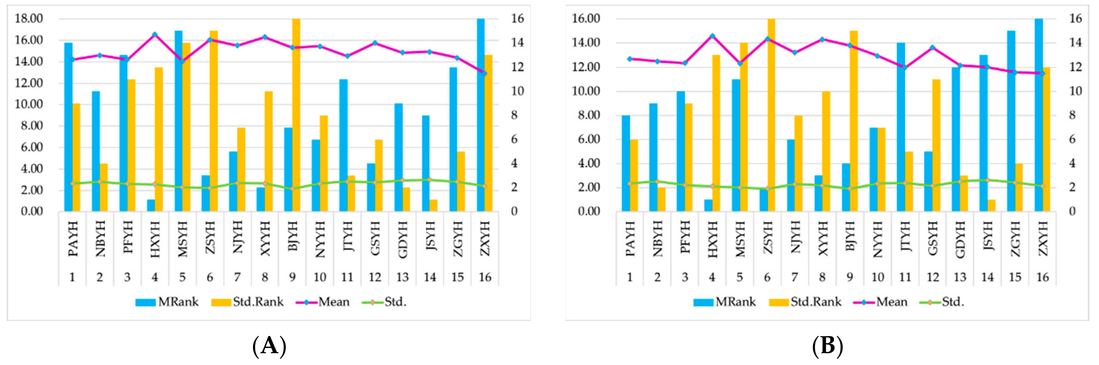
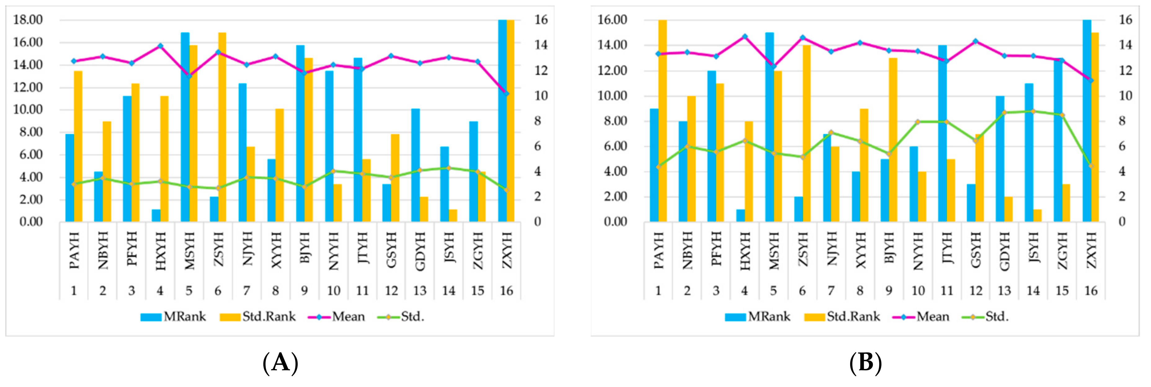
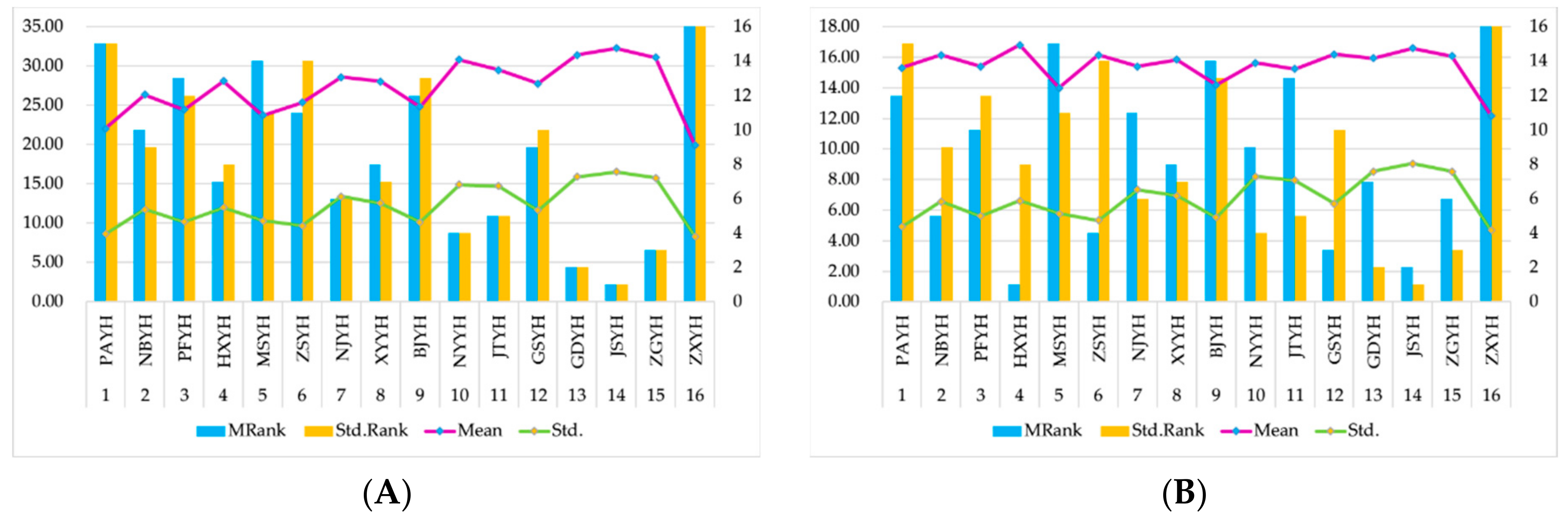
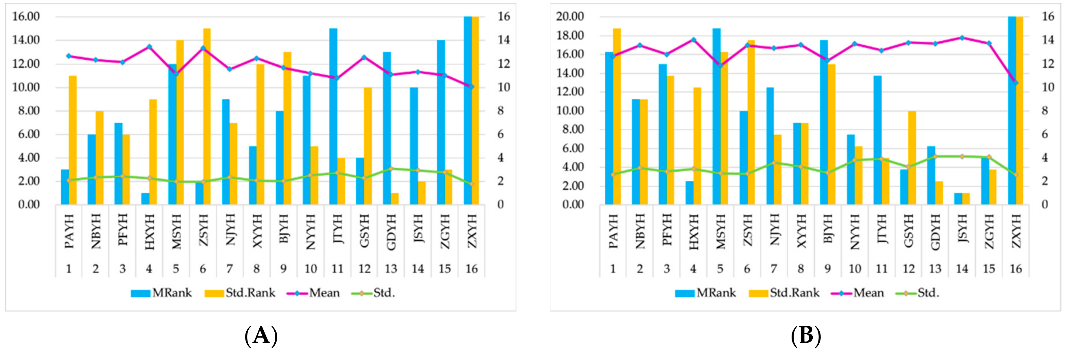
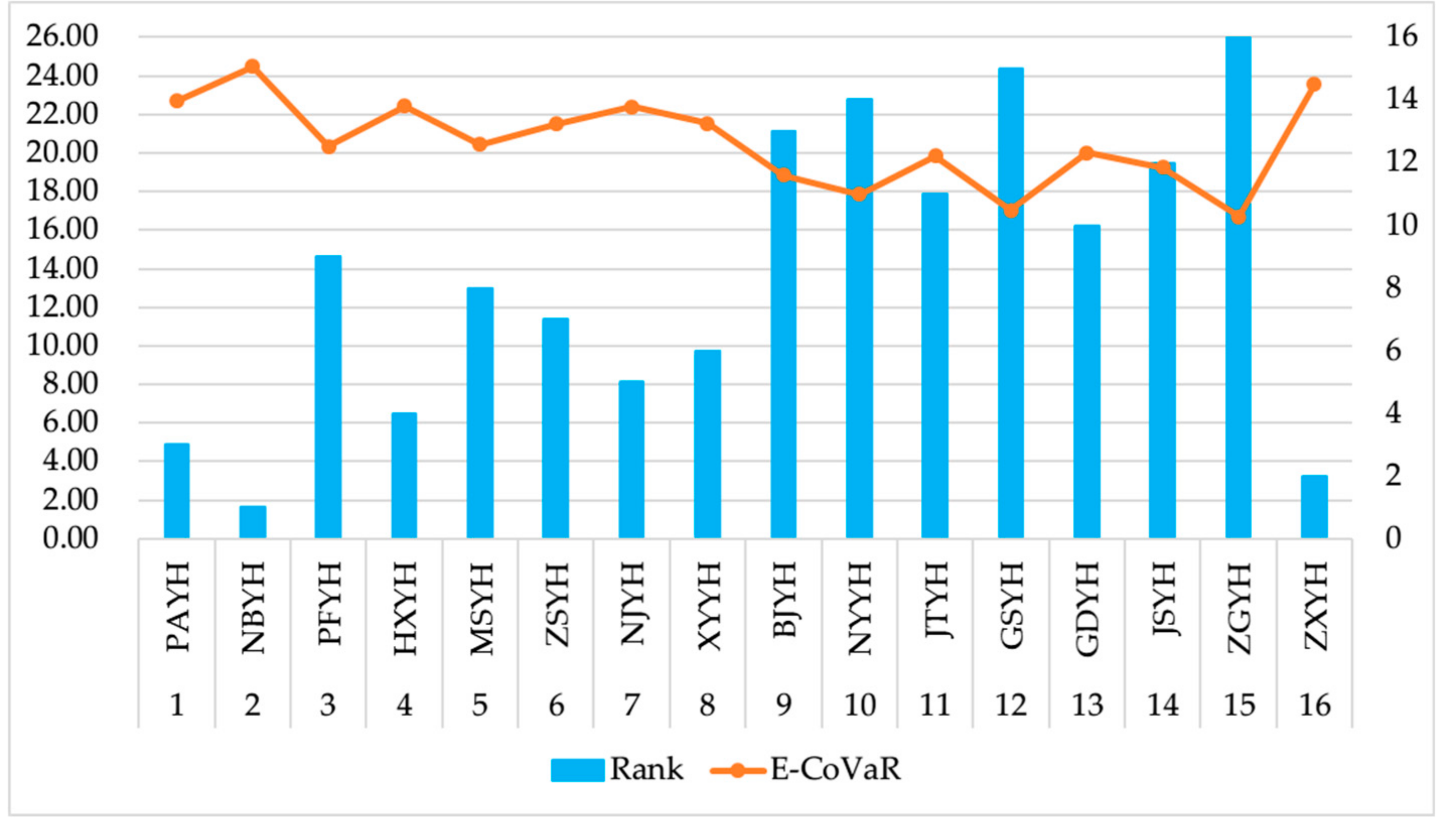
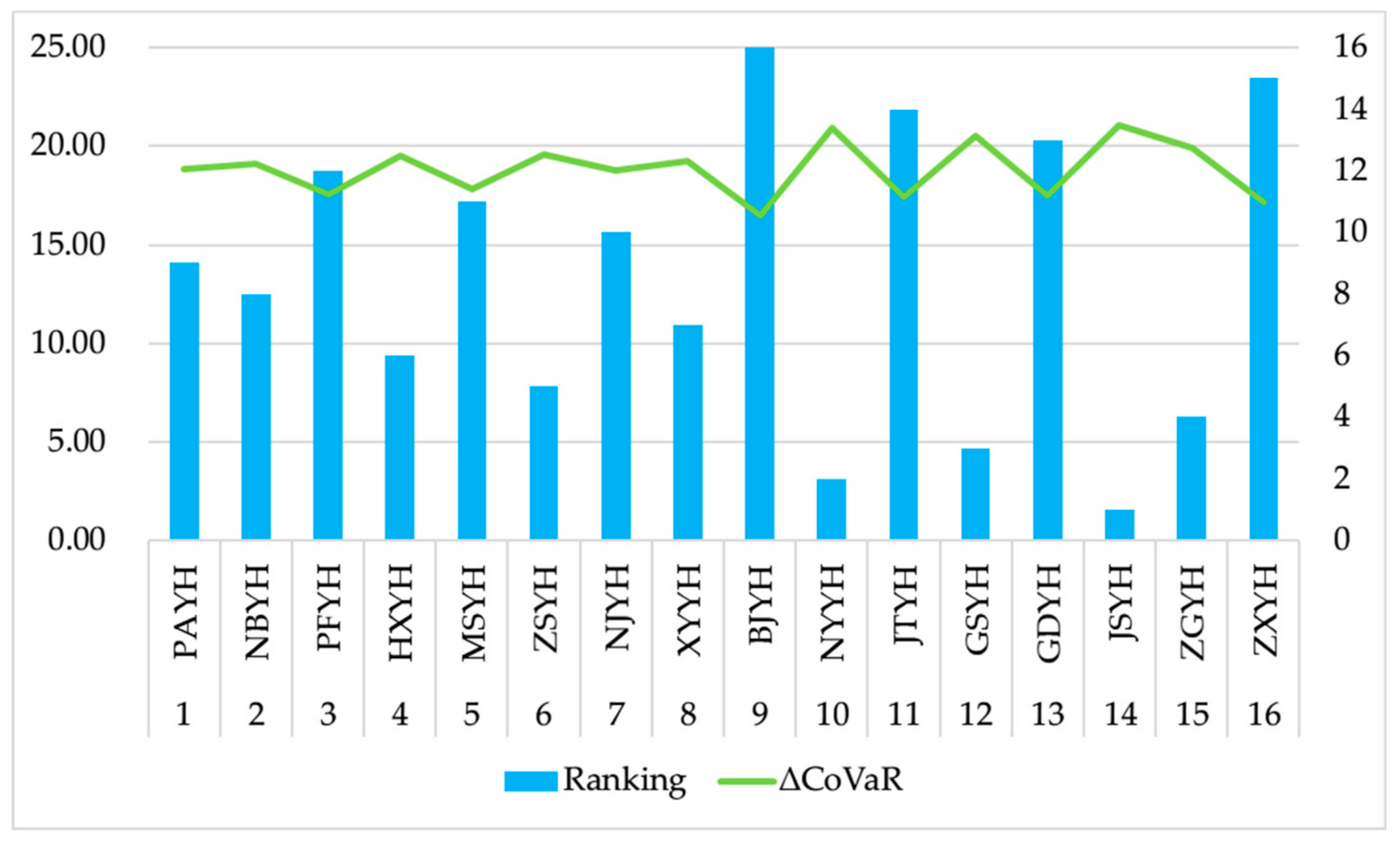
First, the market-based CoVaR approach, which is a useful complement for the indicator approach, could provide more information for strengthening financial supervision than the traditional indicator approach. The indicator system as well as the statistical tests clearly shows that the systemically important banks identified by the indicator approach are always big banks. However, we can conclude that for China, the systemic importance of a bank could not be simplified as the bank size rankings. Besides, the bank size rankings are not always positive and sometimes even negatively correlated with the rankings of systemic risk indicators (i.e., rankings of systemic importance) in the digital economy era. The conclusion still holds true when we assume that a bank is in extreme circumstance or considers the effects of Fintech and non-bank financial institutions.

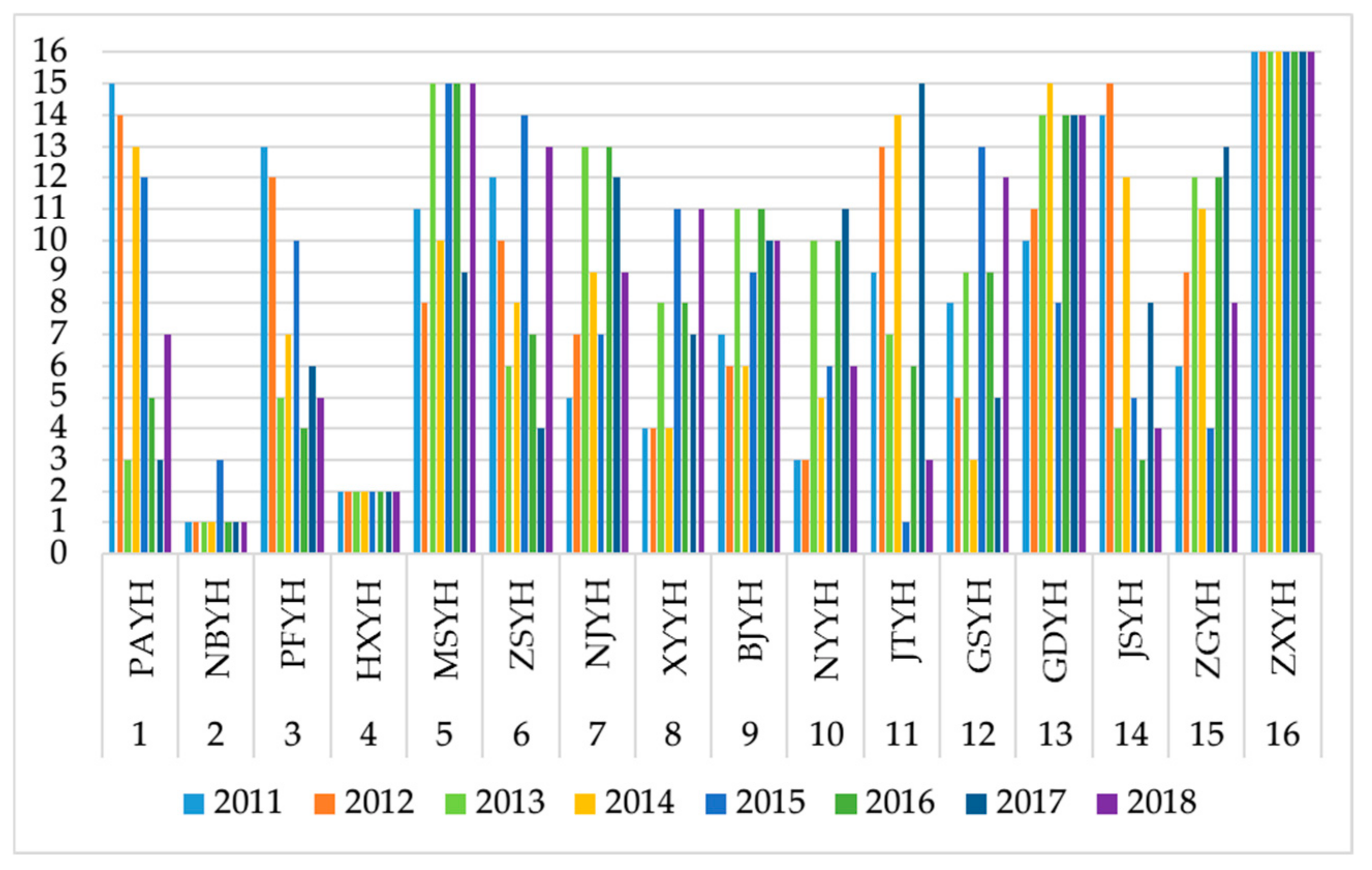
Second, the systemic risk changes over time. Based on the CoVaR models, we measure the systemic risk of 16 listed banks from 2011 to 2018, year by year, and integrate an overall analysis of the sample banks during the entire sample period. It is found that the levels of systemic risk vary across different time periods with the changes in domestic and international economic and financial situations. In the era of the digital economy, information transfers faster than before and customers can enjoy the benefits in the era, while we also need to know that the risk could also transfer faster. The periodical assessment of the systemic risk in the digital economy era could provide on timely early warning for regulators to avoid the accumulation of the risk and the occurrence of a crisis.

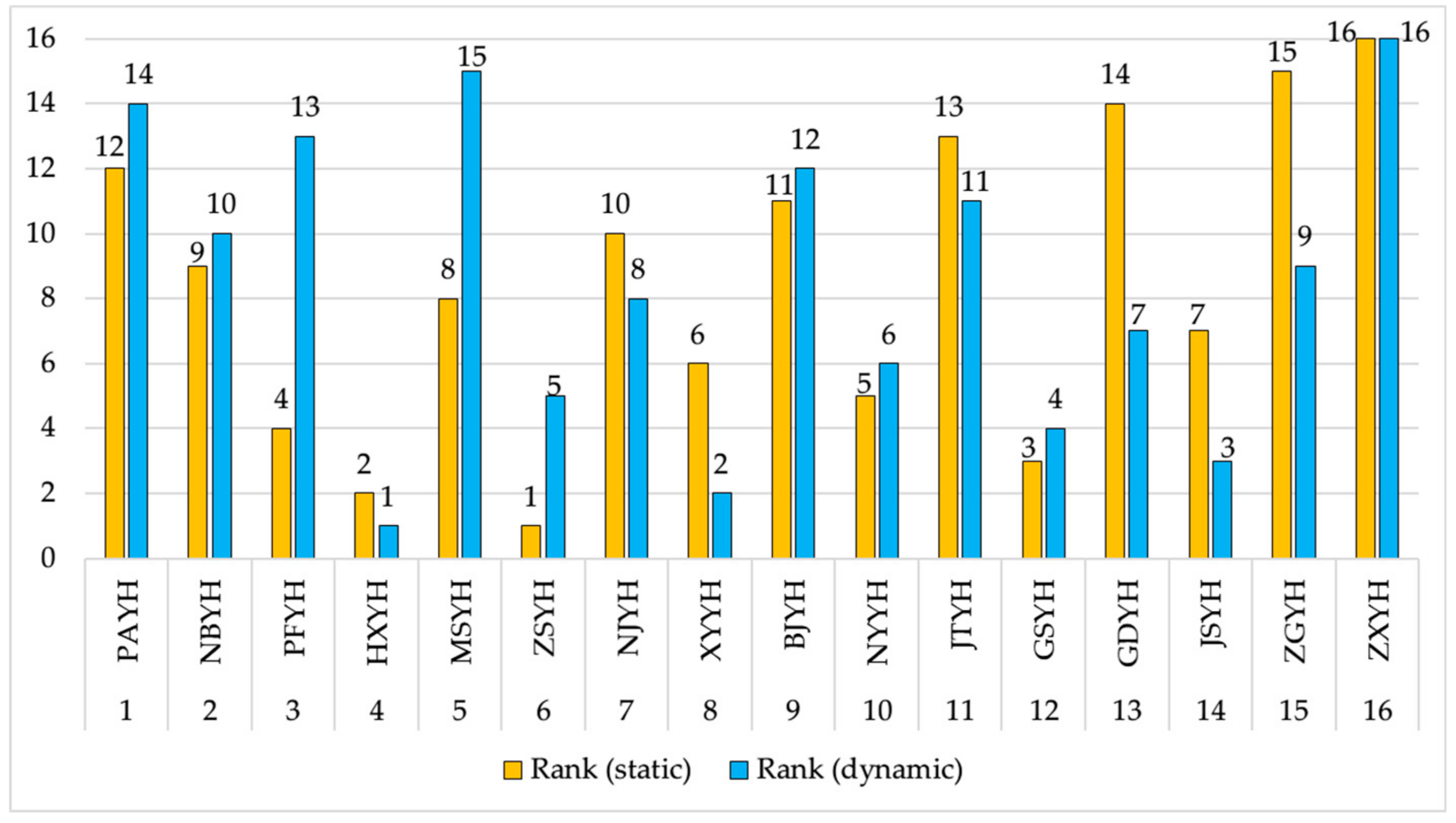
Third, based on both the static CoVaR model and the dynamic CoVaR models which introduce the state variables, the systemic importance rankings of banks change over time. Therefore, we suggest that the financial supervision of SIFIs requires dynamic evaluation, and the dynamic model is an enhanced model of the traditional static model, which contains more information and is time-varying, and it should be further developed for financial supervision. Furthermore, for China, the year-by-year analyses show that systemically important banks change over time, especially the bank which contributes the most to systemic risk. Interestingly, some SOE banks (big banks) are systemically important, and these banks are also identified by the indicator approach due to their huge sizes. However, the results based on the market data indicate that some SOE banks are not always systemically important, and some JOI and CCB banks (small banks) are identified as the systemically important banks. The base and extended models support the following view, which coincides with the point that we propose in the introduction section: small banks could also contribute to systemic risk and cause a systemic effect in the digital economy era. We contribute to the existing studies with empirical evidence and theoretical analysis.

Overall, we suggest that in the digital economy era, the measurement of systemic risk and the identification of systemically important banks should be based on more and more market-based approaches, including the CoVaR model. Besides, with the development of Fintech and non-bank financial institutions, we should develop more models that incorporate the effects of these financial activities. In addition, the financial supervision, especially the reform of the macroprudential framework, should deeply consider the systemic risk contributions of not only big banks but also small banks, which may be not as large as the SOE banks in China but remain systemically important to the banking system. Differential supervision should be further developed to maintain financial stability not only in China but also around the world.

References

1. Tapscott, D. The Digital Economy: Promise and Peril in the Age of Networked Intelligence, 1st ed.; McGraw-Hill: New York, NY, USA, 1995; pp. 1–368. [Google Scholar]
2. Tapscott, D. The Digital Economy Anniversary Edition: Rethinking Promise and Peril in the Age of Networked Intelligence, 2nd ed.; McGraw-Hill: New York, NY, USA, 2014; pp. 1–449. [Google Scholar]
3. G20 Digital Economy Development and Cooperation Initiative. Available online: http://www.g20chn.org/English/Documents/Current/201609/P020160908736971932404.pdf (accessed on 20 September 2018).
4. Measuring the Digital Economy. Available online: https://www.imf.org/~/media/Files/Publications/PP/2018/022818MeasuringDigitalEconomy.ashx (accessed on 28 February 2018).
5. Greene, E.F.; McIlwain, K.L.; Scott, J.T. A closer look at “too big to fail”: National and international approaches to addressing the risks of large, interconnected financial institutions. Cap. Mark. Law J. 2010, 5, 117–140. [Google Scholar] [CrossRef]
6. Xi Launches Financial Reforms. Available online: http://www.chinadaily.com.cn/china/2017-07/17/content_30135404.htm (accessed on 20 August 2017).
7. Secure a Decisive Victory in Building a Moderately Prosperous Society in All Respects and Strive for the Great Success of Socialism with Chinese Characteristics for a New Era. Available online: http://english.qstheory.cn/2018-02/11/c_1122395333.htm (accessed on 26 March 2018).
8. China Improves Supervision of Systemically Important Financial Institutions. Available online: http://en.people.cn/n3/2018/1128/c90000-9522675.html (accessed on 1 December 2018).
9. The Organization Structure of People’s Bank of China. Available online: http://www.gov.cn/xinwen/2019-02/02/content_5363338.htm (accessed on 12 February 2019).
10. PBC Launched the Pilot of Supervision on Fintech Innovations. Available online: http://www.gov.cn/xinwen/2019-12/06/content_5458990.htm (accessed on 31 December 2019).
11. Li, D.K. Banking Industry Contributed the Most to China’s Systemic Risk. Insight China 2012, 6, 18. Available online: https://kns.cnki.net/KCMS/detail/detail.aspx?dbcode=CJFQ&dbname=CJFDN1214&filename=KACZ201206009 (accessed on 6 January 2019).
12. 2019 List of Global Systemically Important Banks (G-SIBs). Available online: https://www.fsb.org/wp-content/uploads/P221119-1.pdf (accessed on 26 November 2019).
13. China’s Economic Development in the Past 70 Years. Available online: http://economy.gmw.cn/2019-09/26/content_33189822.htm (accessed on 30 September 2019).
14. The Total Assets of China’s Banking Financial Institutions Reached 268 Trillion RMB. Available online: http://finance.china.com.cn/news/20190225/4905682.shtml (accessed on 25 February 2019).
15. The Top 1000 World Banks (2019). Available online: https://www.thebanker.com/Top-1000 (accessed on 30 June 2019).
16. Jiang, H.C.; He, Y.F. Applying Data Envelopment Analysis in Measuring the Efficiency of Chinese Listed Banks in The Context of Macroprudential Framework. Mathematics 2018, 6, 184. [Google Scholar] [CrossRef] [Green Version]
17. Khiari, W.; Ben Sassi, S. On Identifying the Systemically Important Tunisian Banks: An Empirical Approach Based on the ΔCoVaR Measures. Risks 2019, 7, 122. [Google Scholar] [CrossRef] [Green Version]
18. Xu, C. The Literature Review of the Methods Related to the Identification of Systemically Important Financial Institutions. Stud. Int. Financ. 2011, 11, 57–64. Available online: https://kns.cnki.net/KCMS/detail/detail.aspx?dbcode=CJFQ&dbname=CJFD2011&filename=GJJR201111008 (accessed on 2 November 2017).
19. A Framework for Dealing with Domestic Systemically Important Banks. Available online: https://www.bis.org/publ/bcbs233.pdf (accessed on 6 June 2017).
20. Global Systemically Important Banks: Updated Assessment Methodology and the Higher Loss Absorbency Requirement. Available online: https://www.bis.org/publ/bcbs233.pdf (accessed on 2 February 2018).
21. Adrian, T.; Brunnermeier, M.K. CoVaR. NBER Working Paper 2011, 10, 1–45. [Google Scholar] [CrossRef]
22. Adrian, T.; Brunnermeier, M.K. CoVaR. Am. Econ. Rev. 2016, 106, 1705–1741. [Google Scholar] [CrossRef]
23. Drakos, A.A.; Kouretas, G.P. Bank Ownership, Financial Segments and the Measurement of Systemic Risk: An Application of CoVaR. Int. Rev. Econ. Financ. 2015, 40, 127–140. [Google Scholar] [CrossRef]
24. Deng, X.F. Research on the Return and Spillover Effect of the Financial industry. Contemp. Econ. 2019, 2, 27–30. Available online: https://kns.cnki.net/KCMS/detail/detail.aspx?dbcode=CJFQ&dbname=CJFDLAST2019&filename=DAJJ201902010 (accessed on 16 February 2018).
25. Wang, W.; Zhang, Y.; Wang, Y.X. The Measurement of Systemic Risk Based on Dynamic CoVaR and the Research on Financial Regulation. Financ. Theory Pract. 2018, 12, 47–54. Available online: https://kns.cnki.net/KCMS/detail/detail.aspx?dbcode=CJFQ&dbname=CJFDLAST2019&filename=JRLS201812008 (accessed on 16 December 2018).
26. Verma, R.; Ahmad, W.; Uddin, G.S.; Bekiros, S. Analysing the Systemic Risk of Indian banks. Econ. Lett. 2019, 176, 103–108. [Google Scholar] [CrossRef]
27. Girardi, G.; Ergün, A.T. Systemic Risk Measurement: Multivariate GARCH Estimation of CoVaR. J. Bank. Financ. 2013, 37, 3169–3180. [Google Scholar] [CrossRef]
28. López-Espinosa, G.; Moreno, A.; Rubia, A.; Valderrama, L. Short-Term Wholesale Funding and Systemic Risk: A Global CoVaR Approach. J. Bank. Financ. 2012, 36, 3150–3162. [Google Scholar] [CrossRef] [Green Version]
29. Zheng, D.; Yan, Y.R.; Lei, L. The Spillover Effect of Liquidity Risk in China’s Commercial Banks: A Dynamic CoVaR Approach. Financ. Econ. 2019, 1, 39–51. Available online: https://kns.cnki.net/KCMS/detail/detail.aspx?dbcode=CJFQ&dbname=CJFDLAST2019&filename=CJKX201901005 (accessed on 2 February 2019).
30. Reboredo, J.C.; Ugolini, A. Systemic Risk in European Sovereign Debt Markets: A CoVaR-copula Approach. J. Int. Money Financ. 2015, 51, 214–244. [Google Scholar] [CrossRef]
31. Bernal, O.; Gnabo, J.Y.; Guilmin, G. Economic Policy Uncertainty and Risk Spillovers in the Eurozone. J. Int. Money Financ. 2016, 65, 24–45. [Google Scholar] [CrossRef]
32. Scaillet, O. Nonparametric Estimation of Conditional Expected Shortfall. Insur. Risk Manag. J. 2005, 74, 639–660. Available online: https://archive-ouverte.unige.ch/unige:41796/ATTACHMENT01 (accessed on 26 July 2018).
33. Chen, S.D.; Wang, Y. Measuring Systemic Financial Risk of China’s Financial Institution. Chin. J. Manag. Sci. 2014, 22, 10–17. [Google Scholar] [CrossRef]
34. Tian, J.; Wang, Q. Bank Capital Constraints, Risk Spillover, and Systematic Financial Risk. Financ. Trade Econ. 2015, 8, 74–90. [Google Scholar] [CrossRef]
35. Mai, M.R.; Peng, T. Research on Systemic Risk Spillover of Listed Commercial Banks Based on CoVaR. Contemp. Econ. 2017, 30, 123–125. Available online: https://kns.cnki.net/KCMS/detail/detail.aspx?dbcode=CJFQ&dbname=CJFDLAST2017&filename=DAJJ201730048 (accessed on 26 January 2018).
36. Chen, G.J.; Zhong, L.; Zhang, Y. Systemic Linkages in the Chinese Banking System. Syst. Eng. Theory Pract. 2017, 37, 61–79. Available online: https://kns.cnki.net/KCMS/detail/detail.aspx?dbcode=CJFQ&dbname=CJFDLAST2018&filename=XTLL201701005 (accessed on 22 January 2018).
37. National Statistical Data Released by the National Bureau of Statistics of China (NBSC). Available online: http://data.stats.gov.cn (accessed on 31 December 2019).
38. Yang, J.; Yu, Z.L.; Jia, Y.D.; Ma, J. The Transmission of Financial Shocks among China’s Financial Institutions: A Global Perspective. PBC Working Paper 2017, 4, 1–29. Available online: http://www.cnfinance.cn/uploads/upload_files/file/201705/201705101629298215.pdf (accessed on 20 August 2018).
39. De Souza, S.R.S.; Silva, T.C.; Tabak, B.M.; Guerra, S.M. Evaluating Systemic Risk Using Bank Default Probabilities in Financial Networks. J. Econ. Dyn. Control 2016, 66, 54–75. [Google Scholar] [CrossRef]
40. Ouyang, H.B.; Kang, X.K. The Analysis of the Interconnectedness of Chinese Listed Banks and the Evolution of the Network Structure. South China Financ. 2017, 7, 14–26. Available online: https://kns.cnki.net/KCMS/detail/detail.aspx?dbcode=CJFQ&dbname=CJFDLAST2017&filename=GDJR201707003 (accessed on 26 February 2018).
41. Acharya, V.V.; Yorulmazer, T. Too Many to Fail—An Analysis of Time-Inconsistency in Bank Closure Policies. J. Financ. Intermed. 2007, 16, 1–31. [Google Scholar] [CrossRef]
42. Varotto, S.; Zhao, L. Systemic Risk and Bank Size. J. Int. Money Financ. 2018, 82, 45–70. [Google Scholar] [CrossRef]
43. Manguzvane, M.; Muteba Mwamba, J.W. Modelling Systemic Risk in the South African Banking Sector Using CoVaR. Int. Rev. Appl. Econ. 2019, 33, 1–18. [Google Scholar] [CrossRef]
44. Chen, Z.Y.; Liu, Z.Y. Do State-owned Large Commercial Banks Contribute More to Systemic Risk? Financ. Trade Econ. 2013, 9, 57–66. [Google Scholar] [CrossRef]
Figure 1. The indicator approach.
Mathematics 08 00180 g001
Figure 2. The results (The left axis refers to the values of the CoVaR and ΔCoVaR of each bank, and the right axis refers to the rankings of the bank in terms of CoVaR and ΔCoVaR. We use the same formation from Figure 2 to Figure 6) of CoVaR and ΔCoVaR (In the figure, the CoVaR refers to the Conditional Value at Risk when a bank is in distress; ΔCoVaR refers to the difference between the CoVaRs when the bank is in distress and in a normal state): (A) 2011; (B) 2012.
Mathematics 08 00180 g002
Figure 3. The results of CoVaR and ΔCoVaR (In the figure, the CoVaR refers to the Conditional Value at Risk when a bank is in distress; ΔCoVaR refers to the difference between the CoVaRs when the bank is in distress and in a normal state): (A) 2013; (B) 2014.
Mathematics 08 00180 g003
Figure 4. The results of CoVaR and ΔCoVaR (In the figure, the CoVaR refers to the Conditional Value at Risk when a bank is in distress; ΔCoVaR refers to the difference between the CoVaRs when the bank is in distress and in a normal state): (A) 2015; (B) 2016.
Mathematics 08 00180 g004
Figure 5. The results of CoVaR and ΔCoVaR (In the figure, the CoVaR refers to the Conditional Value at Risk when a bank is in distress; ΔCoVaR refers to the difference between the CoVaRs when the bank is in distress and in a normal state): (A) 2017; (B) 2018.
Mathematics 08 00180 g005
Figure 6. The overall results of CoVaR and ΔCoVaR (In the figure, the CoVaR refers to the Conditional Value at Risk when a bank is in distress; ΔCoVaR refers to the difference between the CoVaRs when the bank is in distress and in a normal state) (2011–2018).
Mathematics 08 00180 g006
Figure 7. The results (The left axis refers to the values of the mean and standard deviation of each bank’s ΔCoVaR, and the right axis refers to the rankings of the bank in terms of the mean and standard deviation of ΔCoVaR. We use the same formation from Figure 7 to Figure 11) of the mean and standard deviations of ΔCoVaR (In the figure, we calculate the daily ΔCoVaR (the difference between the Conditional Value at Risk (CoVaRs) when the bank is in distress and in a normal state) of each bank, and then derive the corresponding mean and standard deviation for each bank): (A) 2011; (B) 2012.
Mathematics 08 00180 g007
Figure 8. The results of the mean and standard deviations of ΔCoVaR (In the figure, we calculate the daily ΔCoVaR (the difference between the Conditional Value at Risk (CoVaRs) when the bank is in distress and in a normal state) of each bank, and then derive the corresponding mean and standard deviation for each bank): (A) 2013; (B) 2014.
Mathematics 08 00180 g008
Figure 9. The results of the mean and standard deviations of ΔCoVaR (In the figure, we calculate the daily ΔCoVaR (the difference between the Conditional Value at Risk (CoVaRs) when the bank is in distress and in a normal state) of each bank, and then derive the corresponding mean and standard deviation for each bank): (A) 2015; (B) 2016.
Mathematics 08 00180 g009
Figure 10. The results of the mean and standard deviations of ΔCoVaR (In the figure, we calculate the daily ΔCoVaR (the difference between the Conditional Value at Risk (CoVaRs) when the bank is in distress and in a normal state) of each bank, and then derive the corresponding mean and standard deviation for each bank): (A) 2017; (B) 2018.
Mathematics 08 00180 g010
Figure 11. The overall results of the mean and standard deviations of ΔCoVaR (In the figure, we calculate the daily ΔCoVaR (the difference between the Conditional Value at Risk (CoVaRs) when the bank is in distress and in a normal state) of each bank, and then derive the corresponding mean and standard deviation for each bank): (2011–2018).
Mathematics 08 00180 g011
Figure 12. Comparison: measurements (The left axis refers to the rankings based on the overall results derived from two models) of static and dynamic ΔCoVaR (In the figure, ΔCoVaR refers to the difference between the Conditional Value at Risk (CoVaRs) when the bank is in distress and in a normal state).
Mathematics 08 00180 g012
Figure 13. Measurements of dynamic ΔCoVaRs (The left axis refers to the value of ΔCoVaR (the difference between the Conditional Value at Risk (CoVaRs) when the bank is in distress and in a normal state) of each bank, based on the dynamic model which considers extreme circumstance and use a 1% quantile) (2011–2018, extreme circumstance).
Mathematics 08 00180 g013
Figure 14. Rankings of dynamic ΔCoVaR (The left axis refers to the ranking of each bank in terms of ΔCoVaR (the difference between the Conditional Value at Risk (CoVaRs) when the bank is in distress and in a normal state), based on the dynamic model which considers extreme circumstance and use a 1% quantile) (2011–2018, extreme circumstance).
Mathematics 08 00180 g014
Figure 15. Measurements and rankings of dynamic ΔCoVaRs (overall analysis, extreme circumstance) (The left axis and right axis refers to the value and ranking of the dynamic ΔCoVaR (the difference between the Conditional Value at Risk (CoVaRs) when the bank is in distress and in a normal state) of each bank).
Mathematics 08 00180 g015
Figure 16. Measurements and rankings of Exposure ΔCoVaRs (The left axis and right axis refers to the value and ranking of the Exposure ΔCoVaR (the difference between the Exposure Conditional Value at Risk (CoVaRs) when the banking system is in distress and in a normal state) of each bank during the entire sample period) (overall analysis, exposure model).
Mathematics 08 00180 g016
Figure 17. Measurements and rankings of dynamic ΔCoVaRs (The left axis and right axis refers to the value and ranking of the dynamic ΔCoVaR (the difference between the Conditional Value at Risk (CoVaRs) when the banking system is in distress and in a normal state) of each bank, based on the modified dynamic model which incorporates the effects of Fintech and non-bank financial institutions during the sample period of 2015–2018) (overall analysis, modified model).
Mathematics 08 00180 g017
Figure 18. Measurements (The “size”, “interc”, “subs” and “complx” respectively refer to the values of the four indicators including size, interconnectedness, substitutability and complexity of a bank; the “systemic importance” refers to the measurement of the systemic importance of the banks based on the weighted average values of the four types of indicators; the “rankings” represents the ranking of a bank in terms of the systemic importance) and rankings (The left axis and right axis refers to the systemic risk evaluation and ranking of each bank, based on the indicator approach during the entire sample period) of systemic risk (the indicator approach).
Mathematics 08 00180 g018