Resilience-Based Restoration Model for Supply Chain Networks

Abstract
1. Introduction
2. Literature Review
3. Methodology
3.1. Assumption
- (1)
- Each disrupted link in the supply chain network is not operational until it is completely recovered.
- (2)
- All supplies are delivered from the supply nodes to the demand nodes through the fastest path in the network.
- (3)
- Each work crew can only work on the restoration of a disrupted link at a time.
- (4)
- Each link is restored only by one work crew.
- (5)
- Each restoration activity is non-preemptive, i.e., each restoration activity is implemented only once over the restoration time horizon.
- (6)
- The amount of demands from supply nodes to demand nodes is fixed and does not vary over the restoration time horizon.
3.2. Notation
3.3. Problem Statement
3.4. Resilience Metrics
3.4.1. Resilience of Cumulative Loss
3.4.2. Resilience of Restoration Rapidity
3.5. Modeling
3.6. Model Solution
| Algorithm 1 Pseudo code of SA procedure |
| //Initialization Randomly generate an initial solution , and the initial objection function value is ; ; w=0; //The outer iteration times ; //Initial Temperature ; //Freezing Temperature while not stop //The search loop under the temperature for l = 1 to L //The inner iteration times Generate a new feasible solution based on the current solution , and calculate the objection function value . if ; if ; ; continues; end if Calculate the acceptance probability ; if random(0,1) < P ; end if end for //Drop down the temperature ; =+1 end while end procedure |
4. Case Study
4.1. Supply Chain Network and Basic Data
4.2. Results
4.2.1. Pre-Disruption Path
4.2.2. Optimal Restoration Schedule
4.3. Sensitivity Analysis
4.3.1. Decision-Maker’s Preference
4.3.2. Tolerance Factor of Delivery Time
4.3.3. Number of Work Crews
4.3.4. Availability of Budget
5. Conclusions
- (1)
- The proposed method framework can generate an efficient restoration strategy from a perspective of resilience considering the tradeoff between the cumulative performance loss and the restoration rapidity, which can provide an effective reference for decision-makers to schedule the restoration activities for a disrupted supply chain network.
- (2)
- Decision-maker’s preference has a great impact on the road segments to be repaired and the time sequence of restoration activities. With an increase of the tolerance factor of delivery time, the resilience of the supply chain network increase with different rates but the total restoration costs, makespan, and the number of road segments to be restored all decrease.
- (3)
- More work crews can shorten the makespan and increase the resilience but may decrease the marginal benefit of manpower resources when the number of work crews exceeds a certain level. Likewise, more availability of budget can improve the supply chain network performance but increasing budget alone and keeping the number of work crews constant cannot improve the restoration schedule when the monetary resources exceed a certain level.
Author Contributions
Funding
Conflicts of Interest
References
- Crainic, T.G. Service network design in freight transportation. Eur. J. Oper. Res. 2000, 122, 272–288. [Google Scholar] [CrossRef]
- Miller-Hooks, E.; Zhang, X.; Faturechi, R. Measuring and maximizing resilience of freight transportation networks. Comput. Oper. Res. 2012, 39, 1633–1643. [Google Scholar] [CrossRef]
- SteadieSeifi, M.; Dellaert, N.P.; Nuijten, W.; Van Woensel, T.; Raoufi, R. Multimodal freight transportation planning: A literature review. Eur. J. Oper. Res. 2014, 233, 1–15. [Google Scholar] [CrossRef]
- Darayi, M.; Barker, K.; Santos, J.R. Component importance measures for multi-industry vulnerability of a freight transportation network. Netw. Spat. Econ. 2017, 17, 1111–1136. [Google Scholar] [CrossRef]
- Zhu, E.; Crainic, T.G.; Gendreau, M. Scheduled service network design for freight rail transportation. Oper. Res. 2014, 62, 383–400. [Google Scholar] [CrossRef]
- Wang, S.; Sarker, B.R.; Mann, L., Jr.; Triantaphyllou, E. Resource planning and a depot location model for electric power restoration. Eur. J. Oper. Res. 2004, 155, 22–43. [Google Scholar] [CrossRef]
- Matisziw, T.C.; Murray, A.T.; Grubesic, T.H. Strategic network restoration. Netw. Spat. Econ. 2010, 10, 345–361. [Google Scholar] [CrossRef]
- Zhang, C.; Kong, J.-J.; Simonovic, S.P. Restoration resource allocation model for enhancing resilience of interdependent infrastructure systems. Saf. Sci. 2018, 102, 169–177. [Google Scholar] [CrossRef]
- Karakoc, D.B.; Almoghathawi, Y.; Barker, K.; González, A.D.; Mohebbi, S. Community resilience-driven restoration model for interdependent infrastructure networks. Int. J. Disaster Risk Reduct. 2019, 38, 101228. [Google Scholar] [CrossRef]
- Lambrechts, O.; Demeulemeester, E.; Herroelen, W. Proactive and reactive strategies for resource-constrained project scheduling with uncertain resource availabilities. J. Sched. 2008, 11, 121–136. [Google Scholar] [CrossRef]
- Nurre, S.G.; Cavdaroglu, B.; Mitchell, J.E.; Sharkey, T.C.; Wallace, W.A. Restoring infrastructure systems: An integrated network design and scheduling (INDS) problem. Eur. J. Oper. Res. 2012, 223, 794–806. [Google Scholar] [CrossRef]
- Li, Z.; Jin, C.; Hu, P.; Wang, C. Resilience-based transportation network recovery strategy during emergency recovery phase under uncertainty. Reliab. Eng. Syst. Saf. 2019, 188, 503–514. [Google Scholar] [CrossRef]
- Cho, S.; Gordon, P.; Richardson, H.W.; Moore, J.E.; Shinozuka, M. Analyzing transportation reconstruction network strategies: A full cost approach. Rev. Urban Reg. Dev. Stud. 2000, 12, 212–227. [Google Scholar] [CrossRef]
- Çelik, M. Network restoration and recovery in humanitarian operations: Framework, literature review, and research directions. Surv. Oper. Res. Manag. Sci. 2016, 21, 47–61. [Google Scholar] [CrossRef]
- Ciric, R.M.; Popovic, D.S. Multi-objective distribution network restoration using heuristic approach and mix integer programming method. Int. J. Electr. Power Energy Syst. 2000, 22, 497–505. [Google Scholar] [CrossRef]
- Xu, M.; Ouyang, M.; Mao, Z.; Xu, X. Improving repair sequence scheduling methods for postdisaster critical infrastructure systems. Comput. Aided Civ. Infrastruct. Eng. 2019, 34, 506–522. [Google Scholar] [CrossRef]
- Liu, C.; Fan, Y.; Ordóñez, F. A two-stage stochastic programming model for transportation network protection. Comput. Oper. Res. 2009, 36, 1582–1590. [Google Scholar] [CrossRef]
- Chen, L.; Miller-Hooks, E. Resilience: An indicator of recovery capability in intermodal freight transport. Transp. Sci. 2012, 46, 109–123. [Google Scholar] [CrossRef]
- Karlaftis, M.G.; Kepaptsoglou, K.L.; Lambropoulos, S. Fund allocation for transportation network recovery following natural disasters. J. Urban Plan. Dev. 2007, 133, 82–89. [Google Scholar] [CrossRef]
- Hackl, J.; Adey, B.T.; Lethanh, N. Determination of near-optimal restoration programs for transportation networks following natural hazard events using simulated annealing. Comput. Aided Civ. Infrastruct. Eng. 2018, 33, 618–637. [Google Scholar] [CrossRef]
- Nagata, T.; Sasaki, H. A multi-agent approach to power system restoration. IEEE Trans. Power Syst. 2002, 17, 457–462. [Google Scholar] [CrossRef]
- Tabucchi, T.; Davidson, R.; Brink, S. Simulation of post-earthquake water supply system restoration. Civ. Eng. Environ. Syst. 2010, 27, 263–279. [Google Scholar] [CrossRef]
- Fang, Y.; Sansavini, G. Emergence of antifragility by optimum postdisruption restoration planning of infrastructure networks. J. Infrastruct. Syst. 2017, 23, 04017024. [Google Scholar] [CrossRef]
- González, A.D.; Dueñas-Osorio, L.; Sánchez-Silva, M.; Medaglia, A.L. The interdependent network design problem for optimal infrastructure system restoration. Comput. Aided Civ. Infrastruct. Eng. 2016, 31, 334–350. [Google Scholar] [CrossRef]
- Fang, Y.-P.; Sansavini, G. Optimum post-disruption restoration under uncertainty for enhancing critical infrastructure resilience. Reliab. Eng. Syst. Saf. 2019, 185, 1–11. [Google Scholar] [CrossRef]
- Sanci, E.; Daskin, M.S. Integrating location and network restoration decisions in relief networks under uncertainty. Eur. J. Oper. Res. 2019, 279, 335–350. [Google Scholar] [CrossRef]
- Xu, N.; Guikema, S.D.; Davidson, R.A.; Nozick, L.K.; Çağnan, Z.; Vaziri, K. Optimizing scheduling of post-earthquake electric power restoration tasks. Earthq. Eng. Struct. Dyn. 2007, 36, 265–284. [Google Scholar] [CrossRef]
- Ransikarbum, K.; Mason, S.J. Multiple-objective analysis of integrated relief supply and network restoration in humanitarian logistics operations. Int. J. Prod. Res. 2016, 54, 49–68. [Google Scholar] [CrossRef]
- Schmitt, A.J.; Singh, M. A quantitative analysis of disruption risk in a multi-echelon supply chain. Int. J. Prod. Econ. 2012, 139, 22–32. [Google Scholar] [CrossRef]
- Carvalho, H.; Barroso, A.P.; Machado, V.H.; Azevedo, S.; Cruz-Machado, V. Supply chain redesign for resilience using simulation. Comput. Ind. Eng. 2012, 62, 329–341. [Google Scholar] [CrossRef]
- Xu, M.; Wang, X.; Zhao, L. Predicted supply chain resilience based on structural evolution against random supply disruptions. Int. J. Syst. Sci. Oper. Logist. 2014, 1, 105–117. [Google Scholar] [CrossRef]
- Hishamuddin, H.; Sarker, R.A.; Essam, D. A recovery model for a two-echelon serial supply chain with consideration of transportation disruption. Comput. Ind. Eng. 2013, 64, 552–561. [Google Scholar] [CrossRef]
- Deng, Y.; Chen, Y.; Zhang, Y.; Mahadevan, S. Fuzzy Dijkstra algorithm for shortest path problem under uncertain environment. Appl. Soft Comput. 2012, 12, 1231–1237. [Google Scholar] [CrossRef]
- Shin, K.; Shin, Y.; Kwon, J.-H.; Kang, S.-H. Development of risk based dynamic backorder replenishment planning framework using Bayesian Belief Network. Comput. Ind. Eng. 2012, 62, 716–725. [Google Scholar] [CrossRef]
- Almoghathawi, Y.; Barker, K.; Albert, L.A. Resilience-driven restoration model for interdependent infrastructure networks. Reliab. Eng. Syst. Saf. 2019, 185, 12–23. [Google Scholar] [CrossRef]
- Henry, D.; Ramirez-Marquez, J.E. Generic metrics and quantitative approaches for system resilience as a function of time. Reliab. Eng. Syst. Saf. 2012, 99, 114–122. [Google Scholar] [CrossRef]
- De, P.; Dunne, E.J.; Ghosh, J.B.; Wells, C.E. Complexity of the discrete time-cost tradeoff problem for project networks. Oper. Res. 1997, 45, 302–306. [Google Scholar] [CrossRef]
- Černý, V. Thermodynamical approach to the traveling salesman problem: An efficient simulation algorithm. J. Optim. Theory Appl. 1985, 45, 41–51. [Google Scholar] [CrossRef]
- Vincent, F.Y.; Redi, A.P.; Hidayat, Y.A.; Wibowo, O.J. A simulated annealing heuristic for the hybrid vehicle routing problem. Appl. Soft Comput. 2017, 53, 119–132. [Google Scholar]
- Ezugwu, A.E.-S.; Adewumi, A.O.; Frîncu, M.E. Simulated annealing based symbiotic organisms search optimization algorithm for traveling salesman problem. Expert Syst. Appl. 2017, 77, 189–210. [Google Scholar] [CrossRef]
- Ingber, L. Simulated annealing: Practice versus theory. Math. Comput. Model. 1993, 18, 29–57. [Google Scholar] [CrossRef]
- Vahdani, B.; Zandieh, M.; Roshanaei, V. A hybrid multi-stage predictive model for supply chain network collapse recovery analysis: A practical framework for effective supply chain network continuity management. Int. J. Prod. Res. 2011, 49, 2035–2060. [Google Scholar] [CrossRef]
- Das, K.; Chowdhury, A.H. Designing a reverse logistics network for optimal collection, recovery and quality-based product-mix planning. Int. J. Prod. Econ. 2012, 135, 209–221. [Google Scholar] [CrossRef]
- Ouyang, M.; Wang, Z. Resilience assessment of interdependent infrastructure systems: With a focus on joint restoration modeling and analysis. Reliab. Eng. Syst. Saf. 2015, 141, 74–82. [Google Scholar] [CrossRef]


| a | i | j | a | i | j | a | i | j | a | i | j | ||||
|---|---|---|---|---|---|---|---|---|---|---|---|---|---|---|---|
| 1 | 1 | 2 | 2.6 | 32 | 13 | 7 | 2.6 | 63 | 14 | 21 | 2.8 | 94 | 26 | 22 | 1.1 |
| 2 | 2 | 1 | 2.6 | 33 | 8 | 9 | 3.1 | 64 | 21 | 14 | 2.8 | 95 | 23 | 24 | 2.5 |
| 3 | 1 | 5 | 2.8 | 34 | 9 | 8 | 3.1 | 65 | 15 | 16 | 2.4 | 96 | 24 | 23 | 2.5 |
| 4 | 5 | 1 | 2.8 | 35 | 8 | 10 | 3.7 | 66 | 16 | 15 | 2.4 | 97 | 23 | 25 | 2.7 |
| 5 | 2 | 3 | 2.5 | 36 | 10 | 8 | 3.7 | 67 | 16 | 17 | 3.2 | 98 | 25 | 23 | 2.7 |
| 6 | 3 | 2 | 2.5 | 37 | 8 | 13 | 2.8 | 68 | 17 | 16 | 3.2 | 99 | 23 | 30 | 3.6 |
| 7 | 2 | 4 | 2.9 | 38 | 13 | 8 | 2.8 | 69 | 16 | 22 | 3.4 | 100 | 30 | 23 | 3.6 |
| 8 | 4 | 2 | 2.9 | 39 | 8 | 14 | 1.6 | 70 | 22 | 16 | 3.4 | 101 | 24 | 30 | 2.3 |
| 9 | 3 | 8 | 1.9 | 40 | 14 | 8 | 1.6 | 71 | 17 | 21 | 4.2 | 102 | 30 | 24 | 2.3 |
| 10 | 8 | 3 | 1.9 | 41 | 9 | 10 | 1.7 | 72 | 21 | 17 | 4.2 | 103 | 25 | 27 | 4.1 |
| 11 | 3 | 9 | 2.3 | 42 | 10 | 9 | 1.7 | 73 | 17 | 22 | 1.6 | 104 | 27 | 25 | 4.1 |
| 12 | 9 | 3 | 2.3 | 43 | 10 | 15 | 2.1 | 74 | 22 | 17 | 1.6 | 105 | 25 | 29 | 1.5 |
| 13 | 4 | 5 | 1.8 | 44 | 15 | 10 | 2.1 | 75 | 18 | 19 | 1.9 | 106 | 29 | 25 | 1.5 |
| 14 | 5 | 4 | 1.8 | 45 | 11 | 12 | 2.5 | 76 | 19 | 18 | 1.9 | 107 | 26 | 27 | 2.3 |
| 15 | 4 | 7 | 3.8 | 46 | 12 | 11 | 2.5 | 77 | 18 | 20 | 2.5 | 108 | 27 | 26 | 2.3 |
| 16 | 7 | 4 | 3.8 | 47 | 11 | 19 | 2.6 | 78 | 20 | 18 | 2.5 | 109 | 26 | 33 | 2.5 |
| 17 | 4 | 8 | 2.5 | 48 | 19 | 11 | 2.6 | 79 | 18 | 23 | 3.6 | 110 | 33 | 26 | 2.5 |
| 18 | 8 | 4 | 2.5 | 49 | 12 | 18 | 2.9 | 80 | 23 | 18 | 3.6 | 111 | 27 | 28 | 1.8 |
| 19 | 5 | 6 | 3.7 | 50 | 18 | 12 | 2.9 | 81 | 18 | 24 | 1.8 | 112 | 28 | 27 | 1.8 |
| 20 | 6 | 5 | 3.7 | 51 | 13 | 14 | 3.4 | 82 | 24 | 18 | 1.8 | 113 | 27 | 32 | 3.3 |
| 21 | 5 | 7 | 4.1 | 52 | 14 | 13 | 3.4 | 83 | 20 | 24 | 2.2 | 114 | 32 | 27 | 3.3 |
| 22 | 7 | 5 | 4.1 | 53 | 13 | 18 | 3.6 | 84 | 24 | 20 | 2.2 | 115 | 27 | 33 | 3.8 |
| 23 | 5 | 11 | 2.4 | 54 | 18 | 13 | 3.6 | 85 | 21 | 22 | 3.4 | 116 | 33 | 27 | 3.8 |
| 24 | 11 | 5 | 2.4 | 55 | 13 | 21 | 2.8 | 86 | 22 | 21 | 3.4 | 117 | 28 | 29 | 2.4 |
| 25 | 6 | 11 | 1.6 | 56 | 21 | 13 | 2.8 | 87 | 21 | 23 | 1.6 | 118 | 29 | 28 | 2.4 |
| 26 | 11 | 6 | 1.6 | 57 | 13 | 23 | 1.6 | 88 | 23 | 21 | 1.6 | 119 | 29 | 31 | 1.5 |
| 27 | 7 | 11 | 1.8 | 58 | 23 | 13 | 1.6 | 89 | 21 | 25 | 3.5 | 120 | 31 | 29 | 1.5 |
| 28 | 11 | 7 | 1.8 | 59 | 14 | 15 | 3.2 | 90 | 25 | 21 | 3.5 | 121 | 30 | 31 | 3.7 |
| 29 | 7 | 12 | 2.3 | 60 | 15 | 14 | 3.2 | 91 | 22 | 25 | 1.5 | 122 | 31 | 30 | 3.7 |
| 30 | 12 | 7 | 2.3 | 61 | 14 | 17 | 2.6 | 92 | 25 | 22 | 1.5 | 123 | 31 | 32 | 3.5 |
| 31 | 7 | 13 | 2.6 | 62 | 17 | 14 | 2.6 | 93 | 22 | 26 | 1.1 | 124 | 32 | 31 | 3.5 |
| k | O | D | k | O | D | k | O | D | |||
|---|---|---|---|---|---|---|---|---|---|---|---|
| 1 | 1 | 15 | 36 | 14 | 22 | 4 | 48 | 27 | 31 | 2 | 28 |
| 2 | 1 | 22 | 28 | 15 | 22 | 30 | 53 | 28 | 31 | 1 | 36 |
| 3 | 2 | 17 | 45 | 16 | 33 | 2 | 32 | 29 | 30 | 15 | 34 |
| 4 | 2 | 33 | 43 | 17 | 33 | 20 | 26 | 30 | 30 | 3 | 28 |
| 5 | 2 | 31 | 39 | 18 | 33 | 10 | 28 | 31 | 30 | 33 | 36 |
| 6 | 3 | 30 | 54 | 19 | 27 | 9 | 34 | 32 | 20 | 22 | 34 |
| 7 | 3 | 33 | 49 | 20 | 27 | 11 | 29 | 33 | 20 | 10 | 41 |
| 8 | 3 | 19 | 26 | 21 | 27 | 3 | 23 | 34 | 19 | 27 | 30 |
| 9 | 9 | 32 | 35 | 22 | 32 | 9 | 34 | 35 | 19 | 15 | 28 |
| 10 | 15 | 31 | 37 | 23 | 32 | 1 | 36 | 36 | 11 | 16 | 20 |
| 11 | 15 | 1 | 42 | 24 | 32 | 20 | 42 | 37 | 11 | 32 | 27 |
| 12 | 16 | 3 | 43 | 25 | 31 | 9 | 48 | 38 | 6 | 33 | 26 |
| 13 | 16 | 11 | 35 | 26 | 31 | 16 | 40 | 39 | 6 | 16 | 24 |
| RS | RS | RS | RS | ||||||||
|---|---|---|---|---|---|---|---|---|---|---|---|
| A | 210 | 9 | G | 140 | 8 | M | 170 | 7 | S | 190 | 8 |
| B | 110 | 7 | H | 110 | 4 | N | 120 | 3 | T | 90 | 3 |
| C | 150 | 6 | I | 120 | 9 | O | 180 | 6 | U | 130 | 5 |
| D | 220 | 12 | J | 150 | 6 | P | 160 | 5 | V | 230 | 11 |
| E | 200 | 8 | K | 160 | 9 | Q | 180 | 6 | |||
| F | 150 | 7 | L | 220 | 8 | R | 180 | 4 |
| k | FP | k | FP | k | FP | |||
|---|---|---|---|---|---|---|---|---|
| 1 | 1-5-4-8-14-15 | 3.78 | 14 | 22-17-14-8-4 | 2.71 | 27 | 31-30-23-13-8-4-2 | 5.33 |
| 2 | 1-5-4-8-14-17-22 | 4.14 | 15 | 22-25-23-30 | 2.43 | 28 | 31-30-23-13-7-5-1 | 5.73 |
| 3 | 2-4-8-14-17 | 3.05 | 16 | 33-26-22-17-14-8-4-2 | 4.74 | 29 | 30-23-21-17-16-15 | 4.64 |
| 4 | 2-4-8-14-17-22-26-33 | 4.74 | 17 | 33-27-25-23-24-20 | 4.78 | 30 | 30-23-13-8-3 | 3.08 |
| 5 | 2-4-7-12-18-24-30-31 | 6.18 | 18 | 33-26-22-16-15-10 | 3.59 | 31 | 30-31-32-27-33 | 4.46 |
| 6 | 3-8-13-23-30 | 3.08 | 19 | 27-26-22-16-15-10-9 | 4.06 | 32 | 20-24-23-25-22 | 2.78 |
| 7 | 3-8-14-17-22-26-33 | 3.64 | 20 | 27-25-21-13-7-11 | 4.61 | 33 | 20-18-13-8-10 | 3.92 |
| 8 | 3-8-13-18-19 | 3.17 | 21 | 27-26-22-21-14-8-3 | 4.13 | 34 | 19-18-23-25-27 | 3.83 |
| 9 | 9-8-13-23-30-31-32 | 5.7 | 22 | 32-27-26-22-17-14-8-3 | 4.61 | 35 | 19-18-13-14-15 | 3.79 |
| 10 | 15-16-22-25-29-31 | 3.22 | 23 | 32-31-30-23-13-7-5-1 | 6.82 | 36 | 11-7-13-14-17-16 | 4.18 |
| 11 | 15-10-8-4-5-1 | 4.02 | 24 | 32-31-30-24-20 | 3.65 | 37 | 11-7-13-21-25-27-32 | 5.64 |
| 12 | 16-15-10-9-3 | 2.66 | 25 | 31-29-25-21-14-8-9 | 4.42 | 38 | 6-11-7-13-21-22-26-33 | 4.94 |
| 13 | 16-15-14-13-7-11 | 4.2 | 26 | 31-29-25-22-16 | 2.47 | 39 | 6-5-7-13-14-17-16 | 6.05 |
| Restoratioin Results | RBS | CES |
|---|---|---|
| 0.724 | 0.687 | |
| 0.860 | 0.855 | |
| C | 1880 | 1940 |
| M | 28 | 29 |
| N | 12 | 14 |
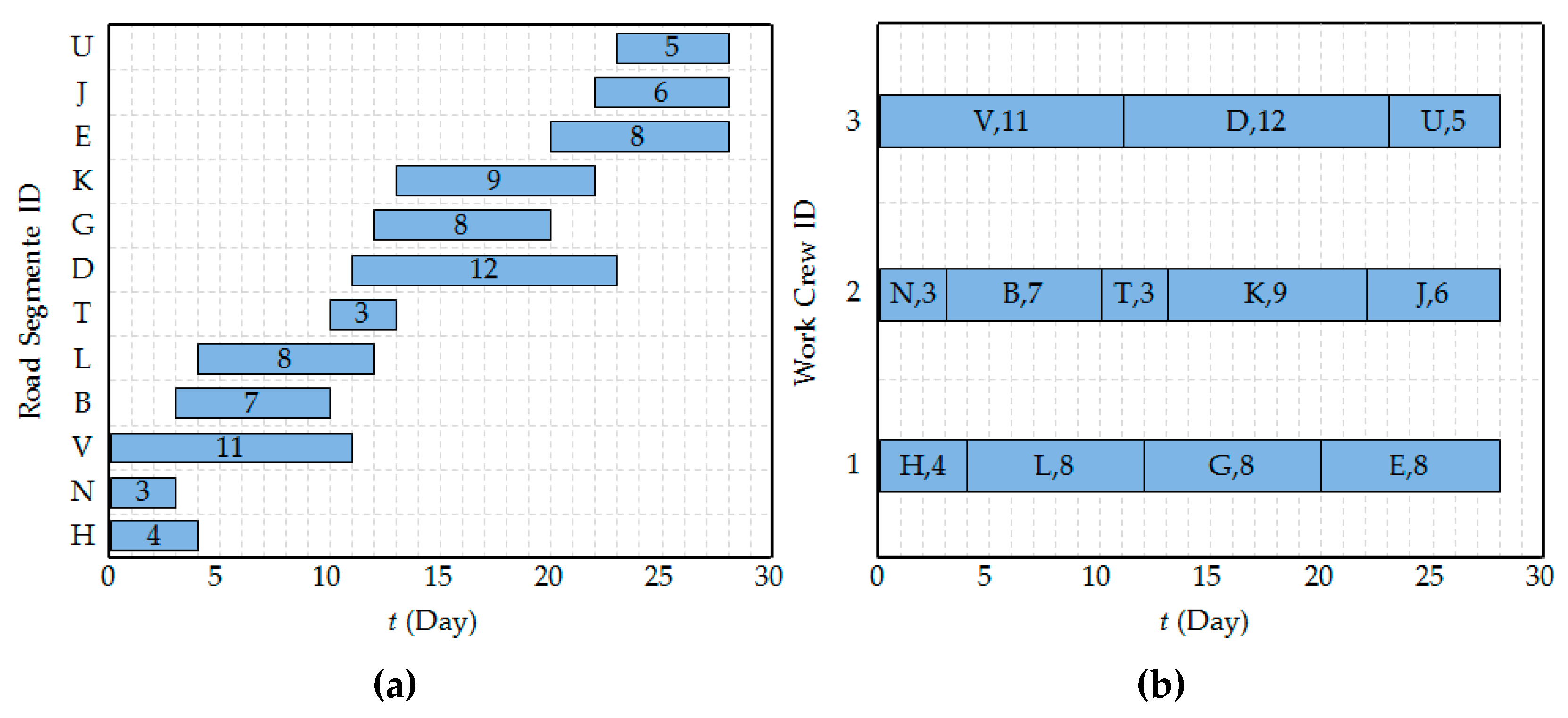
| RR | WC1: V, D, U WC2: N, B, T, K, J WC3: H, L, G, E | WC1: H, T, M, U, K WC2: N, B, F, J, O WC3: I, G, C, P |
| 0.3 | 0.5 | 0.7 | |
|---|---|---|---|
| 0.705 | 0.724 | 0.748 | |
| 0.865 | 0.860 | 0.850 | |
| C | 1870 | 1880 | 1990 |
| M | 27 | 28 | 30 |
| N | 11 | 12 | 12 |
| RR | WC1: M, N, O, P, J WC2: L, I, A WC3: V, C, K | WC1: V, D, U WC2: N, B, T, K, J WC3: H, L, G, E | WC1: D, S, K WC2: N, Q, B, F, J WC3: H, M, V, E |
| 1.5 | 2.0 | 2.5 | |
|---|---|---|---|
| 0.724 | 0.857 | 0.954 | |
| 0.860 | 0.885 | 0.915 | |
| C | 1880 | 1570 | 1270 |
| M | 28 | 23 | 17 |
| N | 12 | 10 | 8 |
| RR | WC1: V, D, U WC2: N, B, T, K, J WC3: H, L, G, E | WC1: V, A, T WC2: N, D, G WC3: H, P, U, K | WC1: Q, V WC2: M, N, B WC3: H, L, U |
| 3 | 5 | 7 | |
|---|---|---|---|
| 0.724 | 0.856 | 0.881 | |
| 0.860 | 0.915 | 0.935 | |
| C | 1880 | 1880 | 1880 |
| M | 28 | 17 | 13 |
| N | 12 | 12 | 12 |
| RR | WC1: V, D, U WC2: N, B, T, K, J WC3: H, L, G, E | WC1: H, N, B, T WC2: D, U WC3: G, E WC4: V, J WC5: L, K | WC1: B, J WC2: D WC3: H, E WC4: G, U WC5: N. K WC6: L, T WC7: V |
| B | 2000 | 2500 | 3000 |
|---|---|---|---|
| 0.724 | 0.867 | 0.867 | |
| 0.860 | 0.820 | 0.820 | |
| C | 1880 | 2410 | 2410 |
| M | 28 | 36 | 36 |
| N | 12 | 15 | 15 |
| RR | WC1: V, D, U WC2: N, B, T, K, J WC3: H, L, G, E | WC1: M, D, G, A WC2: N, B, V, F, E WC3: H, L, U, T, K, J | WC1: M, D, G, A WC2: N, B, V, F, E WC3: H, L, U, T, K, J |
© 2020 by the authors. Licensee MDPI, Basel, Switzerland. This article is an open access article distributed under the terms and conditions of the Creative Commons Attribution (CC BY) license (http://creativecommons.org/licenses/by/4.0/).
Share and Cite
Mao, X.; Lou, X.; Yuan, C.; Zhou, J. Resilience-Based Restoration Model for Supply Chain Networks. Mathematics 2020, 8, 163. https://doi.org/10.3390/math8020163
Mao X, Lou X, Yuan C, Zhou J. Resilience-Based Restoration Model for Supply Chain Networks. Mathematics. 2020; 8(2):163. https://doi.org/10.3390/math8020163
Chicago/Turabian StyleMao, Xinhua, Xin Lou, Changwei Yuan, and Jibiao Zhou. 2020. "Resilience-Based Restoration Model for Supply Chain Networks" Mathematics 8, no. 2: 163. https://doi.org/10.3390/math8020163
APA StyleMao, X., Lou, X., Yuan, C., & Zhou, J. (2020). Resilience-Based Restoration Model for Supply Chain Networks. Mathematics, 8(2), 163. https://doi.org/10.3390/math8020163