Abstract
Cuckoo search (CS) algorithm is a novel swarm intelligence optimization algorithm, which is successfully applied to solve some optimization problems. However, it has some disadvantages, as it is easily trapped in local optimal solutions. Therefore, in this work, a new CS extension with Q-Learning step size and genetic operator, namely dynamic step size cuckoo search algorithm (DMQL-CS), is proposed. Step size control strategy is considered as action in DMQL-CS algorithm, which is used to examine the individual multi-step evolution effect and learn the individual optimal step size by calculating the Q function value. Furthermore, genetic operators are added to DMQL-CS algorithm. Crossover and mutation operations expand search area of the population and improve the diversity of the population. Comparing with various CS algorithms and variants of differential evolution (DE), the results demonstrate that the DMQL-CS algorithm is a competitive swarm algorithm. In addition, the DMQL-CS algorithm was applied to solve the problem of logistics distribution center location. The effectiveness of the proposed method was verified by comparing with cuckoo search (CS), improved cuckoo search algorithm (ICS), modified chaos-enhanced cuckoo search algorithm (CCS), and immune genetic algorithm (IGA) for both 6 and 10 distribution centers.
1. Introduction
Optimization problems have been one of the most important research topics in recent years. They exist in many domains, such as scheduling [1,2], image processing [3,4,5,6], feature selection [7,8,9] and detection [10], path planning [11,12], feature selection [13], cyber-physical social system [14,15], texture discrimination [16], saliency detection [17], classification [18,19], object extraction [20], shape design [21], big data and large-scale optimization [22,23], multi-objective optimization [24], knapsack problem [25,26,27], fault diagnosis [28,29,30], and test-sheet composition [31]. Metaheuristic algorithms [32], a theoretical tool, are based on nature-inspired ideas, which have been extensively used to solve highly non-linear complex multi-objective optimization problems [33,34,35]. Several popular metaheuristics with a stochastic nature are compared in some studies [36,37,38] with deterministic Lipschitz methods by using operational zones. Most of these metaheuristics methods are inspired by natural or physical processes, such as bat algorithm (BA) [39], biogeography-based optimization (BBO) [40], ant colony optimization (ACO) [41], earthworm optimization algorithm (EWA) [42], elephant herding optimization (EHO) [43,44], moth search (MS) algorithm [45], firefly algorithm (FA) [46], artificial bee colony (ABC) [47,48,49], harmony search (HS) [50,51], monarch butterfly optimization (MBO) [52,53], particle swarm optimization (PSO) [54,55], genetic programming [56], krill herd (KH) [57,58,59,60,61,62,63], immune genetic algorithm (IGA) [64], and cuckoo search (CS) [65,66,67,68,69].
Yang and Deb [69] proposed a metaheuristic optimization method named CS algorithm, which is inspired by smart incubation behavior of a type of birds called cuckoos in nature.
CS performs local search well in most cases, but sometimes it cannot escape from local optima, which restricts its ability to carry out full search globally. To enhance the ability of CS, Mlakar et al. [70] proposed a novel hybrid self-adaptively CS algorithm adding three features: a self-adaptively of cuckoo search control parameters, a linear population reduction, and a balancing of the exploration search strategies. Li et al. [71] enhanced the exploitation ability of the cuckoo search algorithm by using an orthogonal learning strategy. An improved discrete version of CS was presented by Ouaarab et al. [72].
On the other hand, most researchers agree that the performance of algorithms can be improved by using learning techniques. For example, Wang et al. [73] presented a new method to enhance learning speed and improved final performance, which directly tuned the Q-values to affect the action selection policy. Alex et al. [74] presented a new evolutionary cooperative learning scheme that is able to solve function approximation and classification problems, improving accuracy and generalization capabilities. A new CS algorithm named snap-drift cuckoo search (SDCS) was presented by Hojjat et al. [75]. In SDCS, a snap-drift learning strategy is employed to improve search operators. The snap-drift learning strategy provides an online trade-off between local and global search via two snap and drift modes.
Although much effort has been made to enhance the performance of CS, many of the variants fail to improve the performance of CS algorithm on certain complicated problems. Furthermore, there are few studies on optimizing the parameters of CS algorithm by using learning strategy. In this paper, we present an improved CS algorithm called dynamic step size cuckoo search algorithm (DMQL-CS) that adopts strategies with Q-Learning and genetic operator. Step size strategy of the traditional CS focused only on examining the individual fitness value based on the one-step evolution effect of individual, but ignored the evaluation of step size from the multi-step evolution effect, which is not conducive to the evolution of the algorithm. We use Q-Learning method to optimize the step size, in which the most appropriate step size control strategies are retained for the next generation. At the same time, their weights are adaptively adjusted by using learning rate, which is used to guide individuals to search for a better solution at the next evolution. In addition, crossover operation and mutation operation are added into the DMQL-CS algorithm to accelerate the convergence speed of the algorithm and expand the diversity of the population.
The present manuscript differs from other similar work insofar as the advantage of learning based on Q-Learning and genetic operators. Q-Learning considers the multi-step evolution effect of individual such that the most appropriate step size control strategies are retained for the next generation. For the proposed DMQL-CS approach, the outstanding work of the paper is mainly listed in the following two aspects:
- (1)
- In the DMQL-CS algorithm, the step size strategy is considered as an action which applies multiple step control strategies (linear decreasing strategy, non-linear decreasing strategy, and adaptively step-size strategy). In the DMQL-CS algorithm, according to multi-step effect of individual for a few steps forward, the optimal step size control strategy is learned. During each learning evolution step size, finally, the optimal individual and corresponding optimal step size strategy are derived by calculating the Q function value. The current individual continues to evolve through the step size obtained, which increases the adaptability of individual evolution.
- (2)
- The research introduces two genetic operators, crossover and mutation, into the DMQL-CS algorithm, intended for accelerating convergence. During crossover and mutation process, chromosomes are divided into pairs according to certain probability. We introduce the specifically designed crossover operation into problem of logistics distribution center location in this paper, which determines the performance of the algorithm to some extent. To improve the search ability of the CS algorithm, numerous strategies have been designed to adjust the crossover rate. In this work, a self-adaptive scheme is used to adjust the crossover rate. Genetic operators expand the search area of the population to improve the exploration and maintain the diversity of the population, which also helps to improve the exploration of the population of learners.
Finally, the DMQL-CS method was tested on 15 benchmark functions, CEC 2013 test suite, and the problem of logistics distribution center location. The experimental results compared with those of other approaches demonstrated the superiority of the proposed strategy. A series of simulation experiments showed that DMQL-CS performs more accurately and efficiently than other evolutionary methods in terms of the quality of the solution and convergence rate.
The remainder of this paper is organized as follows. In Section 2, the related work on cuckoo search is presented. Section 3 presents cuckoo search. The proposed DMQL-CS algorithm, including Q-Learning model, step size control model with Q-Learning, and genetic operator, is described in Section 4. The comparison with other methods, through 15 functions, CEC 2013 test suite, and the problem of logistics distribution center location, is given in Section 5. Finally, Section 6 concludes this paper and points out some future research directions.
2. Related Work
CS algorithm is capable of finding the best solutions by continuously using new and potentially better solution to replace a not-so-good cuckoo in the population, and it has been applied successfully to diverse fields. Recently, many CS variants have been developed to improve the performance of the CS algorithm. These variants can be generally divided into four categories: (1) parameter control [70]; (2) novel learning schemes [76]; (3) hybrid methods with other algorithm [74]; and (4) local search operator [77].
Due to the important influence of control parameters for the performance, much meaningful work has been done on the control parameter settings of CS algorithm. Initially, step size parameter control was investigated to improve the performance of CS algorithms. For instance, aiming at the faults that Cuckoo Search algorithm cannot acquire exact solutions and converges slowly in the later period, Ma et al. [78] proposed a self-adaptively step size adjustment cuckoo search algorithm (ASCS), which is an adaptively adjusted step size by using the distance between cuckoo nest location and the optimal nest location, which speeds up CS algorithm speed and improves the calculation accuracy. To balance the exploration and exploitation, Li and Yin [79] introduced two mutation rules and combined these two rules using a linear decreasing probability. Then, an adaptive parameter adjustment strategy was developed according to the relative success number of two newly added parameters in the previous iteration. Comparison results of the proposed algorithm show that this scheme is better than other algorithms. Two important factors, speed factor and aggregation factor, were defined by Yang et al. [80]. Then, according to these two factors, the step size and discovery probability were regulated. Experimental results show that the CS with improved step size and discovery probability has strong competitiveness in tackling numerical optimization problems. Li et al. [79] proposed the self-adaptive parameter CS algorithm, which uses two new mutation rules based on the rand and best individuals among the entire population. The self-adaptive parameter is set as a uniform random value based on the relative success number of the two new proposed parameters in the previous period, which enhance diversity of the population. Experimental results show that the proposed method performs better than twelve algorithms from the literature.
Li et al. [65] proposed an enhanced CS algorithm called dynamic CS with Taguchi opposition-based search and dynamic evaluation. The Taguchi search strategy provided random generalized learning based on opposing relationships to enhance the exploration ability of the algorithm. The dynamic evaluation strategy reduced the number of function evaluations, and accelerated the convergence property. Statistical comparisons of experimental results showed that the proposed algorithm makes an appropriate trade-off between exploration and exploitation. Li et al. [81] proposed a new cuckoo search algorithm extension based on self-adaptive knowledge learning, in which a learning model with individual history knowledge and population knowledge is introduced into the CS algorithm. Individuals constantly adjust their position according to historical knowledge and communicate in the optimization process. Statistical comparisons of the experimental results showed that the proposed algorithm is a competitive new type of algorithm. Hojjat et al. [75] presented a new CS algorithm, called snap-drift cuckoo search (SDCS), which first employs a learning strategy and then considers improved search operators. The snap-drift learning strategy provides an online trade-off between local and global search via two snap and drift modes. SDCS tends to increase global search to prevent algorithm of being trapped in local minima via snap mode and reinforces the local search to enhance the convergence rate via drift mode. Statistical comparisons of experimental results showed that SDCS is superior to modified CS algorithms in terms of convergence speed and robustness.
According to the rand and best individuals among the entire population, Cheng et al. [82] proposed an ensemble CS variant in which three different cuckoo search algorithms coexist in the entire search process, which compete to produce better offspring for numerical optimization. Then, an external archive is introduced to further maintain population diversity. Statistical comparisons of experimental results showed that the improved CS variant is superior to modified CS algorithms in terms of convergence speed and robustness. Wen et al. [83] proposed a new hybrid algorithm based on grey wolf optimizer and cuckoo search (GWOCS), which was developed to extract the parameters of different PV cell models with the experimental data under different operating conditions. Zhang et al. [84] proposed an ensemble CS variant that divides the population into two subgroups and adopts CS and DE for these two subgroups independently. These two subgroups can exchange useful information by division. These two algorithms can utilize each other’s advantages to complement their shortcomings, thus balancing the quality of solution and the computation consumption. Zhang et al. [85] devised a hybridization of CS and covariance matrix adaption evolution strategy (CMA_ES) to improve performance for the different optimization problems. Computational results demonstrate that the proposed algorithm outperforms other competitor algorithms. Tang et al. [86] introduced Gaussian distribution, Cauchy distribution, Levy distribution, and Uniform distribution, improving the performance of cuckoo search algorithm by the method of pair combination. Simulation results show that the hybrid distribution with Cauchy distribution and Levy distribution can make the CS algorithm perform better.
With respect to applications, CS has been extensively applied to many domains, such as neural networks [87], image processing [88], nonlinear systems [89,90], network structural optimization [91], agriculture optimization [92], engineering optimization [93], and scheduling [94]. These applications indicate that CS algorithm is an effective and efficient optimizer for solving some real-world problems.
3. Cuckoo Search
The cuckoo search algorithm [69] is a stochastic optimization algorithm that models brood parasitism of cuckoo birds. The algorithm is based on the obligate brood parasitic behavior found in some cuckoo nests by combining a model of this behavior with the principles of Lévy flights, which discard worst solutions and generate new ones after some certain iteration.
According to the mentioned characteristics, CS can be expressed as three idealized rules:
- (1)
- Each cuckoo lays one egg at a time, and places it in a randomly chosen nest.
- (2)
- The best nests with the highest-quality eggs (solutions) will be carried over to the next generations.
- (3)
- The number of available host nests is fixed, and the alien egg is discovered by the host bird with the probability . If the alien egg is discovered, the nest is abandoned and a new nest is built in a new location.
The CS algorithm is equiponderant to the integration of Lévy flights. The position of the ith nest is indicated by using D-dimensional vector ; a Lévy flight is performed:
where α > 0 is the step size that is used to control the range of the random search, which should be related to the scales of the problem of interests, and step size information is more useful can be computed by Equation (2). The product means entry-wise multiplications. and are two different solutions selected randomly. A new solution with the same number of cuckoos is generated after partial solutions are discarded. with the random walk can be expressed in terms of a simple power-law equation.
where μ and t are two random numbers following the normal distribution and β often takes a fixed value of 1.5.
where Γ is gamma function. μ and v are random numbers drawn from a normal distribution with mean of 0 and standard deviation of 1, which have an infinite variance with an infinite mean. Here, the consecutive jumps/steps of a cuckoo essentially form a random walk process that obeys a power-law step length distribution with a heavy tail. In Lévy flights random walk component, the new solution Xi is generated through Equation (6).
where Xg,best represents the best solution obtained thus far and α0 is a scaling factor. The Lévy distribution is a process of random walk; after a series of smaller steps, Lévy flights can suddenly obtain a relatively larger step size. Lévy distribution is implemented at the initial stage of algorithm, which helps to jump out of the local optimum.
where and are random solutions at the tth generation. r generates a random number between −1 and 1. The basic steps of the CS algorithm are summarized in Algorithm 1.
| Algorithm 1 CS Algorithm. |
| (1) randomly initialize population of n host nests |
| (2) calculate fitness value for each solution in each nest |
| (3) while (stopping criterion is not meet do) |
| (4) Generate as new solution by using Lévy flights; |
| (5) Choose candidate solution ; |
| (6) if |
| (7) Replace with new solution ; |
| (8) end if |
| (9) Throw out a fraction (pa) of worst nests; |
| (10) Generate solution using Equation (3); |
| (11) if |
| (12) Replace with new solution ; |
| (13) end if |
| (14) Rank the solution and find the current best. |
| (15) end while |
4. Cuckoo Search Algorithm with Q-Learning and Genetic Operations
4.1. Q-Learning Model
Q-Learning model, a milestone in reinforcement learning research, is an enhanced learning method that is not constrained by the problem model. The optimal policy of Q-Learning is generated by executing the action with the highest expected Q-values, which is the action of maximizing the cumulative benefits with a discount. Control strategy of the optimal step size can be transformed into the optimal action for the agent. The Q function is defined as discounted. In general, the environment is the current state in which the agent makes decisions. The agent includes a set of feasible actions which affect both next state and reward. In fact, the Q-Learning is a mapping from state–action to prediction. The output for state vector s and action a are denoted by Q-value :
where represents the cumulative reward of action in the state of s at time t. indicates the cumulative reward of action in the state vector s at time t + 1. is the reward received for the action a at time t + 1. When is terminal, goes to zero, where a and represent learning factors and discount factors, respectively (, ). determines the impact of lagging returns on optimal action. Q-Learning provides strong proof of convergence. The Q value will converge with probability 1 to Q when each state–action pair is repeatedly visited. The error of Q (s, a) must be reduced by whenever it is updated. When each state–action pair is visited infinitely, the estimates of converge to real values of as .
4.2. Step Size Control Model by Using Q-Learning
In CS algorithm, the most important parameter is step size scaling factor with the typical characteristics of Lévy flight, in addition to the population size, the number of iterations, and the probability of discovery. Step size scaling factor is as suitable action that is selected to control an individual search process. The accuracy of selected parameter can be improved by predicting before making an action decision. When an individual selects an action, the advantages and disadvantages of various actions can be evaluated by the multi-step effect of individual. Q-Learning is helpful to learn the optimal step size control strategy and transform optimal step size control strategy into optimal action selected of agent.
During the iteration of CS algorithm, the fixed step size strategy cannot meet the dynamic requirements of the algorithm. Considering the aforementioned facts, at the later stage of the CS algorithm, we add three step size control methods in the iterative process: (1) Dynamic linear decreasing strategy (L1) is defined by Equation (9). (2) Dynamic non-linear decreasing strategy (L2) is defined by Equation (10). (3) Adaptive step-size strategy (L3) is defined by Equation (11). Each individual obtains the optimal step size control strategy via learning multiple steps forward, thus becomes close to the optimal solution. Therefore, we try to evaluate the step size control strategy by using multi-step evolution method, which increases the adaptability of individual evolution and improves the performance of the algorithm. The current best step size control strategy is selected to execute the next iteration by using Q-Learning method.
where tmax expresses the total number of iterations, t is the current number of iterations, and dmax is the maximum distance between the optimal nest and all other nests. , is the initial value of step size.
In Q-Learning algorithm, the agent receives feedback, which is called reward, for each action. When the state is set to s and the action is set to a, a set of actions is set to , the agent has n actions to choose from each state, and the maximum reward of discount for the agent is:
where is the immediate benefits for state s. is the maximum return value that the agent select different actions at the next state . is the action which is selected at the next state . is the discount factor. The benefits that the agent selecting action a receives is:
where m represents the number of steps forward, . When = 0, Q is reduced to one step forward. When is close to 1, the lagging benefits of optimal action increase gradually. is the immediate benefit that the agent selects action a, which expresses that individuals have evolved once, and new individuals use to generate new individuals again. At this time, the benefit is recorded as . By analogy, after m evolution, a new individual is generated by using , and the corresponding benefit is recorded as .
n offspring will be generated after each evolution. These offspring are evolved again by adopting n strategies. offspring will be produced after m evolutions. Boltzmann distribution is used to calculate the probability of new individuals retained. Boltzmann distribution can be defined by Equation (15):
where indicates the immediate benefits of the ith step strategy and represents the temperature.
The step size control strategy corresponding to the maximum probability is selected. The results of each generation are simplified by Boltzmann distribution. is defined as the fitness function corresponding to parent individual in the population and is the fitness function corresponding to the individual after adopting the parameter selection strategy. Substituting into Equation (13) Equation (16) is obtained.
where , ; according to Equation (17), it can be concluded that , . The step size control strategy model with Q-Learning is described in Algorithm 2 and Figure 1.
| Algorithm 2 Step size with Q-Learning. |
| (1) Each individual is expressed as (x, σ), and the number of learning steps M is set; |
| (2) Generate three new offspring for each individual by using the given step size control strategy (Linear decreasing strategy, non-linear decreasing strategy, adaptively step-size dynamic adjustment strategy), and set t = 1; |
| (3) Do while t < m |
| Each individual generates three offspring by using the given step size control strategy, as shown in Equations (9)–(12). |
| Calculate the probability of the newly generated offspring by using the Boltzmann distribution, and an individual is selected according to the probability. |
| t = t + 1; |
| (4) Calculate the corresponding Q value of each retained individual according to the three-step selection strategy. The step size corresponding to the step control strategy is retained when Q is maximized, the corresponding offspring are selected, and other offspring will be discarded. |
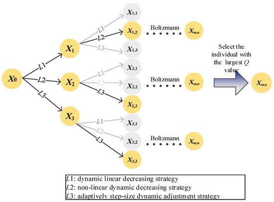
Figure 1.
Step selection model with Q-Learning.
4.3. Genetic Operation
4.3.1. Crossover Process
As we know, two of the most important operators are the crossover operator and mutation operator for genetic operation [95], which have a great influence on the behavior and performance of genetic operation. Therefore, these operations are introduced into the DMQL-CS algorithm. In crossover process, a parameter Cr is defined as the probability of crossover and chromosomes are divided into pairs. We introduce the specifically designed crossover operation into the problem of logistics distribution center location in this paper, and apply it to a pair of chromosomes G1 and G2, as illustrated in Figure 2. First, some genes are randomly selected in chromosome G1, as those pointed to by a red arrow in the illustration. Then, these genes are found in chromosome G2, as pointed to by a green arrow. If the same gene is not found in G2, two genes are randomly selected as the crossover point. Generate one child as the combination of red-pointed genes in G1 and the rest of blue genes in G2, and generate another child as the combination of green-pointed genes in G2 and the rest of blue genes in G1. Finally, the optimal is found as an arc between any two nodes by using enumeration method, which keep the child to obtain the lowest objective value, and obtain chromosomes R1 and R2. Two chromosomes are selected from the parents and children with the smallest objective values to replace the parents.
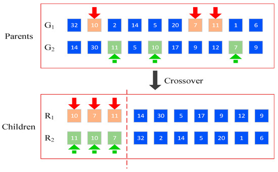
Figure 2.
Crossover process of chromosomes.
At the same time, the crossover rate (Cr) is a critical factor for how the crossover operator behaves, which determines the performance of the algorithm to some extent. To improve the search ability of the algorithm, a substantial number of strategies have been designed to adjust the crossover rate. In this work, a self-adaptive scheme was used to adjust the crossover rate, which can be calculated as shown below.
where , is the average fitness, is the max fitness, and is the scale factor between 0 and 1, = 0.02.
4.3.2. Mutation Process
A parameter Cm is defined as the mutation probability. The number r is randomly generated in the interval [0, 1]. If r < Cm, the ith chromosome G1 is selected to perform the mutation operation and this process is repeated at each iteration. For illustration, we continue to use the problem of logistics distribution center location with 40 cities and 10 distribution centers. Two genes located on chromosome G1 are randomly selected and their positions swapped to obtain a possible child. Then, the optimal is found as an arc between any two nodes by using enumeration method, which keeps the child obtaining the lowest objective value. Finally, we get chromosome R1, as shown in Figure 3. If R1 has a smaller objective value than G1, G1 is replaced with R1, else G1 is retained. A new generation of population is generated after the evaluation, crossover, and mutation operations.
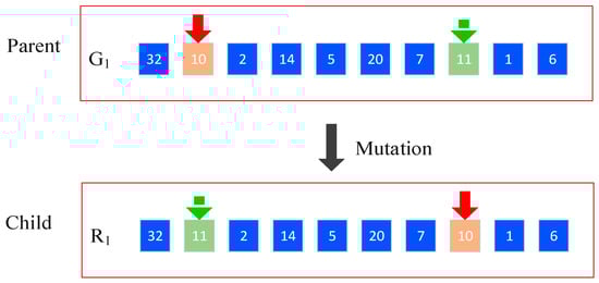
Figure 3.
Mutation process of chromosomes.
4.3.3. Cuckoo Search Algorithm with Q-Learning Model and Genetic Operator
Introducing Q-Learning into CS algorithm helps to learn the optimal step size strategy and transform. Crossover and mutation strategies enable the nest to approach the historical optimal nest quickly, which can speed up the global convergence rate. The structure of the genetic operator cuckoo search algorithm with Q-Learning model (DMQL-CS) is described in Algorithm 3.
| Algorithm 3 DMQL-CS Algorithm. |
| Input: Population size, NP; Maximum number of function evaluations, MAX_FES, LP |
| (1) Randomly initialize position of NP nest, FES = NP; |
| (2) Calculate the fitness value of each initial solution; |
| (3) while (stopping criterion is not meet do) |
| (4) Select the best step size control strategy according to Algorithm 2; |
| (5) Generate new solution with the new step size by Lévy flights; |
| (6) Randomly choose a candidate solution ; |
| (7) if |
| (8) Replace with new solution ; |
| (9) end if |
| (10) Generate new solution by using crossover operator and mutation operator; |
| (11) Throw out a fraction (pa) of worst nests, generate solution using Equation (3); |
| (12) if |
| (13) Replace with new solution ; |
| (14) end if |
| (15) Rank the solution and find the current best. |
| (16) end while |
4.3.4. Analysis of Algorithm Complexity
To show the convergence effect of the algorithm, typical function Rastrigrin was selected to analyze the convergent process of DMQL-CS algorithm. Figure 4 shows the location distribution of cuckoo individuals in the search area with a population size of 10. Figure 4a describes the individual distribution at the first generation, Figure 4b describes the individual distribution at the 30th generation, Figure 4c describes the individual distribution at the 50th generation, and Figure 4d describes the individual distribution at the 80th generation. In Figure 4, it can be seen that the activity area of individuals keeps changing and gradually draws closer to the optimal solution during the evolution of the algorithm. It is worth noting that algorithm converged at the 80th generation, which indicates that Q-learning and genetic operation expand activity area of the population and improve the convergence performance of the DMQL-CS algorithm.
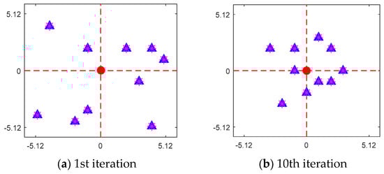
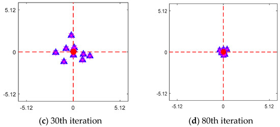
Figure 4.
Analysis of algorithm complexity.
5. Results
5.1. Optimization of Functions and Parameter Settings
In this section, to check and verify the efficacy DMQL-CS algorithm, it is thoroughly investigated through benchmark evaluations from various respects. We tested our algorithms on two function groups: Group A and Group B. Group A contains fourteen different global optimization problems, as shown in Table 1. Group B is the CEC 2013 test suite including 28 benchmark functions. To make a fair comparison, all experiments were carried out on a P4 Dual-core platform with a 1.75 GHz processor and 4 GB memory, running under the Windows 7.0 operating system. The algorithms were written in MATLAB R2017a. The following were set: maximum number of evaluation MAX_FES = NP × 105, population size NP = 30, run time T = 30, and probability of foreign eggs pa = 0.25.

Table 1.
Brief description of fifteen functions.
5.2. Comparison with Other CS Variants and Rank Based Analysis
We compared the performance of DMQL-CS with four improved CS variants: CCS [68], GCS [96], CSPSO [97], and OLCS [71]. CCS is a modified Chaos enhanced Cuckoo search algorithm. GCS introduces Gaussian disturbance into the CS algorithm. CSPSO is a kind of algorithm combining CS with PSO. A new search strategy based on orthogonal learning strategy is used in OLCS to enhance the exploitation ability of CS algorithm. The parameter configurations of these algorithms are shown in Table 2 according to corresponding references. Fifteen benchmark functions are shown in Table 3, Table 4, Table 5 and Table 6 at D = 30 and D = 50. All optimization algorithms were tested by using the same parameter settings: population size NP = 30, MAX_FES = 100,000 × D, probability switching parameter pa = 0.25, and run time T = 30.
Table 2.
The personal parameters of different algorithms.
Table 3.
The optimization results obtained by CCS, GCS, CSPSO, OLCS, and DMQL-CS at D = 30.
Table 4.
The ranking of different strategies according to the Friedman test.
Table 5.
The optimization results obtained by CCS, GCS, CSPSO, OLCS, and DMQL-CS at D = 50.
Table 6.
The ranking of different strategies according to the Friedman test.
As shown in Table 3, the DMQL-CS find global optima 0.00 on the four benchmark functions F1, F6, F7, and F14 when D = 30. For unimodal functions F1–F5, the DMQL-CS algorithm achieves higher accuracy than other CS variants on functions F2, F4, and F5. DMQL-CS is only inferior to OLCS on F2. For multimodal problems F6–F11, DMQL-CS algorithm shows higher performance than the other CS variants on functions F6, F7, F8, and F11. For F10, the same solution is found by the four algorithms (CCS, GCS, CSPSO, and OLCS). For the shifted unimodal functions F13–F15, DMQL-CS is significantly better than CCS, GCS, OLCS, and CSPSO on F13, F14 and F15. For F12, CCS performs the best.
DMQL-CS still has outstanding optimization performance when D = 50, as shown in Table 5. From the results, it is apparent that the convergence precision of other algorithms drops rapidly, while the DMQL-CS algorithm achieves better performance than other CS variants on most functions. DMQL-CS and OLCS achieve the global optimum on function F7. DMQL-CS cannot get the minimum; even then, it is not inferior to other algorithms on F4, F5, F10, F12, F13, and F15. In addition, the DMQL-CS demonstrates a remarkable accuracy on benchmark F1 and F2. Comparing with the optimization results, we can conclude that the DMQL-CS optimization algorithm explored a larger search space than other CS variants. Moreover, it is important to point out that, regardless of the problem’s dimensionality, the DMQL-CS converges to the better solution on the shifted multimodal functions F13, F14 and F15. Therefore, these statistical tests confirmed that DMQL-CS algorithm with Q-Learning step size and genetic operators has a better overall performance than all other tested competitors. For a clearer observation that DMQL-CS performs best, Table 4 shows the ranking of the strategies in Table 3 according to the Friedman test. We can see that DMQL-CS obtains the best rank, OLCS ranks second, followed by CCS, GCS, and CSPSO. Table 6 shows the ranking of the five strategies according to the Friedman test. OLCS obtains the best rank, DMQL-CS ranks second, followed by GCS, CSPSO, and CCS.
To further demonstrate the convergence of DMQL-CS, the median convergence properties of five algorithms are illustrated in Figure 5. There is no obvious “evolution stagnation” for all algorithms. For the same population size and number of generations, the optimization performance of the four algorithms declines rapidly. However, DMQL-CS can get better convergence curve than CCS, GCS, CSPSO, and OLCS on F1–F2, F5–F6, F12, and F14. In Figure 5, DMQL-CS algorithm converged to the specified error threshold on function F1, which suggests that DMQL-CS algorithm has a faster convergence rate for the specified error threshold. Generally speaking, when M is too small, useful step size information will not be learned. When M is too large, the speed of Q-Learning will be slowed down. When the value of M is 3 or 5, the convergence performance of DMQL-CS can be improved for the ill-condition function F2, complex multimodal functions F5–F6, and Shifted multimodal functions F12 and F14. It is worth mentioning that the accuracy of OLCS is similar to that of DMQL-CS, but the convergence speed of DMQL-CS is much faster than that of OLCS. For multimodal function, all algorithms converge to the specified error threshold with the same number of successes. However, DMQL-CS has good reliability, stability, and faster convergence rate on functions F5–F6. For function F14, DMQL-CS algorithms can find the global optimum with 50,000 FES. As mentioned above, it can be clearly observed that DMQL-CS provided better performance than the four other CS versions, and achieves a promising solution on most test functions.
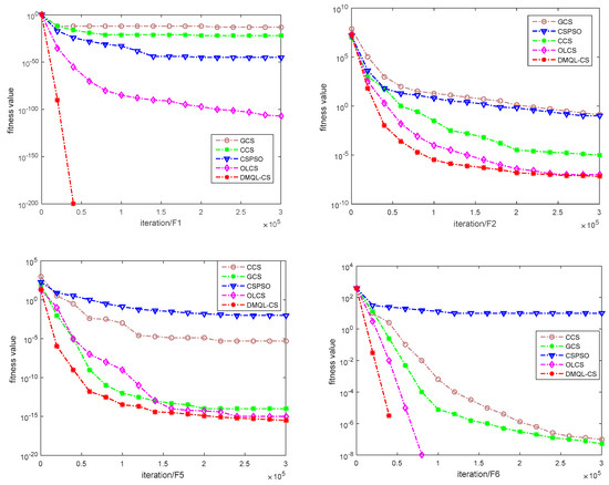
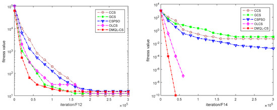
Figure 5.
Convergence curves of different algorithms on test functions when D = 30.
A series of comparisons proved the high efficiency of DMQL-CS. The performance ranking of the multiple algorithms of the test suite is listed in Table 7, Table 8 and Table 9. The average rankings of the five CS variants for functions F1–F8 are shown in Table 7 (D = 30 and D = 50). The average rankings of the five CS variants for functions F9–F15 are shown in Table 8 (D = 30 and D = 50). In competition ranking, if performances of algorithms are the same, they received the same rank. It can be seen in Table 7, Table 8 and Table 9 that the average ranking value of DMQL-CS on D = 30 is smaller than that of CCS, GCS, OLCS, and CSPSO. Therefore, the performance of DMQL-CS is better than the other CS variants. When D = 50, the results are similar to those when D = 30, with the average ranking value of DMQL-CS being smaller than those of CCS, GCS, OLCS, and CSPSO.
Table 7.
Rank results of each algorithm on F1–F8 for D = 30 and D = 50.
Table 8.
Rank results of each algorithm on F9-F15 for D = 30 and D = 50.
Table 9.
Total rank and final rank on F1–F15 for D = 30 and D = 50.
In Table 9, DMQL-CS has the best total rank when D = 30 and D = 50, i.e., 25 and 29, which means that DMQL-CS has the best performance on most of the test functions compared with other algorithms. OLCS has the second-best total rank at D = 30 and D = 50, i.e., 29 and 30. Obviously, OLCS has better performance than the three other algorithms on high-dimension test functions. Similarly, in Table 9, the order can be clearly observed: DMQL-CS > OLCS > CCS > GCS > CSPSO at D = 30; and DMQL-CS > OLCS > GCS > CCS > CSPSO at D = 50. Based on the analysis of the above, DMQL-CS has the best performance among all the algorithms on both D = 30 and D = 50.
5.3. Statistical Analysis of Performance for the CEC 2013 Test Suite
In this section, the CEC 2013 test suite is selected to test the effectiveness of three different algorithms (jDE [98], SaDE [99], and CLPSO [100]). These algorithms can be seen as representatives of the state-of-the-art algorithms for comparison, and the parameter configurations of these algorithms were set according to the corresponding references, as listed in Table 10.
Table 10.
The personal parameters of different algorithms.
Table 11 summarizes the results of CEC 2013 test problems on 28 benchmark functions for 30-dimensional case. The rank was used to obtain the ranking of different algorithms on all problems, as shown in Table 12. This means that DMQL-CS gets the first rank and outperforms jDE, SaDE, and CLPSO. The results in Table 11 indicate that with 80% certainty DMQL-CS has statistically higher accuracy than the other algorithms. Note that DMQL-CS obtains the global optimal value 0.00 on F1 and F11. DMQL-CS is significantly better than the three other algorithms, especially on functions CEC 2013-F1, CEC 2013-F2, and CEC 2013-F4. About basic Multimodal Function and composition Functions (CEC 2013-F6–CEC 2013-F28), the ability of DMQL-CS to find the optimal solution is slightly better than that of CLPSO. For functions CEC 2013-F5, CEC 2013-F7, CEC 2013-F17, CEC 2013-F22, and CEC 2013-F25, the performance of DMQL-CS is slightly worse than the other algorithms. For the Unimodal problem CEC 2013-F3, jDE obtains the best solution 2.99 × 10⁶. On Shift Rastrigin Function, SaDE and jDE can get better solutions of 1.10 × 101 and 1.06 × 10⁻⁴, respectively. For CEC 2013-F25–CEC 2013-F26, DMQL-CS is obviously better than SaDE and jDE. CLPSO has the weakest ability to find the optimal solution for 28 functions. From the above results, it can be seen that DMQL-CS with Q-Learning and genetic operations has a better overall performance than all other tested competitors on the CEC 2013 test suite. Table 13 reports the rankings of the results between DMQL-CS and other algorithms. In Table 13, it can be seen that DMQL-CS performs the best among the four algorithms. DMQL-CS exhibits consistent ranks of the first in optimizing most of the functions. For a clearer observation that DMQL-CS performs best, Table 12 shows the ranking of the algorithms in according to the Friedman test. DMQL-CS obtains the best rank, jDE ranks second, followed by SaDE and CLPSO.
Table 11.
The mean and standard deviation (STD) of CEC 2013 test suite with four algorithms.
Table 12.
The ranking of different strategies according to the Friedman test.
Table 13.
Comparisons between DMQL-CS and other algorithms for CEC 2013 test suite.
5.4. Application in the Problem of Logistics Distribution Center Location
5.4.1. Problem Description
The location of logistics distribution center is an important link in the logistics system. The location of distribution center determines the efficiency of the entire logistics network system and the utilization of resources. The location selection model of logistics distribution center is a nonlinear model with more complex constraints and non-smooth characteristics, which can be attributed to HP-hard problem. The problem of logistics distribution center location can be described as: m cargo distribution centers are searched in n demand points, so that the distance between m searched distribution centers and other n cargo demand points is the shortest. At the same time, the following constraint conditions must be met: the supply of goods in the distribution center can meet the requirements of the cargo demand points; the goods required for a cargo demand point can only be provided by one distribution center; and the cost of transporting the goods to the distribution center is not considered. According to the above assumptions, the mathematical model of the problem for logistics distribution center location can be described as:
where Equation (18) is the objective function, cost represents the transportation cost, m is the number of logistics distribution center, n determines the number of goods demand point, nestj is the demand quantity of demand point j, and disti,j indicates the distance between distribution center i and goods demand point j. When ui,j is equal to 1, the goods of demand point j are distributed by distribution point i. Equations (19)–(24) are the constraints. Equation (19) defines that a demand point of goods can only be distributed by a distribution center. Equation (20) indicates that each demand point of goods must have a distribution center to distribute goods. Equation (21) represents the number of goods demand points for a distribution center. Equations (22)–(24) are the relevant definitions.
5.4.2. Analysis of Experimental Results
To verify the performance of the DMQL-CS algorithm in solving the problem of logistics distribution center location, 40 demand points were adopted. The geographical position coordinates and demands are shown in Table 14. To make a fair comparison, all experiments were carried out on a P4 Dual-core platform with a 1.75 GHz processor and 4 GB memory, running under the Windows 7.0 operating system. The algorithms were written by MATLAB R2017a. The maximum number of iterations, population size, and the times of running were set to 30,000, 15, and 30, respectively. The probability of foreign eggs being found was = 0.25.
Table 14.
The geographical position coordinates and demands.
To further verify the efficiency of the DMQL-CS algorithm, the effectiveness of the proposed method was verified by comparing the standard cuckoo search algorithm (CS) [69], the improved cuckoo search algorithm (ICS) [101], a modified chaos-enhanced cuckoo search algorithm (CCS) [68], and the immune genetic algorithm (IGA) [64]. Figure 5 shows the average convergence curve and optimal convergence curve of DMQL-CS algorithm for running 20, 30, and 50 times, respectively, in 40 cities and six distribution centers. The six optimal distribution center points and optimal routes found by DMQL-CS algorithm are also shown in Figure 6. Figure 7 shows the average convergence curve and optimal convergence curve of DMQL-CS algorithm running 20, 30, and 50 times, respectively, in 40 cities and 10 distribution centers. Table 15 shows distribution ranges for six distribution centers in 40 cities, and Table 16 shows distribution ranges for 10 distribution centers in 40 cities.

Figure 6.
Convergence curves and optimal distribution centers scheme for the DMQL-CS algorithm in 6 distribution centers.
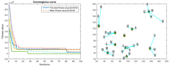
Figure 7.
Convergence curves and optimal distribution centers scheme for the DMQL-CS algorithm in 10 distribution centers.
Table 15.
The distribution scheme for six distribution centers in 40 cities.
Table 16.
The distribution scheme for 10 distribution centers in 40 cities.
For the first set of experiments, the DMQL-CS algorithm was run 20, 30, and 50 times independently in 40 cities for six distribution centers. As shown in Figure 6, the average convergence curve can converge at 30 iterations. It indicates that the fitness value decreases rapidly for the logistics distribution center location method based on DMQL-CS algorithm at early stage of the algorithm. The optimal distribution cost and average distribution cost obtained by the DMQL-CS algorithm are 4.5013 × 10⁴ and 4.8060 × 10⁴, respectively, which indicates that DMQL-CS has high solution accuracy for six distribution centers and reduces the cost of logistics distribution. The optimal distribution center points found in Figure 3 are: 10, 21, 20, 22, 1, and 15.
For the second set of experiments, the DMQL-CS algorithm was run 20, 30, and 50 times independently for 40 cities and 10 distribution centers. As shown in Figure 7, the average convergence curve can converge at 20 iterations. The optimal distribution cost and average distribution cost obtained by the DMQL-CS algorithm are 2.9811 × 10⁴ and 3.0157 × 10⁴, respectively, which indicates that DMQL-CS has high solution accuracy not only for six distribution centers but also for 10 distribution centers. The 10 optimal distribution centers and distribution addressing schemes are shown in Table 16 and Figure 7. The optimal distribution center points are: 30, 23, 14, 18, 11, 28, 21, 1, 20, and 15.
Due to limited space, only three comparison algorithms (CS [69], CCS [68], and IGA [64]) are listed in this paper. IGA algorithm introduced crossover and variation strategy into immune algorithm, which improves performance of the immune algorithm. In this experiment, the convergence curves and optimal distribution scheme diagrams of 6 and 10 distribution centers in 40 cities are shown, respectively. Figure 8 and Figure 9 show the convergence curves and optimal distribution centers scheme for the IGA algorithm for 6 and 10 distribution centers. Figure 10 and Figure 11 show the convergence curves and optimal distribution centers scheme for the CS algorithm for 6 and 10 distribution centers. Figure 12 and Figure 13 show the convergence curves and optimal distribution centers scheme for CCS algorithm for 6 and 10 distribution centers. The six optimal distribution centers and distribution addressing schemes for these algorithms are shown in Table 17, while the 10 optimal distribution centers and distribution addressing schemes are shown in Table 18.
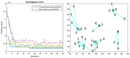
Figure 8.
Convergence curves and optimal distribution centers scheme for the IGA algorithm for six distribution centers.

Figure 9.
Convergence curves and optimal distribution centers scheme for the IGA algorithm for 10 distribution centers.
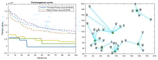
Figure 10.
Convergence curves and optimal distribution centers scheme for the CS algorithm for six distribution centers.
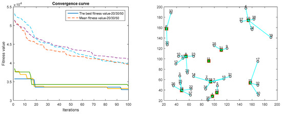
Figure 11.
Convergence curves and optimal distribution centers scheme for the CS algorithm for 10 distribution centers.

Figure 12.
Convergence curves and optimal distribution centers scheme for the CCS algorithm for six distribution centers.
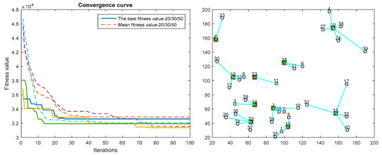
Figure 13.
Convergence curves and optimal distribution centers scheme for the CCS algorithm for 10 distribution centers.
Table 17.
Comparisons between DMQL-CS and other algorithms for six distribution centers.
Table 18.
Comparisons between DMQL-CS and other algorithms for 10 distribution centers.
For the third set of experiments, the CS algorithm was run 20, 30 and 50 times independently for the 40 city and six distribution center example. As shown in Figure 10, both the average convergence curve and the optimal convergence curve can converge at 80 iterations. The optimal distribution cost and average distribution cost obtained by the CS algorithm are 4.9629 × 10⁴ and 6.1392 × 10⁴, respectively. As shown in Figure 11, average convergence curve can converge at 100 iterations for 10 distribution centers. The optimal distribution cost and average distribution cost obtained by the CS algorithm are 3.2435 × 10⁴ and 3.9502 × 10⁴, which indicates that logistics distribution location strategy of CS algorithm is the worst in both the optimal convergence curve and the average convergence curve. Convergence curve of CCS algorithm can converge at 20 iterations in both the optimal convergence curve and the average convergence curve. CCS algorithm is much inferior to DMQL-CS algorithm in solving accuracy for 6 and 10 distribution centers. Although the IGA algorithm can converge, it has a lot of noise for the average convergence curve. The convergence effect of IGA is worse compared with CCS algorithm. The results of standard deviation indicate that DMQL-CS has a better robustness than the other algorithms. The optimal distribution centers and distribution addressing schemes are shown in Table 17 and Table 18. According to Table 17 and Table 18, the optimal distribution center points found by CS algorithm for 6 and 10 distribution centers are (3, 11, 22, 1, 15, 20) and (6, 8, 18, 11, 21, 28, 16, 1, 20, 15). The optimal distribution center points found by IGA algorithm for 6 and 10 distribution centers are (10, 22, 21, 2, 20, 17) and (30, 23, 14, 1, 2, 11, 25, 24, 15, 4). The optimal distribution center points found by CCS algorithm for 6 and 10 distribution centers are (23, 22, 21, 16, 15, 20) and (6, 10, 23, 14, 22, 25, 7, 16, 15, 20).
To further analyze the effectiveness of DMQL-CS algorithm, DMQL-CS was compared with four algorithms: CS [69], CCS [68], ICS [101], and IGA [64]. The comparison results with average fitness value (Mean), the best fitness value (Best), the worst fitness value (Worst), standard deviation (Std), and running time (Time) are shown in Table 19. It can be seen that the average distribution cost of DMQL-CS at six distribution centers is 4.8060 × 10⁴ which is 13,332 lower than CS, and the average distribution cost in 10 distribution centers is 3.0157 × 10⁴, which is 9345 lower than CS. Therefore, DMQL-CS is obviously superior to CS algorithm. Although ICS can provide far better final results for most of the cases, it takes more execution time because of the use of more expensive exploration operation during the initial phases. For 6 and 10 distribution centers, there is not much difference between ICS and DMQL-CS for average distribution cost, but the optimal distribution cost of DMQL-CS is significantly higher than that of ICS algorithm. Meanwhile, from the standard deviation and running time data, it can be known that DMQL-CS has better robustness. The IGA algorithm achieved the worst performance compared with other comparison algorithms, except for the CS algorithm. For the six distribution centers, the average value obtained by IGA algorithm is 5.3008 × 10⁴, which is 4948 more than DMQL-CS. The average value obtained by IGA algorithm is 3.6460 × 10⁴, which is 6330 more than DMQL-CS for 10 distribution centers. CCS algorithm obtains the third best performance for 6 and 10 distribution center, respectively. In summary, the results of DMQL-CS are better than the comparison algorithms in terms of optimal value, worst value, average value, or running time. The reason may be that the Q-learning step size strategy improves the precision of the algorithm. The crossover and mutation operator accelerate the convergence speed of the algorithm. Overall, the selection method of logistics distribution center based on cuckoo search algorithm with Q-Learning and genetic operation has better optimal value compared with the five other algorithms for both 6 and 10 distribution centers, which indicates that the selection strategy based on DMQL-CS has higher solution accuracy and wider range of optimization. Meanwhile, it can be seen in Table 19 that the running time of DMQL-CS is significantly lower than the four other algorithms, and the number of iterations is significantly reduced. In general, DMQL-CS algorithm can select the address of logistics distribution center more quickly and accurately compared with the comparison algorithm. Finally, we can say that our proposed algorithm interestingly outperforms other competitive algorithms in terms of convergence rate and robustness.
Table 19.
Comparisons between DMQL-CS and other algorithms for 6 and 10 distribution centers in 40 cities.
6. Conclusions
In this study, we constructed a model of CS with Q-Learning and genetic operators, and then solved the address of logistics distribution center with DMQL-CS algorithm in which adopts Q-Learning scheme to learn the individual optimal step size strategy according to the effect of individual multi-steps. The most appropriate step size control strategy is chosen as a parameter for the current step size evolution of the cuckoo, which increases the adaptability of individual evolution. At the same time, to accelerate the convergence of the algorithm, genetic operators and hybrid operations are added to DMQL-CS algorithm. Crossover and mutation operations expand the search area of the population, and accelerate the convergence of the DMQL-CS algorithm.
To verify the performance of DMQL-CS, DMQL-CS was employed to solve fifteen benchmark test functions and CEC 2013 test suit. The results show that the proposed DMQL-CS algorithm clearly outperforms the standard CS algorithm. Comparing with some improved CS variants and DE variants, we found that DMQL-CS algorithm outperforms the other algorithms on a majority of benchmarks. In addition, the effectiveness of the proposed method was further verified by comparing with CS, ICS, CCS, and IGA for both 6 and 10 distribution centers.
In the future, we will focus our research work on the study of special cases to strengthen the algorithm in more complex conditions. We will determine how to generalize our work to handle combinatorial optimization problems and to extend DMQL-CS optimization algorithms to in the realistic engineering areas and feature selection for machine learning [102].
Author Contributions
Conceptualization, J.L.; methodology, H.L.; software, D.-d.X. and T.Z.; validation, T.T.; writing—original draft preparation, J.L. and H.L.; writing—review and editing, D.-d.X. and T.Z.; funding acquisition, J.L. and T.T.; All authors have read and agreed to the published version of the manuscript.
Funding
This work was supported by doctoral Foundation of Wuhan Technology and Business University (No. D2019010) and the National Natural Science Foundation of China (No. 61503220).
Acknowledgments
The authors would like to thank the anonymous reviewers and the editor for their careful reviews and constructive suggestions to help us improve the quality of this paper.
Conflicts of Interest
The authors declare that they have no conflicts of interest.
References
- Sang, H.-Y.; Pan, Q.-K.; Duan, P.-Y.; Li, J.-Q. An effective discrete invasive weed optimization algorithm for lot-streaming flowshop scheduling problems. J. Intell. Manuf. 2015, 29, 1337–1349. [Google Scholar] [CrossRef]
- Sang, H.-Y.; Pan, Q.-K.; Li, J.-Q.; Wang, P.; Han, Y.-Y.; Gao, K.-Z.; Duan, P. Effective invasive weed optimization algorithms for distributed assembly permutation flowshop problem with total flowtime criterion. Swarm Evol. Comput. 2019, 44, 64–73. [Google Scholar] [CrossRef]
- Li, M.; Xiao, D.; Zhang, Y.; Nan, H. Reversible data hiding in encrypted images using cross division and additive homomorphism. Signal Process. Image Commun. 2015, 39, 234–248. [Google Scholar] [CrossRef]
- Li, M.; Guo, Y.; Huang, J.; Li, Y. Cryptanalysis of a chaotic image encryption scheme based on permutation-diffusion structure. Signal Process. Image Commun. 2018, 62, 164–172. [Google Scholar] [CrossRef]
- Fan, H.; Li, M.; Liu, D.; Zhang, E. Cryptanalysis of a colour image encryption using chaotic APFM nonlinear adaptive filter. Signal Process. 2018, 143, 28–41. [Google Scholar] [CrossRef]
- Dong, W.; Shi, G.; Li, X.; Ma, Y.; Huang, F. Compressive sensing via nonlocal low-rank regularization. IEEE Trans. Image Process. 2014, 23, 3618–3632. [Google Scholar] [CrossRef]
- Zhang, Y.; Gong, D.; Hu, Y.; Zhang, W. Feature selection algorithm based on bare bones particle swarm optimization. Neurocomputin 2015, 148, 150–157. [Google Scholar] [CrossRef]
- Zhang, Y.; Song, X.-F.; Gong, D.-W. A return-cost-based binary firefly algorithm for feature selection. Inf. Sci. 2017, 418, 561–574. [Google Scholar] [CrossRef]
- Mao, W.; He, J.; Tang, J.; Li, Y. Predicting remaining useful life of rolling bearings based on deep feature representation and long short-term memory neural network. Adv. Mech. Eng. 2018, 10, 1687814018817184. [Google Scholar] [CrossRef]
- Jian, M.; Lam, K.-M.; Dong, J. Facial-feature detection and localization based on a hierarchical scheme. Inf. Sci. 2014, 262, 1–14. [Google Scholar] [CrossRef]
- Wang, G.-G.; Chu, H.E.; Mirjalili, S. Three-dimensional path planning for UCAV using an improved bat algorithm. Aerosp. Sci. Technol. 2016, 49, 231–238. [Google Scholar] [CrossRef]
- Wang, G.; Guo, L.; Duan, H.; Liu, L.; Wang, H.; Shao, M. Path planning for uninhabited combat aerial vehicle using hybrid meta-heuristic DE/BBO algorithm. Adv. Sci. Eng. Med. 2012, 4, 550–564. [Google Scholar] [CrossRef]
- Zhang, Y.; Gong, D.-w.; Gao, X.-z.; Tian, T.; Sun, X.-y. Binary differential evolution with self-learning for multi-objective feature selection. Inf. Sci. 2020, 507, 67–85. [Google Scholar] [CrossRef]
- Wang, G.-G.; Cai, X.; Cui, Z.; Min, G.; Chen, J. High performance computing for cyber physical social systems by using evolutionary multi-objective optimization algorithm. IEEE Trans. Emerg. Top. Comput. 2017. [Google Scholar] [CrossRef]
- Cui, Z.; Sun, B.; Wang, G.-G.; Xue, Y.; Chen, J. A novel oriented cuckoo search algorithm to improve DV-Hop performance for cyber-physical systems. J. Parallel Distrib. Comput. 2017, 103, 42–52. [Google Scholar] [CrossRef]
- Jian, M.; Lam, K.-M.; Dong, J. Illumination-insensitive texture discrimination based on illumination compensation and enhancement. Inf. Sci. 2014, 269, 60–72. [Google Scholar] [CrossRef]
- Jian, M.; Lam, K.M.; Dong, J.; Shen, L. Visual-patch-attention-aware saliency detection. IEEE Trans. Cybern. 2015, 45, 1575–1586. [Google Scholar] [CrossRef]
- Wang, G.-G.; Lu, M.; Dong, Y.-Q.; Zhao, X.-J. Self-adaptive extreme learning machine. Neural Comput. Appl. 2016, 27, 291–303. [Google Scholar] [CrossRef]
- Mao, W.; Zheng, Y.; Mu, X.; Zhao, J. Uncertainty evaluation and model selection of extreme learning machine based on Riemannian metric. Neural Comput. Appl. 2013, 24, 1613–1625. [Google Scholar] [CrossRef]
- Liu, G.; Zou, J. Level set evolution with sparsity constraint for object extraction. IET Image Process. 2018, 12, 1413–1422. [Google Scholar] [CrossRef]
- Rizk-Allah, R.M.; El-Sehiemy, R.A.; Deb, S.; Wang, G.-G. A novel fruit fly framework for multi-objective shape design of tubular linear synchronous motor. J. Supercomput. 2017, 73, 1235–1256. [Google Scholar] [CrossRef]
- Yi, J.-H.; Xing, L.-N.; Wang, G.-G.; Dong, J.; Vasilakos, A.V.; Alavi, A.H.; Wang, L. Behavior of crossover operators in NSGA-III for large-scale optimization problems. Inf. Sci. 2020, 509, 470–487. [Google Scholar] [CrossRef]
- Yi, J.-H.; Deb, S.; Dong, J.; Alavi, A.H.; Wang, G.-G. An improved NSGA-III Algorithm with adaptive mutation operator for big data optimization problems. Future Gener. Comput. Syst. 2018, 88, 571–585. [Google Scholar] [CrossRef]
- Sun, J.; Miao, Z.; Gong, D.; Zeng, X.-J.; Li, J.; Wang, G.-G. Interval multi-objective optimization with memetic algorithms. IEEE Trans. Cybern. 2019. [Google Scholar] [CrossRef] [PubMed]
- Feng, Y.; Wang, G.-G. Binary moth search algorithm for discounted {0-1} knapsack problem. IEEE Access 2018, 6, 10708–10719. [Google Scholar] [CrossRef]
- Feng, Y.; Wang, G.-G.; Wang, L. Solving randomized time-varying knapsack problems by a novel global firefly algorithm. Eng. Comput. 2018, 34, 621–635. [Google Scholar] [CrossRef]
- Abdel-Basset, M.; Zhou, Y. An elite opposition-flower pollination algorithm for a 0-1 knapsack problem. Int. J. Bio-Inspired Comput. 2018, 11, 46–53. [Google Scholar] [CrossRef]
- Yi, J.-H.; Wang, J.; Wang, G.-G. Improved probabilistic neural networks with self-adaptive strategies for transformer fault diagnosis problem. Adv. Mech. Eng. 2016, 8, 1–13. [Google Scholar] [CrossRef]
- Mao, W.; He, J.; Li, Y.; Yan, Y. Bearing fault diagnosis with auto-encoder extreme learning machine: A comparative study. Proc. Inst. Mech. Eng. Part C J. Mech. Eng. Sci. 2016, 231, 1560–1578. [Google Scholar] [CrossRef]
- Mao, W.; Feng, W.; Liang, X. A novel deep output kernel learning method for bearing fault structural diagnosis. Mech. Syst. Signal Process. 2019, 117, 293–318. [Google Scholar] [CrossRef]
- Duan, H.; Zhao, W.; Wang, G.; Feng, X. Test-sheet composition using analytic hierarchy process and hybrid metaheuristic algorithm TS/BBO. Math. Probl. Eng. 2012, 2012, 1–22. [Google Scholar] [CrossRef]
- Wang, G.G.; Tan, Y. Improving metaheuristic algorithms with information feedback models. IEEE Trans. Cybern. 2019, 49, 542–555. [Google Scholar] [CrossRef] [PubMed]
- Rong, M.; Gong, D.; Zhang, Y.; Jin, Y.; Pedrycz, W. Multidirectional prediction approach for dynamic multiobjective optimization problems. IEEE Trans. Cybern. 2019, 49, 3362–3374. [Google Scholar] [CrossRef] [PubMed]
- Gong, D.; Sun, J.; Miao, Z. A Set-Based Genetic Algorithm for Interval Many-Objective Optimization Problems. IEEE Trans. Evol. Comput. 2018, 22, 47–60. [Google Scholar] [CrossRef]
- Gong, D.; Sun, J.; Ji, X. Evolutionary algorithms with preference polyhedron for interval multi-objective optimization problems. Inf. Sci. 2013, 233, 141–161. [Google Scholar] [CrossRef]
- Sergeyev, Y.D.; Kvasov, D.E.; Mukhametzhanov, M.S. On the efficiency of nature-inspired metaheuristics in expensive global optimization with limited budget. Sci. Rep. 2018, 8, 453. [Google Scholar] [CrossRef]
- Kvasov, D.E.; Mukhametzhanov, M.S. Metaheuristic vs. deterministic global optimization algorithms: The univariate case. Appl. Math. Comput. 2018, 318, 245–259. [Google Scholar] [CrossRef]
- Sergeyev, Y.D.; Kvasov, D.E.; Mukhametzhanov, M.S. Operational zones for comparing metaheuristic and deterministic one-dimensional global optimization algorithms. Math. Comput. Simul. 2017, 141, 96–109. [Google Scholar] [CrossRef]
- Yang, X.S.; Gandomi, A.H. Bat algorithm: A novel approach for global engineering optimization. Eng. Comput. 2012, 29, 464–483. [Google Scholar] [CrossRef]
- Simon, D. Biogeography-based optimization. IEEE Trans. Evol. Comput. 2008, 12, 702–713. [Google Scholar] [CrossRef]
- Dorigo, M.; Stutzle, T. Ant Colony Optimization; MIT Press: Cambridge, MA, USA, 2004. [Google Scholar]
- Wang, G.-G.; Deb, S.; Coelho, L.d.S. Earthworm optimization algorithm: A bio-inspired metaheuristic algorithm for global optimization problems. Int. J. Bio-Inspired Comput. 2018, 12, 1–22. [Google Scholar] [CrossRef]
- Wang, G.-G.; Deb, S.; Coelho, L.d.S. Elephant herding optimization. In Proceedings of the 2015 3rd International Symposium on Computational and Business Intelligence (ISCBI), Bali, Indonesia, 7–9 December 2015; pp. 1–5. [Google Scholar]
- Wang, G.-G.; Deb, S.; Gao, X.-Z.; Coelho, L.d.S. A new metaheuristic optimization algorithm motivated by elephant herding behavior. Int. J. Bio-Inspired Comput. 2016, 8, 394–409. [Google Scholar] [CrossRef]
- Wang, G.-G. Moth search algorithm: A bio-inspired metaheuristic algorithm for global optimization problems. Memetic Comput. 2018, 10, 151–164. [Google Scholar] [CrossRef]
- Yang, X.S. Firefly algorithm, stochastic test functions and design optimisation. Int. J. Bio-Inspired Comput. 2010, 2, 78–84. [Google Scholar] [CrossRef]
- Wang, H.; Yi, J.-H. An improved optimization method based on krill herd and artificial bee colony with information exchange. Memetic Comput. 2018, 10, 177–198. [Google Scholar] [CrossRef]
- Karaboga, D.; Basturk, B. A powerful and efficient algorithm for numerical function optimization: Artificial bee colony (ABC) algorithm. J. Glob. Optim. 2007, 39, 459–471. [Google Scholar] [CrossRef]
- Liu, F.; Sun, Y.; Wang, G.-G.; Wu, T. An artificial bee colony algorithm based on dynamic penalty and chaos search for constrained optimization problems. Arab. J. Sci. Eng. 2018, 43, 7189–7208. [Google Scholar] [CrossRef]
- Geem, Z.W.; Kim, J.H.; Loganathan, G.V. A new heuristic optimization algorithm: Harmony search. Simulation 2001, 76, 60–68. [Google Scholar] [CrossRef]
- Wang, G.-G.; Gandomi, A.H.; Zhao, X.; Chu, H.E. Hybridizing harmony search algorithm with cuckoo search for global numerical optimization. Soft Comput. 2016, 20, 273–285. [Google Scholar] [CrossRef]
- Wang, G.-G.; Deb, S.; Cui, Z. Monarch butterfly optimization. Neural Comput. Appl. 2019, 31, 1995–2014. [Google Scholar] [CrossRef]
- Wang, G.-G.; Deb, S.; Zhao, X.; Cui, Z. A new monarch butterfly optimization with an improved crossover operator. Oper. Res. Int. J. 2018, 18, 731–755. [Google Scholar] [CrossRef]
- Kennedy, J.; Eberhart, R. Particle swarm optimization. In Proceedings of the IEEE International Conference on Neural Networks, Perth, Australia, 27 November–1 December 1995; pp. 1942–1948. [Google Scholar]
- Sun, Y.; Jiao, L.; Deng, X.; Wang, R. Dynamic network structured immune particle swarm optimisation with small-world topology. Int. J. Bio-Inspired Comput. 2017, 9, 93–105. [Google Scholar] [CrossRef]
- Gandomi, A.H.; Alavi, A.H. Multi-stage genetic programming: A new strategy to nonlinear system modeling. Inf. Sci. 2011, 181, 5227–5239. [Google Scholar] [CrossRef]
- Gandomi, A.H.; Alavi, A.H. Krill herd: A new bio-inspired optimization algorithm. Commun. Nonlinear Sci. Numer. Simul. 2012, 17, 4831–4845. [Google Scholar] [CrossRef]
- Wang, G.-G.; Gandomi, A.H.; Alavi, A.H. An effective krill herd algorithm with migration operator in biogeography-based optimization. Appl. Math. Model. 2014, 38, 2454–2462. [Google Scholar] [CrossRef]
- Wang, G.-G.; Gandomi, A.H.; Alavi, A.H.; Deb, S. A multi-stage krill herd algorithm for global numerical optimization. Int. J. Artif. Intell. Tool 2016, 25, 1550030. [Google Scholar] [CrossRef]
- Wang, G.-G.; Gandomi, A.H.; Alavi, A.H.; Gong, D. A comprehensive review of krill herd algorithm: Variants, hybrids and applications. Artif. Intell. Rev. 2019, 51, 119–148. [Google Scholar] [CrossRef]
- Wang, G.-G.; Guo, L.; Gandomi, A.H.; Hao, G.-S.; Wang, H. Chaotic krill herd algorithm. Inf. Sci. 2014, 274, 17–34. [Google Scholar] [CrossRef]
- Wang, G.-G.; Deb, S.; Gandomi, A.H.; Alavi, A.H. Opposition-based krill herd algorithm with Cauchy mutation and position clamping. Neurocomputing 2016, 177, 147–157. [Google Scholar] [CrossRef]
- Wang, G.-G.; Gandomi, A.H.; Alavi, A.H. Stud krill herd algorithm. Neurocomputing 2014, 128, 363–370. [Google Scholar] [CrossRef]
- Wang, X.; Zhang, X.J.; Cao, X.; Zhang, J.; Fen, L. An improved genetic algorithm based on immune principle. Minimicro Syst. 1999, 20, 120. [Google Scholar]
- Li, J.; Li, Y.-x.; Tian, S.-s.; Zou, J. Dynamic cuckoo search algorithm based on Taguchi opposition-based search. Int. J. Bio-Inspired Comput. 2019, 13, 59–69. [Google Scholar] [CrossRef]
- Yang, X.S.; Deb, S. Engineering optimisation by cuckoo search. Int. J. Math. Model. Numer. Optim. 2010, 1, 330–343. [Google Scholar] [CrossRef]
- Gandomi, A.H.; Yang, X.-S.; Alavi, A.H. Cuckoo search algorithm: A metaheuristic approach to solve structural optimization problems. Eng. Comput. 2013, 29, 17–35. [Google Scholar] [CrossRef]
- Wang, G.-G.; Deb, S.; Gandomi, A.H.; Zhang, Z.; Alavi, A.H. Chaotic cuckoo search. Soft Comput. 2016, 20, 3349–3362. [Google Scholar] [CrossRef]
- Yang, X.-S.; Deb, S. Cuckoo search via Lévy flights. In Proceedings of the 2009 World Congress on Nature & Biologically Inspired Computing (NaBIC), Coimbatore, India, 9–11 December 2009; pp. 210–214. [Google Scholar]
- Mlakar, U.; Fister, I.; Fister, I. Hybrid self-adaptive cuckoo search for global optimization. Swarm Evol. Comput. 2016, 29, 47–72. [Google Scholar] [CrossRef]
- Li, X.; Wang, J.; Yin, M. Enhancing the performance of cuckoo search algorithm using orthogonal learning method. Neural Comput. Appl. 2013, 24, 1233–1247. [Google Scholar] [CrossRef]
- Ouaarab, A.; Ahiod, B.; Yang, X.-S. Discrete cuckoo search algorithm for the travelling salesman problem. Neural Comput. Appl. 2013, 24, 1659–1669. [Google Scholar] [CrossRef]
- Wang, Y.-H.; Li, T.-H.S.; Lin, C.-J. Backward Q-learning: The combination of Sarsa algorithm and Q-learning. Eng. Appl. Artif. Intell. 2013, 26, 2184–2193. [Google Scholar] [CrossRef]
- Alexandridis, A.; Chondrodima, E.; Sarimveis, H. Cooperative learning for radial basis function networks using particle swarm optimization. Appl. Soft Comput. 2016, 49, 485–497. [Google Scholar] [CrossRef]
- Rakhshani, H.; Rahati, A. Snap-drift cuckoo search: A novel cuckoo search optimization algorithm. Appl. Soft Comput. 2017, 52, 771–794. [Google Scholar] [CrossRef]
- Samma, H.; Lim, C.P.; Saleh, J.M. A new reinforcement learning-based memetic particle swarm optimizer. Appl. Soft Comput. 2016, 43, 276–297. [Google Scholar] [CrossRef]
- Abed-alguni, B.H. Action-selection method for reinforcement learning based on cuckoo search algorithm. Arab. J. Sci. Eng. 2017, 43, 6771–6785. [Google Scholar] [CrossRef]
- Ma, H.-S.; Li, S.-X.; Li, S.-F.; Lv, Z.-N.; Wang, J.-S. An improved dynamic self-adaption cuckoo search algorithm based on collaboration between subpopulations. Neural Comput. Appl. 2018, 31, 1375–1389. [Google Scholar] [CrossRef]
- Li, X.; Yin, M. Modified cuckoo search algorithm with self adaptive parameter method. Inf. Sci. 2015, 298, 80–97. [Google Scholar] [CrossRef]
- Yang, B.; Miao, J.; Fan, Z.; Long, J.; Liu, X. Modified cuckoo search algorithm for the optimal placement of actuators problem. Appl. Soft Comput. 2018, 67, 48–60. [Google Scholar] [CrossRef]
- Li, J.; Li, Y.-X.; Tian, S.-S.; Xia, J.-L. An improved cuckoo search algorithm with self-adaptive knowledge learning. Neural Comput. Appl. 2019. [Google Scholar] [CrossRef]
- Cheng, J.; Wang, L.; Xiong, Y. Ensemble of cuckoo search variants. Comput. Ind. Eng. 2019, 135, 299–313. [Google Scholar] [CrossRef]
- Long, W.; Cai, S.; Jiao, J.; Xu, M.; Wu, T. A new hybrid algorithm based on grey wolf optimizer and cuckoo search for parameter extraction of solar photovoltaic models. Energy Convers. Manag. 2020, 203, 112243. [Google Scholar] [CrossRef]
- Zhang, Z.; Ding, S.; Jia, W. A hybrid optimization algorithm based on cuckoo search and differential evolution for solving constrained engineering problems. Eng. Appl. Artif. Intell. 2019, 85, 254–268. [Google Scholar] [CrossRef]
- Zhang, X.; Li, X.-T.; Yin, M.-H. Hybrid cuckoo search algorithm with covariance matrix adaption evolution strategy for global optimisation problem. Int. J. Bio-Inspired Comput. 2019, 13, 102–110. [Google Scholar] [CrossRef]
- Tang, H.; Xue, F. Cuckoo search algorithm with different distribution strategy. Int. J. Bio-Inspired Comput. 2019, 13, 234–241. [Google Scholar] [CrossRef]
- Ong, P.; Zainuddin, Z. Optimizing wavelet neural networks using modified cuckoo search for multi-step ahead chaotic time series prediction. Appl. Soft Comput. 2019, 80, 374–386. [Google Scholar] [CrossRef]
- Kamoona, A.M.; Patra, J.C. A novel enhanced cuckoo search algorithm for contrast enhancement of gray scale images. Appl. Soft Comput. 2019, 85, 105749. [Google Scholar] [CrossRef]
- Naidu, M.N.; Boindala, P.S.; Vasan, A.; Varma, M.R. Optimization of Water Distribution Networks Using Cuckoo Search Algorithm. In Advanced Engineering Optimization Through Intelligent Techniques; Springer: Singapore, 2020. [Google Scholar]
- Ibrahim, A.M.; Tawhid, M.A. A hybridization of cuckoo search and particle swarm optimization for solving nonlinear systems. Evol. Intell. 2019, 12, 541–561. [Google Scholar] [CrossRef]
- Osaba, E.; del Ser, J.; Camacho, D.; Bilbao, M.N.; Yang, X.-S. Community detection in networks using bio-inspired optimization: Latest developments, new results and perspectives with a selection of recent meta-heuristics. Appl. Soft Comput. 2020, 87, 106010. [Google Scholar] [CrossRef]
- Rath, A.; Samantaray, S.; Swain, P.C. Optimization of the Cropping Pattern Using Cuckoo Search Technique. In Smart Techniques for a Smarter Planet; Springer: Cham, Switzerland, 2019; p. 19. [Google Scholar]
- Abdel-Basset, M.; Wang, G.-G.; Sangaiah, A.K.; Rushdy, E. Krill herd algorithm based on cuckoo search for solving engineering optimization problems. Multimed. Tools Appl. 2017, 78, 3861–3884. [Google Scholar] [CrossRef]
- Cao, Z.; Lin, C.; Zhou, M.; Huang, R. Scheduling semiconductor testing facility by using cuckoo search algorithm with reinforcement learning and surrogate modeling. IEEE Trans. Autom. Sci. Eng. 2019, 16, 825–837. [Google Scholar] [CrossRef]
- Hu, H.; Li, X.; Zhang, Y.; Shang, C.; Zhang, S. Multi-objective location-routing model for hazardous material logistics with traffic restriction constraint in inter-city roads. Comput. Ind. Eng. 2019, 128, 861–876. [Google Scholar] [CrossRef]
- Wang, F.; He, X.-s.; Wang, Y. The cuckoo search algorithm based on Gaussian disturbance. J. Xi’an Polytech. Univ. 2011, 25, 566–569. [Google Scholar]
- Wang, F.; Luo, L.; He, X.S.; Wang, Y. Hybrid optimization algorithm of PSO and Cuckoo Search. In Proceedings of the 2011 2nd International Conference on Artificial Intelligence, Management Science and Electronic Commerce (AIMSEC), Dengleng, China, 8–10 August 2011; IEEE: Piscataway, NJ, USA, 2011. [Google Scholar]
- Brest, J.; Greiner, S.; Boskovic, B.; Mernik, M.; Zumer, V. Self-Adapting Control Parameters in Differential Evolution: A Comparative Study on Numerical Benchmark Problems. IEEE Trans. Evol. Comput. 2006, 10, 646–657. [Google Scholar] [CrossRef]
- Qin, A.K.; Huang, V.L.; Suganthan, P.N. Differential Evolution Algorithm with Strategy Adaptation for Global Numerical Optimization. IEEE Trans. Evol. Comput. 2009, 13, 398–417. [Google Scholar] [CrossRef]
- Liang, J.J.; Qin, A.K.; Suganthan, P.N.; Baskar, S. Comprehensive learning particle swarm optimizer for global optimization of multimodal functions. IEEE Trans. Evol. Comput. 2006, 10, 281–295. [Google Scholar] [CrossRef]
- Zhao, S.A.; Qu, C.W. An Improved Cuckoo Algorithm for Solving the Problem of Logistics Distribution Center Location. Math. Pract. Theory 2017, 47, 206–213. [Google Scholar]
- del Ser, J.; Osaba, E.; Molina, D.; Yang, X.-S.; Salcedo-Sanz, S.; Camacho, D.; Das, S.; Suganthan, P.N.; Coello, C.A.C.; Herrera, F. Bio-inspired computation: Where we stand and what’s next. Swarm Evol. Comput. 2019, 48, 220–250. [Google Scholar] [CrossRef]


© 2020 by the authors. Licensee MDPI, Basel, Switzerland. This article is an open access article distributed under the terms and conditions of the Creative Commons Attribution (CC BY) license (http://creativecommons.org/licenses/by/4.0/).