Cavitation Model Calibration Using Machine Learning Assisted Workflow

Abstract

Conventional cavitation assessment methodology in industrial and scientific applications generally depends on cavitation models utilizing homogeneous mixture assumption. These models have been extensively assessed, modified and expanded to account for deficiencies of their predecessors. Unfortunately, none of the proposed models can be classified as the universal solution for all engineering applications, with usage mainly directed by experience or general availability of the models. In this study we propose a workflow through which the empirical constants governing the phase change of the Kunz mixture cavitation model can be calibrated for a given application or a series of problems, with machine learning as a tool for parameter estimation. The proposed approach was validated on a three-dimensional propeller test case with results in excellent agreement for the case in question. Results for thrust and torque were within 2% with cavity extents differing by up to 20%. This is a significant improvement when compared to previously proposed parameters. Despite the lack of generalization due to the limited nature of the dataset on which the model was trained, the proposed parameters entail acceptable results for similar cases as well. The overall methodology is applicable to other problems as well and should lead to more accurate cavitation predictions.

1. Introduction

Cavitation, along with induced noise and vibrations, present a principal problem in highly turbulent flows typical for, e.g., rotating machinery. Associated material erosion and noise pollution are commonly addressed with the design modifications ensuing from experimental and empirical knowledge, while the Computational Fluid Dynamics (CFD) approach is used as a secondary tool, mainly due to partially limited numerical models that simulate the inception and growth of cavities. Although progress is evident [1,2], CFD is yet to be deemed a viable self-sufficient option for cavitation-aware designs.

Difficulties stem from the methodology utilized for cavitation assessment. Commonly, homogeneous mixture models are employed to predict the cavitating flow. Since their introduction [3], homogeneous models have been extensively modified, with the modifications addressing certain challenges (e.g., sheet and super cavitation) [4,5]. Although most models have been deemed sufficient for industrial applications, they fundamentally rely on assumptions, with homogeneity and isothermality being the principal ones. Consequently, mixture models are utilized mostly based on previous personal experience, recommendations and results from the literature.

The prevailing mixture models employed for cavitation analysis nowadays are Kunz [4], Zwart [6] and Schnerr–Sauer [7]. The latter does not require empirical constants to be assessed, but rather the number of bubbles in a unit volume to be specified. Works by Gaggero et al. [8] and Lidtke et al. [9] concluded that the Sauer model is both sufficiently stable and accurate, although noticeable discrepancies were noted. In later works, Gaggero and Villa [10] attempted to calibrate the Sauer model for propeller analysis. Even though the calibration was effective for two dimensional case, when employed for three-dimensional propeller analysis, the model overpredicted sheet cavitation and struggled with a cavitation rope vortex. Recently, a study by Viitanen et al. [11] confirmed the observations noted in [8]; despite different models, cavitation rope prediction is heavily influenced by grid refinements which minimize dissipation and thus conserve the rope. Zwart and Kunz models, unlike Schnerr–Sauer, utilize empirical constants; hence, their accuracy and applicability heavily depend on the values employed for a case in question. This is certainly a detriment, as for proper use a good estimate of the parameters is required. However, they can outperform the Sauer model if properly calibrated. This is especially true for the Kunz model [12]. Furthermore, the Zwart model requires the vapor bubble radius to be estimated; hence, in order to simplify the workflow, the Kunz model was chosen as the primary focus of this study.

In their works, Medvitz et al. [13] and Lindau et al. [14] analyzed the Kunz model and its applicability for common turbomachinery problems. The assessment conducted in Medvitz et al. focused on a two-dimensional centrifugal pump with empirical constants governing the changes from liquid to vapor and vapor to liquid set at $C_{dest}=100$ and $C_{prod}=1000$. A study by Lindau et al. evaluated a three-dimensional marine propeller where $C_{dest}=100$ and $C_{prod}=0.2$. Overall, Kunz model was able to capture the sheet cavitation adequately, with discrepancies on the leading edge and at the cavitation vortex rope. Bensow et al. [15] similarly noted that the Kunz model struggles with the cavitation rope, whereas sheet cavitation is predicted fairly, although somewhat overpredicted. A skewed propeller was analyzed by Lu et al. [16] with parameters equal to those in [13]. It was noted that the sheet cavitation was adequately captured, whereas the cavitation rope was either underpredicted or simply not captured. General limitations are therefore similar to previous works, with denser grids proposed as a possible solution to proper rope capture. Studies by Morgut et al. [17] and Zhou et al. [18] attempted to calibrate the empirical constants of the Kunz model with partial success. Different optimization techniques were in both cases employed on a two-dimensional NACA66 hydrofoil model to extract optimal values. Results from both studies differed and have had limited success with other three-dimensional problems. Despite this, optimization techniques have been typically considered as the only viable option for parameter calibration.

The aforementioned studies mostly utilized standard Reynolds-averaged Navier–Stokes (RANS) models in conjunction with a given cavitation model. Wu et al. [19] in their study assessed the influences of the standard k-$ϵ$ turbulence model and a filter-based model variant proposed by Johansen [20] on cavitation inception and growth. The authors determined that for higher cavitation numbers models behave similarly, whereas for lower values, due to the reduced viscous damping in filter-based model, cavitation structures can differ significantly. Turbulent viscosity, or rather its overprediction, was similarly suggested by Coutier-Delgosha et al. [21,22] through the course of several studies as a principle cause of the disagreements between experiments and k-$ϵ$ based models. The authors primarily focused on the RNG k-$ϵ$ model and concluded that the standard implementation produces quasi-stationary results which fail to capture cavitation shedding and therefore deviate from experimental observations. A modified variant of the turbulence model was hence proposed. A subsequent study by Coutier-Delgosha et al. [23] suggested LES (Large Eddy Simulation) and DES (Detached Eddy Simulation) simulations as alternatives to filter-based models and RANS models in general. Similarly, Kunz et al. [24] found DES simulations to be a significant improvement over traditional RANS approach. A study by Bensow [25] comparatively evaluated RANS, DES and LES models when analyzing cavitation over a hydrofoil. Corrected RANS models were deemed as an improvement but still underperformed when compared to DES and LES. Shi et al. [26] and Ji et al. [27] evaluated a PANS (Partially Averaged Navier—Stokes)-derived k-$ϵ$ model and concluded that it is superior when compared to traditional approaches. Recently, Kadivar et al. [28,29] in a series of studies investigated the validity of the PANS method and the Schnerr and Sauer model for cavitation analysis around a hydrofoil. The approach was implemented in open-source toolkit OpenFOAM and has demonstrated great potential.

Inconsistency in proposed approaches and empirical values leads to ambiguity when utilizing cavitation models. Consequently, predictions are usually inadequate, results questionable and the overall applicability of CFD hindered. Hence, in this study we propose an efficient and effective approach to Kunz model parameter calibration that utilizes machine learning. Initially, a series of three-dimensional CFD simulations using the open-source solution OpenFOAM was conducted. Results, both qualitative and quantitative, were incorporated into a unified database. By employing the state-of-the-art random forest algorithm, values for $C_{dest}$ and $C_{prod}$ were predicted, and subsequently validated with RANS and ultimately DES simulations.

2. CFD Setup

2.1. Governing Equations

Numerical analyses conducted in this study are inherently unsteady and consider an incompressible fluid mixture. Vapor and liquid phases are viewed as a cohesive fluid and hence share both pressure and velocity fields. Equations governing the flow and phase change in homogeneous mixture models are continuity (1), momentum (2) and volume fraction transport Equation (3):

$$\frac{\partial {\rho }_m}{\partial t}+\nabla \left({\rho }_m\mathbf{u}\right)=0$$

(1)

$$\frac{\partial {\rho }_m\mathbf{u}}{\partial t}+\nabla \left({\rho }_m\mathbf{u}\mathbf{u}\right)=-\nabla P+\nabla \tau +S$$

(2)

$$\frac{\partial \gamma }{\partial t}+\nabla \left(\gamma \mathbf{u}\right)=\frac{\dot{m}}{{\rho }_l}$$

(3)

where ${\rho }_m$ represents mixture density, $\mathbf{u}$ velocity, P local pressure of the fluid, $\tau$ stress tensor, S source, $\gamma$ liquid volume fraction, $\dot{m}$ mass transfer rate due to cavitation and ${\rho }_l$ density of the liquid.

2.2. Cavitation Model

The Kunz transport model introduced in 2000 [4] is a prime example of a modified mixture cavitation model that fundamentally behaves like many others, but with unique definitions of source and sink terms. The model presented by Kunz utilizes empirical constants $C_{prod}$ and $C_{dest}$ that govern the transformations from vapor to liquid and liquid to vapor, respectively; see (4) and (5) [4]:

$${\dot{m}}^{+}=\frac{C_{prod}{\rho }_v{({\alpha }_l-{\alpha }_{ng})}^2(1-{\alpha }_l-{\alpha }_{ng})}{t_{\infty }}$$

(4)

$${\dot{m}}^{-}=\frac{C_{dest}{\rho }_v{\alpha }_{l}min[0,p-p_v]}{(1/2{\rho }_l{U}_{\infty }^2)t_{\infty }}$$

(5)

where ${\rho }_l$ and ${\rho }_v$ are liquid and vapor density, ${\alpha }_l$ and ${\alpha }_{ng}$ liquid phase and non-condensable gas volume fractions, p is the pressure, $p_v$ is the vapor pressure, $U_{\infty }$ is the free-stream velocity and $t_{\infty }$ is the mean flow time scale. In some literature, the constants are referred to as $C_c$ and $C_v$. Proposed values for both parameters were 100, with later introduced modifications specific for certain applications [4,5,13].

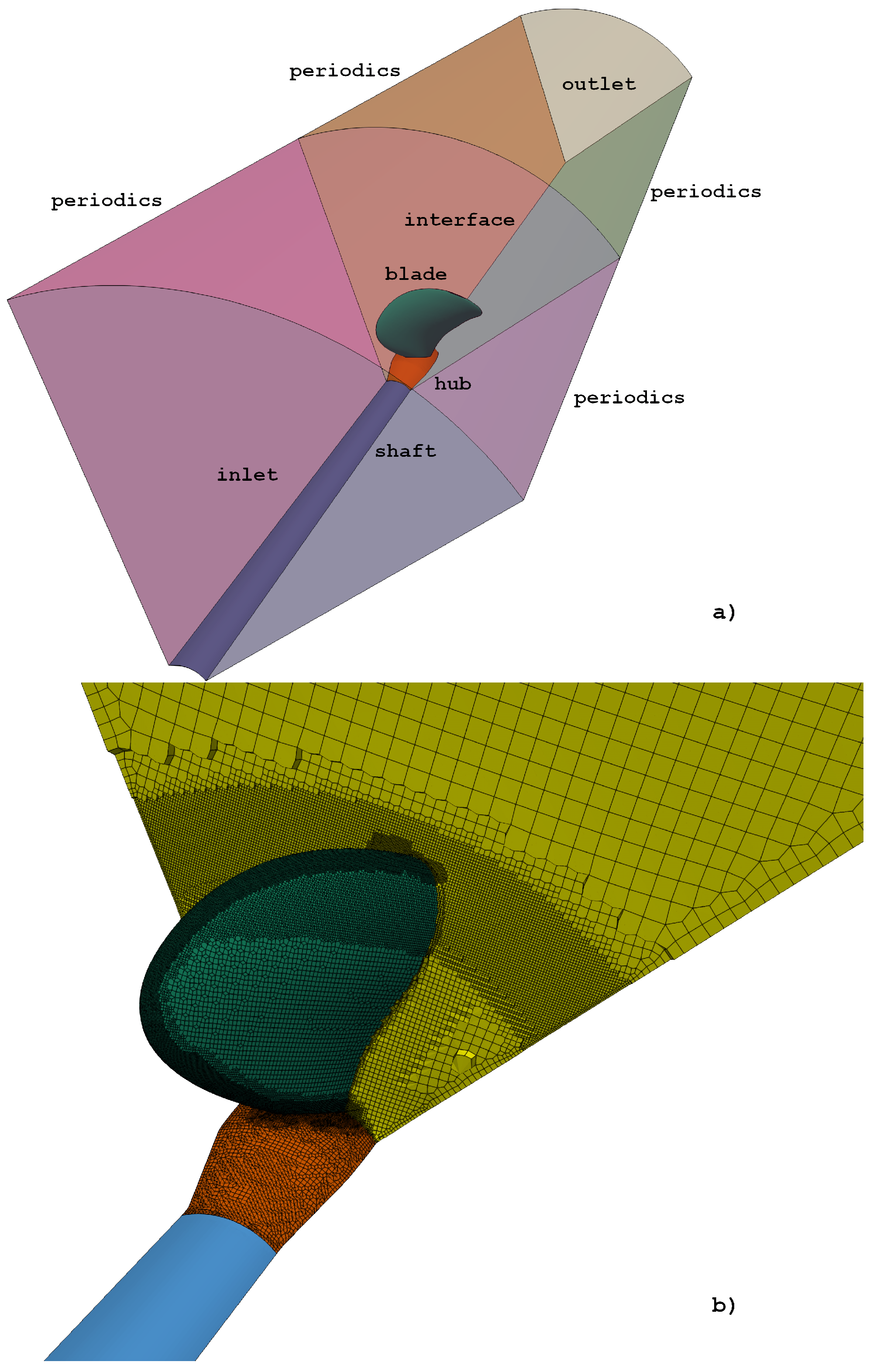
2.3. Geometry and Computational Domain

The geometric model used for calibration is a standard five-bladed VP1304 propeller. VP1304 is a conventional propeller for which both geometry and experimental data are provided by SVA Potsdam and is commonly referred to as the Potsdam propeller test case (PPTC) [30]. The geometry specifics of the propeller are given in

Table 1. VP1304 propeller geometry. [30].

Propeller diameter [m]	0.250
Pitch ratio at $r/R=0.7$	1.635
Chord length at $r/R=0.7$ [m]	0.104
Skew [${}^{\circ }$]	18.837
Hub ratio	0.300
Number of blades	5
Rotation	right

.

The computational domain enclosing the propeller has a circular cross-section where $D=0.6$ m. Overall length equals $L=2.6$ m. Positioning of the propeller is analogous to the experimental setup in the cavitation tunnel [30]. Simplification of the tunnel test section has been done in order to allow the execution of computationally affordable simulations on a periodic segment of the domain (one-fifth of the domain), thereby enabling successive evaluations of different test cases in order to provide data for the machine learning algorithm. An overview of the computational domain and key patches is shown in Figure 1.

2.4. Numerical Setup

Numerical analyses have been conducted in open-source CFD package OpenFOAM [31]. A transient, multiphase, incompressible solver utilizing the VOF (Volume of Fluid) approach for interface capturing, interPhaseChangeDyMFoam, was used to assess the cavitation. Kunz cavitation model was adopted to track the phase change [4]. The moving mesh paradigm we used simulated propeller motion. Primary fluid was water with kinematic viscosity of $\nu =9.337·{10}^{-7}$ m${}^2$/s. Specifics on case setup parameters can be found in the experimental documentation provided by SVA Potsdam [30]. The reference experimental setup is defined by advance ratio $J=1.0193$ and cavitation number ${\sigma }_n=2.024$. The Reynolds-averaged Navier–Stokes model [32], specifically the k-$\omega$ SST turbulence model, was used for all evaluations in the dataset and grid convergence study.

The Neumann boundary condition for velocity u has been prescribed at the outlet. The Dirichlet boundary condition through explicitly prescribed fixed values or fixed values which account for mesh movement (movingWallVelocity) has been used for other patches. For pressure, prgh, the Dirichlet boundary condition was set at the outlet, thereby enforcing a fixed value for the total pressure. Remaining patches had a Neumann boundary condition specified with included gradient correction on walls due to body forces (fixedFluxPressure). A water fraction alpha was fixed at the inlet with the Neumann boundary condition used for other patches. Values for turbulent viscosity ${\nu }_t$, turbulent kinetic energy k and the specific rate of dissipation $\omega$ at the inlet were estimated based on domain size and inflow velocity [32]; at walls, appropriate wall functions were used due to enforced $y^{+}$ value. Boundary conditions for all test cases are briefly summarized in

Table 2. An overview of the boundary conditions employed.

Field	Inlet	Outlet	Blades / Hub	Shaft
u	fixedValue	zeroGradient	movingWallVelocity	noSlip
prgh	zeroGradient	prghPressure	fixedFluxPressure	fixedFluxPressure
alpha	fixedValue	zeroGradient	zeroGradient	zeroGradient
${\nu }_t$	calculated	calculated	nutkWallFunction	nutkWallFunction
k	fixedValue	zeroGradient	kqRWallFunction	kqRWallFunction
$\omega$	fixedValue	zeroGradient	omegaWallFunction	omegaWallFunction

. Omitted boundaries included outer walls for which boundary conditions are equal to those used for stationary walls, apart from velocity, for which slip condition was set. Remaining patches were periodic faces and interfaces which used cyclicAMI and cyclicRepeatAMI boundary conditions respectively.

In the course of this study multiple test cases utilizing the same numerical grid and setup, albeit with altered Kunz mixture model parameters, have been evaluated. The described boundary conditions and overall setup were kept the same for all tests. Second-order schemes were used for alpha divergence terms with second-order upwind-biased schemes for the velocity. Upwind schemes were employed for turbulence fields with central differencing adopted for gradient terms. For the data collecting procedure a first-order implicit time scheme was used; DES simulations employed the second-order scheme. Convergence criteria for alpha have been fixed at ${10}^{-10}$ with ${10}^{-5}$ for other variables.

2.5. Grid Convergence

The numerical grid used in test cases was chosen from a set of pregenerated grids based on accuracy and computational requirements. Grids were generated with cfMesh, an open-source meshing solution for OpenFOAM. The largest cell size for the coarse grid equaled $\Delta =8·{10}^{-3}$ m. Refined grids utilized progressively smaller $\Delta$’s, with the finest grid utilizing $\Delta =5·{10}^{-3}$ m. Additional refinements around the blade edges, tip and region behind the propeller tip were included in order to better capture edge and rope cavitation. For all cases first cell height was kept at $\Delta y=2·{10}^{-4}$ m in order to maintain the dimensionless wall distance $30<y^{+}<60$. Consequently, appropriate wall functions had to be implemented to resolve the flow up to the wall.

Suitability of numerical grids has been evaluated on a single cavitation tunnel test case. interPhaseChangeDyMFoam solver and k-$\omega$ SST turbulence model were used to analyze the flow. Kunz model parameters for production and destruction were kept at their default values ($C_{prod}=C_{dest}=1$). The first-order implicit time scheme has been adopted. Second-order upwind-biased schemes for divergence and the central difference scheme for gradient terms were used. Pure upwind schemes were used for turbulence fields. Simulation time step was fixed and corresponds to $0.5^{\circ }$ of propeller rotation. The convergence criterion for all variables was set at ${10}^{-5}$. Results were analyzed after 1 s of simulation time.

Table 3. Grid details and grid convergence.

Mesh	Coarse	Medium	Fine
Grid Size	$1.1·{10}^6$	$1.93·{10}^6$	$3.59·{10}^6$
Max. Cell Size (m)	$8·{10}^{-3}$	$6.5·{10}^{-3}$	$5·{10}^{-3}$
Grid Refinement ratio	-	1.231	1.300
Relative Error (%)	-	0.983	0.758
GCI (%)	-	2.175	1.244

depicts grid specifics, including sizes and convergence by means of grid convergence index (GCI) [33]. Asymptotic behavior was achieved, as evidenced by convergence check $GC{I}_{2,3}/r^p·GC{I}_{1,2}\approx 0.992$.

Based on results presented in Table 3, a medium grid was deemed adequate for the proposed workflow. Due to the consistency of the results obtained in grid convergence study, values after 15 propeller revolutions were considered as sufficient for cavitation assessment. Hence, total simulation time was limited to ≈0.6 s with unchanged time stepping. Average Courant number was $Co\approx 0.32$, with a maximum of $Co\approx 21$.

3. Machine Learning Assisted Workflow

3.1. Challenges in Cavitation Analysis

Underlying uncertainty when utilizing different empirically obtained values is a common problem in cavitation analyses. Studies focusing on accurate cavitation predictions using mixture models commonly calibrate the parameters on a simple, two-dimensional case, to overcome this drawback. Optimized values are then employed to provide the cavitation prediction for a given problem. Although this approach seems intuitive, it is inherently flawed. The assumption that the two-dimensional and three-dimensional cases have any commonality is questionable, especially if we consider the empirical nature of the parameters. Furthermore, values are assessed on a case which is usually characterized by a different flow type, and hence the values obtained might be innate to said case, but not for the case for which those values are to be used. Generalization for other problems is also questionable, although it can be sometimes done, with varying success.

Here, we propose an alternative approach that has been made possible by the improvements in computational capabilities, which relies on advancements in the field of machine learning algorithms. The overall concept is rather simple; a series of CFD analyses on a specific case is conducted utilizing arbitrary empirical values for cavitation parameters. A machine learning algorithm is fed the data and consequently can be trained to provide acceptably accurate predictions for empirical parameters in question. The proposed methodology described in this work has been evaluated on a specific case, with the main benefits and drawbacks clearly presented. As is the case with all machine learning algorithms, the validity of the predictions mostly depends on the size of the dataset; hence, for extensive databases this approach can be leveraged to provide case-specific predictions.

3.2. ML Algorithm and Generalized Workflow

The concept of machine learning dates back to the second part of the twentieth century. Broadly, it can be described as a process in which a computer system is taught to predict or classify based on a pre-learned model extrapolated from an initial dataset, commonly referred to as a training set. The developed model is then validated on a known test set and can be consequently, with varying degrees of reliability and accuracy, employed to give predictions.

A fundamental prerequisite for any machine learning algorithm employed for the envisioned workflow is the ability to predict multiple (specifically two) outcome variables. Since outcome variables are continuous, the use of regression algorithms is necessary. The relationship between the outputs, however, is generally unknown, as the values in question are empirical. Consequently, simple regression models that can establish a correlation between the input data and a single continuous dependent variable can be employed consecutively to predict each of the required parameters independently. Therefore, a multiple regression model is a potential option as it can link multiple independent variables and a single dependent variable according to (6):

$$y=f(x_1,x_2,x_3\dots x_n)$$

(6)

Resulting model, however, will definitely not take into account the potential relationship between the input and the response variables as a whole; hence, a more pragmatic approach could provide better predictions. Multi-target regression is an obvious alternative, as it can establish a correlation between multiple independent and dependent variables (7):

$$y_1,y_2,y_3\dots y_n=f(x_1,x_2,x_3\dots x_n)$$

(7)

Random forests (RF) belong to a group of algorithms known as ensemble algorithms. They are built on top of decision trees and can be used to create strong prediction models by integrating weak models ensuing from each tree in the forest [34]. Although commonly used as classifiers, random forests are effective for regression problems as well. Compared to classification and regression trees (CART) [35], C4.5 [36] and conditional inference trees [37], which they are built upon, RFs are less deterministic, and hence exhibit less correlation, so can be used for better generalization [18]. Flexibility stems from randomness in feature (value) selection during the branching of the trees. This approach reduces bias and can minimize overfitting while also being adequate for smaller datasets. It is important to note, however, that the RF regression can not predict outside the scope of the training data, meaning that the continuous nature of the predictions is somewhat limited by the maxima and minima of the data RF was provided. This can be partially mitigated if a wider range of variables is utilized, which is the case in this study. Multivariate RF regression was therefore deemed adequate, chosen and implemented, to asses the empirical parameters for the Kunz cavitation model based on CFD-obtained predictions of propeller performance and cavity extents. An overview of the general workflow is given in Figure 2.

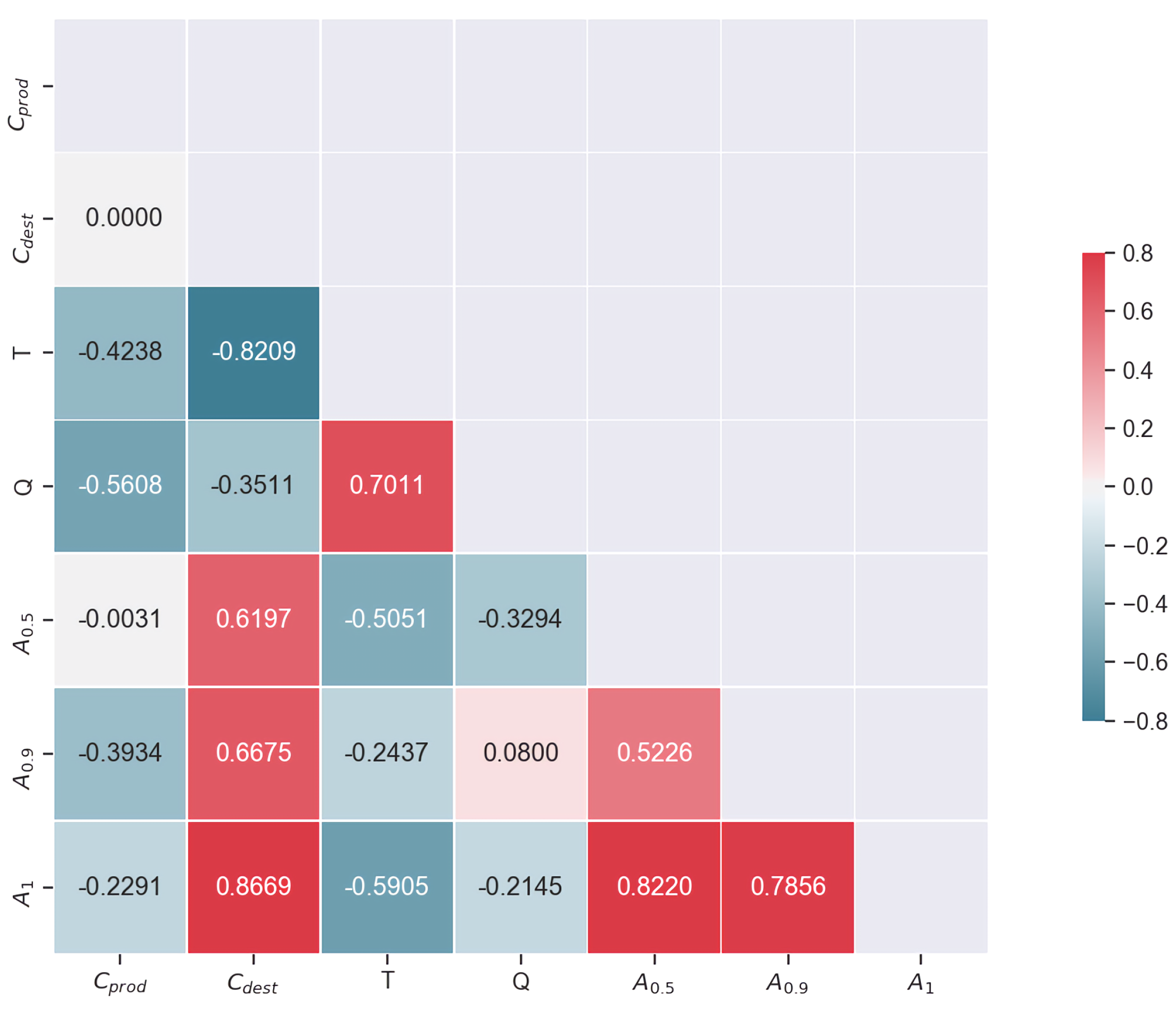
3.3. Data Analysis and Random Forest Regression

Data necessary to perform RF regression were obtained from a series of CFD simulations conducted according to the setup presented in Section 2.4. In total, 143 unique simulations have been conducted, each with a different set of empirical parameters $C_{prod}$ and $C_{dest}$. Values were defined on $0\le logX\le 4$ interval, where X denotes an empirical constant. For each simulation, propeller thrust T and torque Q have been logged. Furthermore, cavitation extents for 50% vapor volume fraction both on the blade and in the close proximity have been reported. Projected two-dimensional cavity extents at radial section $0\le r/R\le 0.5$ of the propeller are defined as surface $A_{0.5}$, at $0.5\le r/R\le 0.9$ as $A_{0.9}$ and for $0.9\le r/R\le 1$ as $A_1$. These zones roughly coincide with areas where hub, sheet and rope cavitation respectively occur, and were hence considered for machine learning. Simulations were carried out on an Intel E5-2690V3 based cluster with each case running on 40 threads. Average execution time of a simulation was 74 h.

Prior to training, the numerical results were subjected to min-max normalization. Correlations between the outcome variables ($C_{prod}$, $C_{dest}$) and previously described features (T, Q, $A_{0.5}$, $A_{0.9}$, $A_1$) are shown in Figure 3. It is evident that strong interdependence between $C_{dest}$ and cavity extents exists, with cavitation rope region $A_1$ being the most sensitive to parameter change. Based on these results we can conclude that $C_{dest}$ is the main driving force behind cavity expansion, which is consistent with the fact that it modifies the expression which governs the transformation from liquid to vapor (5).

A random forest regression model was implemented through python’s scikit-learn library [38]. For training, $80\%$ of the dataset was used, and $20\%$ was used for the final validation. Exclusion of the outliers was limited due to the rather small size of the dataset. Optimization of the hypperparameters for the RF algorithm revealed that the number of trees $n_{trees}=300$ (estimators) and a maximum depth of $n_{depth}=8$ produce the most consistent results. Effectiveness of the model was determined using typical criteria (8)–(10):

$$MAE=\frac{1}{N}\sum _{i=1}^N\left|{\widehat{y}}_{i,test}-y_{i,train}\right|$$

(8)

$$RMSE=\sqrt{\frac{1}{N}\sum _{i=1}^N{\left({\widehat{y}}_{i,test}-y_{i,train}\right)}^2}$$

(9)

$$MAPE=\frac{1}{N}\sum _{i=1}^N\left|\frac{{\widehat{y}}_{i,test}-y_{i,train}}{y_{i,train}}\right|·100\%$$

(10)

where $MAE$ corresponds to mean absolute error; $RMSE$ is root-mean-square error; $MAPE$ is mean absolute percentage error; $y_{train}$ and $y_{test}$ are actual and predicted values respectively. These metrics are commonly used to measure prediction accuracy of continuous variables [39]. An overview of the performance metrics for the employed algorithm is given in

Table 4. Summary of RF performance metrics.

Performance Metrics	MAE	RMSE	MAPE
Training Set (80%)	0.1558	0.1982	0.2852
Test Set (20%)	0.1583	0.2085	0.2966

.

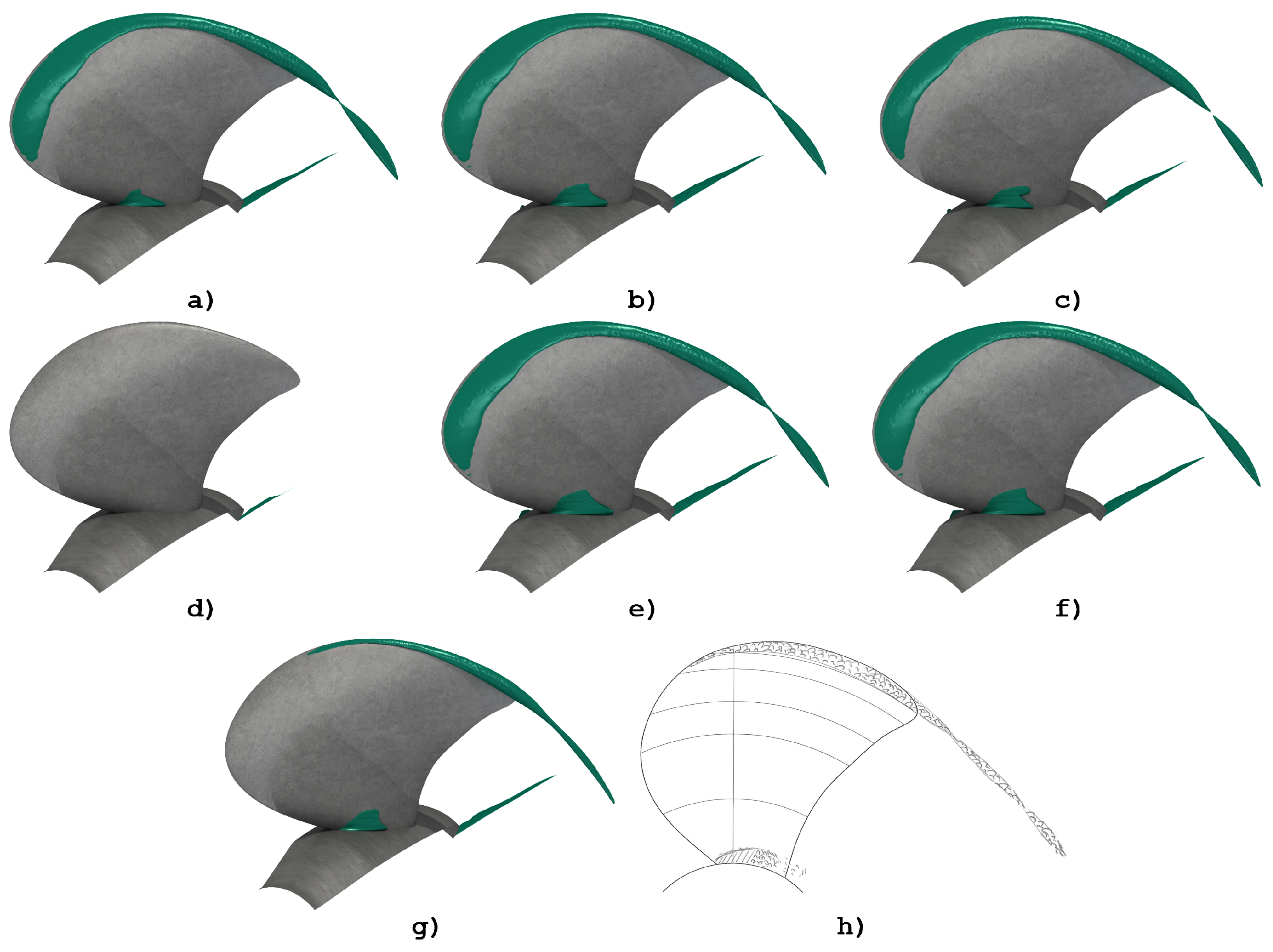
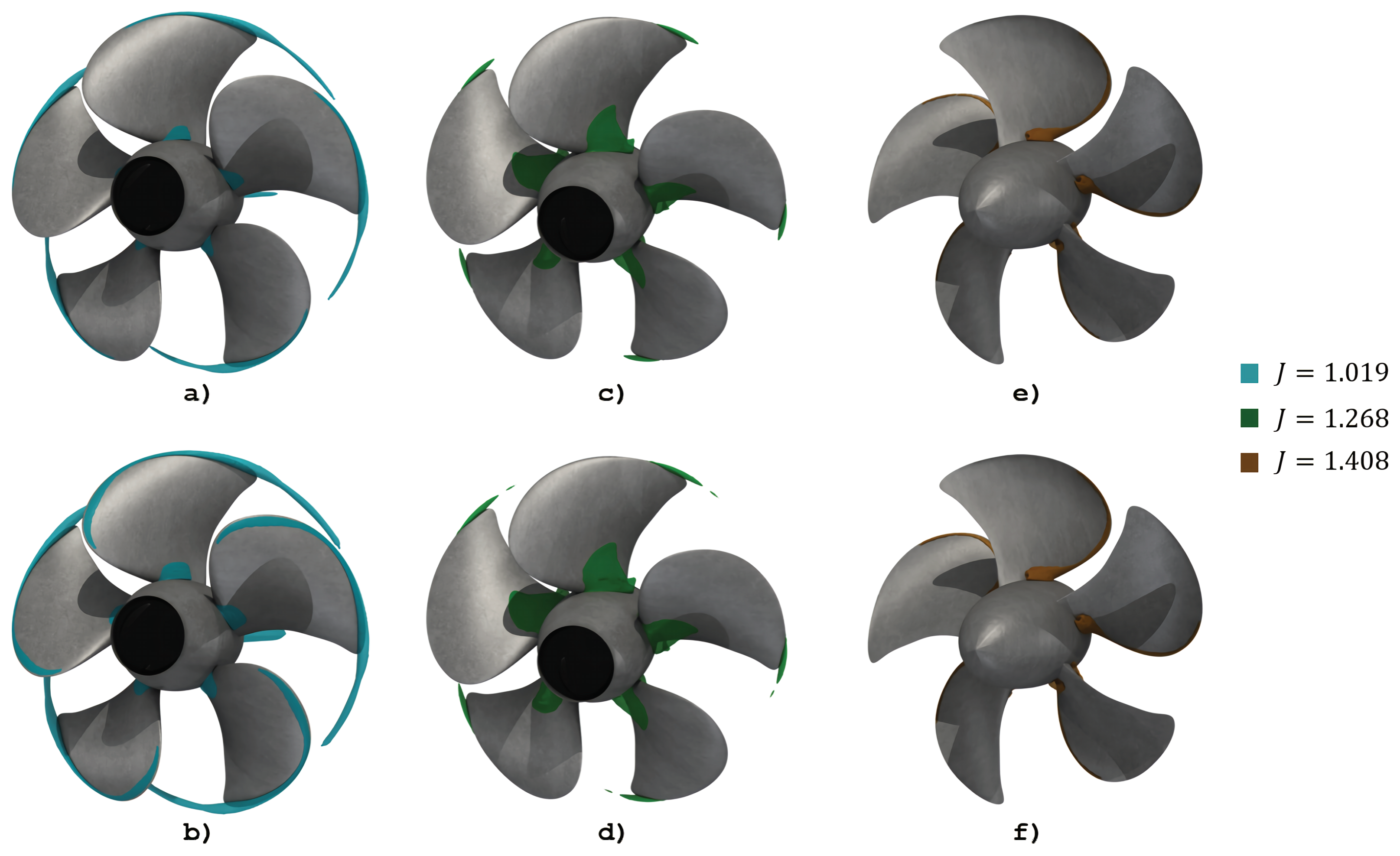
4. Predictions and Validity

The RF algorithm outlined in the previous section was employed to predict parameters suitable for cavitation analysis at $J=1.0193$ and ${\sigma }_n=2.024$. Values for thrust and torque were taken from the experimental report [30]. Cavitation extents near the hub ($A_{0.5}$), on the blade ($A_{0.9}$) and near the tip ($A_1$) were determined from the experimental observations [30]. The approximate experimental surface areas were ascertained by means of a simple image recognition algorithm written in python, with measurements of the blade subsequently correlated with the factual model size. Measured cavitation extents were scaled accordingly. It was assumed that noted extents are two-dimensional projections.

Outcomes of the random forest algorithm were $C_{prod}\approx 172$ and $C_{dest}\approx 5$. Broadly speaking, the predicted value for $C_{dest}$ was stable; hence, we do not expect a significant change in larger datasets either. Parameter $C_{prod}$ effectively limits the cavity collapse. Therefore, it is feasible to assume that higher values can be obtained if the intention is to further reduce cavitation extents. An overview of commonly employed empirical constants $C_{prod}$ and $C_{dest}$ in the literature, including predicted outcomes, is given in

Table 5. Common values for $C_{prod}$ and $C_{dest}$.

Reference	${\mathit{C}}_{\mathit{p}\mathit{r}\mathit{o}\mathit{d}}$	${\mathit{C}}_{\mathit{d}\mathit{e}\mathit{s}\mathit{t}}$
Bensow et al. [15]	20,000	1000
Morgut et al. [17]	455	4100
Kunz et al. [4]	100	100
Kunz et al. [5]	0.2	0.2
Vaz et al. [40]	10,000	500
Zhou et al. [41]	4328	3323
Predicted	172	5

.

Figure 4 illustrates disparity in cavity extents depending on $C_{prod}$ and $C_{dest}$. Included are experimental results, results obtained in this study and results for values presented in Table 5.

Quantitatively, the cavitation rope cavity is still overpredicted by ≈21%. The cavity near the hub is underpredicted by ≈20%. Sheet cavitation was non-existent for 50% vapor volume fraction, as was the case in the experiment. Thrust was overpredicted by 2% and torque underpredicted by 1%. Comparatively, these results are a significant improvement over the results obtained for the parameters proposed in literature [4,5,15,17,18,40], sometimes by several orders of magnitude. It is evident that random forests can extrapolate sufficiently accurate empirical parameters from limited datasests.

Parameter generalization has been assessed on an extended group of experimental cases where advance ratios are $J=1.268$ and $J=1.408$, utilizing k-$\omega$ SST DES turbulence model and the overall setup described in Section 2.4. Second-order time and divergence schemes were employed. Results are presented in Figure 5.

k-$\omega$ SST DES results are similar to RANS results both qualitatively and quantitatively. At $J=1.019$, thrust and torque are overpredicted by ≈2.7%. For $J=1.268$ and $J=1.408$ values are underpredicted by ≈0.3% and ≈3.52% respectively, both for thrust and for torque. Comparative results for RANS and DES models are given in

Table 6. Results for thrust (T) and torque (Q) obtained using RANS and DES models at different advance ratios J.

Case	${\mathit{T}}_{\mathit{e}\mathit{x}\mathit{p}.}$ (N)	${\mathit{T}}_{\mathit{R}\mathit{A}\mathit{N}\mathit{S}}$ (N)	${\mathit{T}}_{\mathit{D}\mathit{E}\mathit{S}}$ (N)	${\mathit{Q}}_{\mathit{e}\mathit{x}\mathit{p}.}$ (Nm)	${\mathit{Q}}_{\mathit{R}\mathit{A}\mathit{N}\mathit{S}}$ (Nm)	${\mathit{Q}}_{\mathit{D}\mathit{E}\mathit{S}}$ (Nm)
$J=1.019$	908.70	921.13	932.49	58.98	58.94	59.64
$J=1.268$	502.08	483.27	500.69	38.38	37.20	38.28
$J=1.408$	331.94	332.94	320.24	29.80	29.17	29.01

. Finer grid and lower time-stepping and full model simulations should reduce result discrepancy. Cavitation observations for 50% vapor volume fraction at $J=1.019$ are mostly in agreement to those obtained using RANS approach. Sheet cavitation for 20% vapor volume fraction was expected, as the calibration was done for 50% fraction. Observations at $J=1.268$ and $J=1.408$ show the best agreement with the experiment [30] at lower vapor volume fractions; extents for 10% fraction are in satisfactory agreement with errors similar to those for RANS cases (≈25%).

5. Discussion

Cavitation modeling using homogeneous mixture models introduces several challenges. The discrete border between the liquid and the vapor phases is absent; hence it is difficult to correlate experimental measurements and numerical results. In most cases, cavity extents are smeared due to numerical diffusivity. Constants governing the phase change in the, e.g., assessed Kunz model, are empirical; thus, they are usually case-specific. Due to all of this, certain assumptions have to be made in order to properly calibrate the model. The principal limitation is the vapor fraction reference which has for the purposes of this study been taken as 0.5.

Computational results utilized for the machine learning algorithm were gathered from a series of RANS simulations which were by definition averaged and grid and setup dependent. Potential issues arising from this can be mitigated by employing finer grids and complex turbulence models.

Random forest predictions depend on the accuracy of the results and the size of the dataset. Although RF’s are flexible, more data should lead to better, and depending on the type of the data, case-specific predictions. The image recognition algorithm utilized for prediction and validation introduces a point of failure when tracking cavity extents with additional assumptions of absolute accuracy of the noted experimental observations.

The results, specifically for the test case against which the model has been calibrated, are in excellent agreement with the experiment quantitatively and qualitatively, as evidenced by Figure 4. Unfortunately, previously mentioned deficiencies with regard to the missing interface between the phases and due to the limited test set led to observations which deviated more. Generalization of the parameters still needs to be assessed for similar problems.

The proposed methodology is a potential avenue through which machine learning assisted designs could eventually be generated with cavitation effects accounted for.

6. Conclusions

Calibrating a cavitation model is a complex, extensive and often case-specific task. This can be partially attributed to the empirical nature of the constants used in common homogeneous mixture models. Optimization methods are commonly employed in two-dimensional cases to predict the necessary parameters, which is in essence a flawed approach, as with this process a generalization from two to three dimensions is introduced. Although in certain conditions this might be fitting, it usually leads to the wrong results.

The methodology presented in this study employs a random forest regression algorithm on a dataset generated from a series of CFD simulations inherent to the case for which cavitation is to be assessed. Predicted empirical constants for the Kunz cavitation model, $C_{prod}\approx 172$ and $C_{dest}\approx 5$, induce cavities which are in excellent agreement with the experimental results, especially in contrast with other commonly used values. Quantitatively, errors are below 2%, while qualitatively cavity extents can differ up to 21%. These discrepancies are a significant improvement over existing results, notably for sheet cavitation. It is important to note, however, that the result is not universal, which is primarily due to the case-specific nature of the dataset itself. Further validation should incorporate different cases and advanced turbulence models with flow resolved up to the wall.

The concepts herein are applicable to different types of applications and inputs, including sectional pressure distributions. The workflow should be more efficient than a typical optimization, although larger databases will certainly lead to better predictions. Uncertainties introduced by the stochastic nature of the random forests can be mitigated by including additional data. Independently, the presented methodology, similarly to optimization, might be too case-specific; however, comprehensive standardized databases that include various cases and test sets could be leveraged to account for case-specific nature of predictions, which is a significant advantage.

References

1. Bertetta, D.; Brizzolara, S.; Gaggero, S.; Viviani, M.; Savio, L. CPP propeller cavitation and noise optimization at different pitches with panel code and validation by cavitation tunnel measurements. Ocean Eng. 2012, 53, 177–195. [Google Scholar] [CrossRef]
2. Gaggero, S.; Tani, G.; Villa, D.; Viviani, M.; Ausonio, P.; Travi, P.; Bizzarri, G.; Serra, F. Efficient and multi-objective cavitating propeller optimization: An application to a high-speed craft. Appl. Ocean Res. 2017, 64, 31–57. [Google Scholar] [CrossRef]
3. Kubota, A.; Kato, H.; Yamaguchi, H. A new modelling of cavitating flows: A numerical study of unsteady cavitation on a hydrofoil section. J. Fluid Mech. 1992, 240, 59–96. [Google Scholar] [CrossRef]
4. Kunz, R.F.; Boger, D.A.; Stinebring, D.R.; Chyczewski, T.S.; Lindau, J.W.; Gibeling, H.J.; Venkateswaran, S.; Govindan, T. A preconditioned Navier-Stokes method for two-phase flows with application to cavitation prediction. Comput. Fluids 2000, 29, 849–875. [Google Scholar] [CrossRef]
5. Kunz, R.F.; Boger, D.A.; Chyczewski, T.S.; Stinebring, D.; Gibeling, H.; Govindan, T. Multi-phase CFD analysis of natural and ventilated cavitation about submerged bodies. In Proceedings of the 3rd ASME-JSME Joint Fluids Engineering Conference, San Francisco, CA, USA, 18–23 July 1999. [Google Scholar]
6. Zwart, P.J.; Gerber, A.G.; Belamri, T. A two-phase flow model for predicting cavitation dynamics. In Proceedings of the Fifth International Conference on Multiphase Flow, Yokohama, Japan, 30 May–3 June 2004; Volume 152. [Google Scholar]
7. Schnerr, G.H.; Sauer, J. Physical and numerical modeling of unsteady cavitation dynamics. In Proceedings of the Fourth International Conference on Multiphase Flow, New Orleans, LA, USA, 27 May–1 June 2001; Volume 1. [Google Scholar]
8. Gaggero, S.; Tani, G.; Viviani, M.; Conti, F. A study on the numerical prediction of propellers cavitating tip vortex. Ocean Eng. 2014, 92, 137–161. [Google Scholar] [CrossRef]
9. Lidtke, A.K.; Humphrey, V.F.; Turnock, S.R. Feasibility study into a computational approach for marine propeller noise and cavitation modelling. Ocean Eng. 2016, 120, 152–159. [Google Scholar] [CrossRef] [Green Version]
10. Gaggero, S.; Villa, D. Steady cavitating propeller performance by using OpenFOAM, StarCCM+ and a boundary element method. Proc. Inst. Mech. Eng. Part M J. Eng. Marit. Environ. 2017, 231, 411–440. [Google Scholar] [CrossRef]
11. Viitanen, V.; Siikonen, T.; Sánchez-Caja, A. Cavitation on Model-and Full-Scale Marine Propellers: Steady And Transient Viscous Flow Simulations At Different Reynolds Numbers. J. Mar. Sci. Eng. 2020, 8, 141. [Google Scholar] [CrossRef] [Green Version]
12. Roohi, E.; Pendar, M.R.; Rahimi, A. Simulation of three-dimensional cavitation behind a disk using various turbulence and mass transfer models. Appl. Math. Model. 2016, 40, 542–564. [Google Scholar] [CrossRef]
13. Medvitz, R.B.; Kunz, R.F.; Boger, D.A.; Lindau, J.W.; Yocum, A.M.; Pauley, L.L. Performance analysis of cavitating flow in centrifugal pumps using multiphase CFD. J. Fluids Eng. 2002, 124, 377–383. [Google Scholar] [CrossRef]
14. Lindau, J.W.; Boger, D.A.; Medvitz, R.B.; Kunz, R.F. Propeller cavitation breakdown analysis. J. Fluids Eng. 2005, 127, 995. [Google Scholar] [CrossRef]
15. Bensow, R.E.; Bark, G. Implicit LES predictions of the cavitating flow on a propeller. J. Fluids Eng. 2010, 132, 041302. [Google Scholar] [CrossRef]
16. Lu, N.X.; Bensow, R.E.; Bark, G. Large eddy simulation of cavitation development on highly skewed propellers. J. Mar. Sci. Technol. 2014, 19, 197–214. [Google Scholar] [CrossRef]
17. Morgut, M.; Nobile, E.; Biluš, I. Comparison of mass transfer models for the numerical prediction of sheet cavitation around a hydrofoil. Int. J. Multiph. Flow 2011, 37, 620–626. [Google Scholar] [CrossRef]
18. Zhou, Z.H. Ensemble Methods: Foundations and Algorithms; CRC Press: Boca Raton, FL, USA, 2012. [Google Scholar]
19. Wu, J.; Utturkar, Y.; Shyy, W. Assessment of modeling strategies for cavitating flow around a hydrofoil. In Proceedings of the Fifth International Symposium on Cavitation, Osaka, Japan, 1–4 November 2003; pp. 1–5. [Google Scholar]
20. Johansen, S.T.; Wu, J.; Shyy, W. Filter-based unsteady RANS computations. Int. J. Heat Fluid Flow 2004, 25, 10–21. [Google Scholar] [CrossRef]
21. Coutier-Delgosha, O.; Reboud, J.; Delannoy, Y. Numerical simulation of the unsteady behaviour of cavitating flows. Int. J. Numer. Methods Fluids 2003, 42, 527–548. [Google Scholar]
22. Coutier-Delgosha, O.; Fortes-Patella, R.; Reboud, J.L. Evaluation of the turbulence model influence on the numerical simulations of unsteady cavitation. J. Fluids Eng. 2003, 125, 38–45. [Google Scholar] [CrossRef] [Green Version]
23. Coutier-Delgosha, O.; Deniset, F.; Astolfi, J.A.; Leroux, J.B. Numerical prediction of cavitating flow on a two-dimensional symmetrical hydrofoil and comparison to experiments. J. Fluids Eng. 2007, 129, 279–292. [Google Scholar] [CrossRef] [Green Version]
24. Kunz, R.F.; Lindau, J.W.; Kaday, T.A.; Peltier, L.J. Unsteady RANS and detached eddy simulations of cavitating flow over a hydrofoil. In Proceedings of the Fifth International Symposium on Cavitation, Osaka, Japan, 1–4 November 2003. [Google Scholar]
25. Bensow, R.E. Simulation of the unsteady cavitation on the Delft Twist11 foil using RANS, DES and LES. In Proceedings of the Second International Symposium on Marine Propulsors, Hamburg, German, 15–17 June 2011. [Google Scholar]
26. Shi, W.; Zhang, G.; Zhang, D. Evaluation of turbulence models for the numerical prediction of transient cavitation around a hydrofoil. IOP Conf. Ser. Mater. Sci. Eng. 2013, 52, 062013. [Google Scholar] [CrossRef] [Green Version]
27. Ji, B.; Luo, X.; Wu, Y.; Peng, X.; Duan, Y. Numerical analysis of unsteady cavitating turbulent flow and shedding horse-shoe vortex structure around a twisted hydrofoil. Int. J. Multiph. Flow 2013, 51, 33–43. [Google Scholar] [CrossRef] [Green Version]
28. Kadivar, E.; el Moctar, O.; Javadi, K. Investigation of the effect of cavitation passive control on the dynamics of unsteady cloud cavitation. Appl. Math. Model. 2018, 64, 333–356. [Google Scholar] [CrossRef]
29. Kadivar, E.; Timoshevskiy, M.V.; Pervunin, K.S.; el Moctar, O. Experimental and numerical study of the cavitation surge passive control around a semi-circular leading-edge flat plate. J. Mar. Sci. Technol. 2019, 25, 1–4. [Google Scholar] [CrossRef]
30. SVA Team. PPTC smp’11 Workshop. 2011. Available online: https://www.sva-potsdam.de/pptc-smp11-workshop/ (accessed on 18 July 2020).
31. The OpenFOAM Foundation. OpenFOAM User Guide. 2016. Available online: https://www.openfoam.org (accessed on 18 July 2020).
32. Ferziger, J.H.; Peric, M. Computational Methods for Fluid Dynamics; Springer Science & Business Media: Berlin/Heidelberg, Germany, 2012. [Google Scholar]
33. Roache, P.J. Verification and Validation in Computational Science and Engineering; Hermosa Publisher: Socorro, NM, USA, 1998; Volume 895. [Google Scholar]
34. Breiman, L. Random forests. Mach. Learn. 2001, 45, 5–32. [Google Scholar] [CrossRef] [Green Version]
35. Breiman, L.; Friedman, J.; Stone, C.J.; Olshen, R.A. Classification and Regression Trees; CRC Press: Boca Raton, FL, USA, 1984. [Google Scholar]
36. Quinlan, R. C4.5. In Programs for Machine Learning; Morgan Kaufmann Publishers: Burlington, MA, USA, 1993. [Google Scholar]
37. Hothorn, T.; Hornik, K.; Zeileis, A. Unbiased recursive partitioning: A conditional inference framework. J. Comput. Graph. Stat. 2006, 15, 651–674. [Google Scholar] [CrossRef] [Green Version]
38. Pedregosa, F.; Varoquaux, G.; Gramfort, A.; Michel, V.; Thirion, B.; Grisel, O.; Blondel, M.; Prettenhofer, P.; Weiss, R.; Dubourg, V.; et al. Scikit-learn: Machine learning in Python. J. Mach. Learn. Res. 2011, 12, 2825–2830. [Google Scholar]
39. Botchkarev, A. Performance metrics (error measures) in machine learning regression, forecasting and prognostics: Properties and typology. arXiv 2018, arXiv:1809.03006. [Google Scholar]
40. Vaz, G.; Hally, D.; Huuva, T.; Bulten, N.; Muller, P.; Becchi, P.; Herrer, J.L.; Whitworth, S.; Macé, R.; Korsström, A. Cavitating flow calculations for the E779A propeller in open water and behind conditions: Code comparison and solution validation. In Proceedings of the Fourth International Symposium on Marine Propulsors SMP, Austin, TX, USA, 31 May–4 June 2015; Volume 15, pp. 344–360. [Google Scholar]
41. Zhou, H.; Xiang, M.; Okolo, P.N.; Wu, Z.; Bennett, G.J.; Zhang, W. An efficient calibration approach for cavitation model constants based on OpenFOAM platform. J. Mar. Sci. Technol. 2019, 24, 1043–1056. [Google Scholar] [CrossRef]
Figure 1. Details of the numerical setup. (a) Computational domain with relevant patches and (b) cross-sectional detail of a coarse mesh.
Mathematics 08 02107 g001
Figure 2. Proposed workflow utilizing a random forest algorithm. Numerical simulations were used to create a dataset in which relevant performance parameters and cavitation observations were stored. An RF regression algorithm was employed to provide predictions for C p r o d and C d e s t . Results were validated against experimental observations and further confirmed with DES analysis.
Mathematics 08 02107 g002
Figure 3. Correlation matrix. Observations are consistent with the Kunz model’s definition.
Mathematics 08 02107 g003
Figure 4. Cavity extents for vapor volume fraction of 0.5 when utilizing various values of parameters C p r o d and C d e s t from the literature. (a) Bensow et al. [15], (b) Morgut et al. [17], (c) Kunz et al. [4], (d) Kunz et al. [5], (e) Vaz et al. [40], (f) Zhou et al. [41], (g) predicted values C p r o d = 172 , C d e s t = 5 and (h) experimental observations [30].
Mathematics 08 02107 g004
Figure 5. Cavitation patterns obtained using k- ω SST DES turbulence model. Results show good agreement with the experiment [30]. (a) Results for J = 1.019 , σ = 2.024 at 50% vapor volume fraction and (b) 20% vapor volume fraction; (c) J = 1.268 , σ = 1.424 at 20% vapor volume fraction and (d) 10% vapor volume fraction; (e) J = 1.408 , σ = 1.999 at 20% vapor volume fraction and (f) 10% vapor volume fraction.
Mathematics 08 02107 g005