Article

TOPSIS Decision on Approximate Pareto Fronts by Using Evolutionary Algorithms: Application to an Engineering Design Problem

by
Máximo Méndez
1,*,†,
Mariano Frutos
2,†,
Fabio Miguel
3,† and
Ricardo Aguasca-Colomo
1,†
1
Instituto Universitario SIANI, Universidad de Las Palmas de Gran Canaria (ULPGC), 35017 Las Palmas de G.C., Spain
2
Department of Engineering, Universidad Nacional del Sur and CONICET, Bahía Blanca 8000, Argentina
3
Universidad Nacional de Río Negro, Sede Alto Valle y Valle Medio, Villa Regina 8336, Argentina
*
Author to whom correspondence should be addressed.
These authors contributed equally to this work.
Mathematics 2020, 8(11), 2072; https://doi.org/10.3390/math8112072
Submission received: 20 October 2020 / Revised: 9 November 2020 / Accepted: 17 November 2020 / Published: 20 November 2020
(This article belongs to the Section Mathematics and Computer Science)

Abstract

:
A common technique used to solve multi-objective optimization problems consists of first generating the set of all Pareto-optimal solutions and then ranking and/or choosing the most interesting solution for a human decision maker (DM). Sometimes this technique is referred to as generate first–choose later. In this context, this paper proposes a two-stage methodology: a first stage using a multi-objective evolutionary algorithm (MOEA) to generate an approximate Pareto-optimal front of non-dominated solutions and a second stage, which uses the Technique for Order Preference by Similarity to an Ideal Solution (TOPSIS) devoted to rank the potential solutions to be proposed to the DM. The novelty of this paper lies in the fact that it is not necessary to know the ideal and nadir solutions of the problem in the TOPSIS method in order to determine the ranking of solutions. To show the utility of the proposed methodology, several original experiments and comparisons between different recognized MOEAs were carried out on a welded beam engineering design benchmark problem. The problem was solved with two and three objectives and it is characterized by a lack of knowledge about ideal and nadir values.

1. Introduction

When real Multi-objective Optimization Problems (MOPs) are tackled, two different working approaches can be identified in the literature. The first, known as Multiple Criteria Decision-Making (MCDM) [1,2,3,4,5,6,7,8,9,10,11,12,13], is essentially interested in decision-making, for example in helping a human Decision-Maker (DM) to choose between various alternatives or solutions in accordance with several conflicting criteria or objectives. The main representatives of this approach can be found in schools of economics, management and finance and the role and participation of the DM before and during the decision-making process are decisive. The second, Multi-Objective Optimization (MOO) [14,15,16,17,18,19], more to the taste of engineers and mathematicians, is related to highly complex optimization problems, where, rather than the decision, the major interest lies in using fast algorithms to find a non-dominated set of solutions or Pareto-soptimal Front (POF). In this approach, DM participation in the search process may not be necessary. MCDM and MOO are therefore two disciplines belonging to two different scientific communities, who solve similar problems and communicate with one another but have different competences.
The population-based Multi-Objective Evolutionary Algorithms (MOEA) [20,21,22,23,24,25,26,27,28,29,30,31], rather popular among the MOO scientific community, have shown a remarkable performance when solving hard optimization problems. These algorithms do not guarantee the determination of the exact POF, but the result is very close to the exact solution. Most MOEAs are categorized as a posteriori preference articulation, also referred to as Generate First–Choose Later (GFCL) [27,32]. The idea involves first generating multiple optimal Pareto solutions followed by choosing the most preferred one according to some criteria. The Non-Dominated Sorting Genetic Algorithm-II (NSGA-II) [33], the Multi-Objective Evolutionary Algorithm based on Decomposition (MOEA/D) [34] and the Global Weighting Achievement Scalarizing Function Genetic Algorithm (GWASF-GA) [35], to cite only three of the many relevant MOEAs, are recognized algorithms in the multi-objective literature that use this approach. NSGA-II is based on Pareto’s dominance as a criterion to converge to the POF and crowding-distance operator as increasing diversification in the population. MOEA/D uses a strategy of decomposing the MOP into several scalar sub-problems that are simultaneously solved by the evolution of a population of solutions. GWASF-GA incorporates the ideas of NSGA-II and MOEA/D and it classifies solutions on Pareto fronts but based on the achievement scalarizing function of Wierzbicki [36]. On the other hand, Branke [37] suggested that, if a DM has some idea about what solutions to the problem might be preferred, this knowledge should be exploited. In this line, Branke proposed the integration of this imprecise knowledge (partial user preferences) in a MOEA, with the purpose of focusing the search for solutions in that region of the POF that is most relevant for the DM. The final result of this approach is a small region of the POF which contains the most likely preferred solutions for DM and from which the DM will select a solution. This approach also assumes a GFCL methodology and some examples that include DM’s partial-preferences as a reference point are reported in [38,39,40,41,42,43,44]. The Non-g-Dominated Sorting Genetic Algorithm (g-NSGA-II in this work) modifies the dominance of Pareto in the original NSGA-II because of the g-dominance relation proposed in [41]. The Weighting Achievement Scalarizing Function Genetic Algorithm (WASF-GA) [43], similar to NSGA-II, devises the population of individuals into several fronts but based on the achievement scalarizing function of Wierzbicki [36] for each vector of weights in a sample of the weight vector space.
MOEAs have extensive applications in the engineering field [45] and, some of them, propose a two-stage methodology. The first stage, using some evolutionary method, is dedicated to building the best POF of solutions. The second stage engages some MCDM technique to select the most attractive one. This methodology has shown excellent potential in various optimization problems. In [46], a two-stage approach for solving multi-objective system reliability optimization problems is proposed. A POF is initially identified at the first stage by applying a MOEA. Quite often there are a large number of Pareto optimal solutions, and it is difficult, if not impossible, to effectively choose the representative solutions for the overall problem. To overcome this challenge, an integrated multi-objective selection optimization (MOSO) method is used in the second stage. In [47], a procedure to solve the multi-objective reactive power compensation problem is proposed. This procedure is based on the combination of a genetic algorithm (GA) and the ϵ -dominance concept. Moreover, to help the DM to extract the best compromise solution from a finite set of alternatives the Technique for Order Preference by Similarity to an Ideal Solution (TOPSIS) is used. In [48], an approach integrating NSGA-II and TOPSIS method to optimize stochastic computer networks is proposed. NSGA-II searches for the POF where network reliability is evaluated in terms of minimal paths and recursive sum of disjoint products. Subsequently, TOPSIS method determines the best compromise solution. In [49], a hybrid method integrating Artificial Neural Network (ANN), modified NSGA-II and TOPSIS method for determining the optimum biodiesel blends and speed ranges of a diesel engine fueled with castor oil biodiesel blends is presented. First, an ANN predicts brake power, brake specific fuel consumption and the emissions of engine. Then, the modified NSGA-II is used for the multi-objective optimization process. Finally, an approach based on TOPSIS method is implemented for finding the best compromise solution from the POF. In [50], a two-phase evaluation method is proposed for focusing on the characteristics of dynamic risk and multi attributes in project operations. In the first phase, a Markov process is used to evaluate the risk. Then, through the application of the TOPSIS method, a risk management strategy is selected considering completion time, cost, quality and probability of success as desired criteria. In [51], a hybrid approach integrating modified NSGA-II and TOPSIS method is proposed for achieving a lightweight design of the front sub-frame of a passenger car. Initially, the modified NSGA-II is employed for multi-objective optimization of the sub-frame, and then, by means of entropy weight theory and TOPSIS method, all the obtained solutions are ranked from the best to the worst in order to determine the best compromise solution. In [52], a decision-making tool based on multi-objective optimization technique MOORA is proposed. MOORA helps the designer for extracting the operating point as the best compromise solution to execute the candidate engineering design. In [53], an extended model predictive control scheme, called Multi-Objective Model Predictive Control (MOMPC), is described for dealing with real-time operation of a multi-reservoir system. The MOMPC approach incorporates a NSGA-II, MCDM and the receding horizon principle to solve a multi-objective reservoir operation problem in real time.
This paper proposes a methodology that follows a two-stage MOO+MCDM procedure. In the MOO stage (GF), a MOEA (any metaheuristic or deterministic method could have been used) obtains an approximate POF of solutions. Then, in the MCDM stage (CL), the L 1 distance metric is proposed and used in TOPSIS method (although another methodology supporting DM could have been used) in order to automatically obtain an approximate ranking of the solutions that could be interesting to a DM. The novelty of this work lies in the following aspects: (i) the decision is formulated based on an approximate POF of non-dominated solutions and consequently the ideal and nadir solutions to the real MOP may not be known; and (ii) even when the ideal and nadir solutions of the MOP are unknown, it is demonstrated in this work that, by using the L 1 distance metric in TOPSIS method, the best approximate ranking of solutions can be generated. In this context, no references (that we know of) indicate whether the ideal and nadir solutions, used in TOPSIS, are the true solutions of the MOP under study. The effectiveness of the proposed technique is verified by numerous experiments and performance comparisons between various MOEAs on a welded beam engineering design benchmark problem. Minimization of cost of fabrication, deflection and normal stress are the goals. This problem is characterized by a lack of knowledge about ideal and nadir values [54].
This article is structured as follows. The next section briefly explains some multi-objective basic concepts that make it easier to understand the work presented here. Section 3 details the proposed methodology. Section 4 gives application cases to validate the proposed method and lastly, Section 5 contains the conclusions.

2. Basic Concepts

Some basic definitions closely related to this study on MOO and MCDM are put forward in this section.
A MOP in terms of minimization is formalized as follows:
M i n . f ( x ) = f 1 ( x ) , , f j ( x ) , , f m ( x ) s . t . x X
where x = ( x 1 , x l , , x k ) is the decision variable vector, X is the set of feasible solutions in the decision space, j = ( 1 , 2 , , m objectives) and l = ( 1 , 2 , , k decision variables). To represent the set of solutions x X in the objective space, we define:
Z = { z = ( z 1 , , z j , , z m ) R m : z 1 = f 1 ( x ) , z j = f j ( x ) , z m = f m ( x ) , x X }
in Equation (2), Z is the set of feasible solutions in the objective space and zZ is a solution vector (image of xX) in the objective space.
Pareto dominance. A solution z u = ( z 1 u , , z j u , , z m u ) dominates a solution z v = ( z 1 v , , z j v , , z m v ) if and only if j ( 1 , 2 , , m ) z j u z j v a n d j ( 1 , 2 , , m ) such that z j u < z j v . If there are no solutions which dominates z j u , then z j u is non-dominated.
Pareto-optimal front POF. The set of all non-dominated solutions z Z in the objective space is known as the Pareto-Optimal Front.
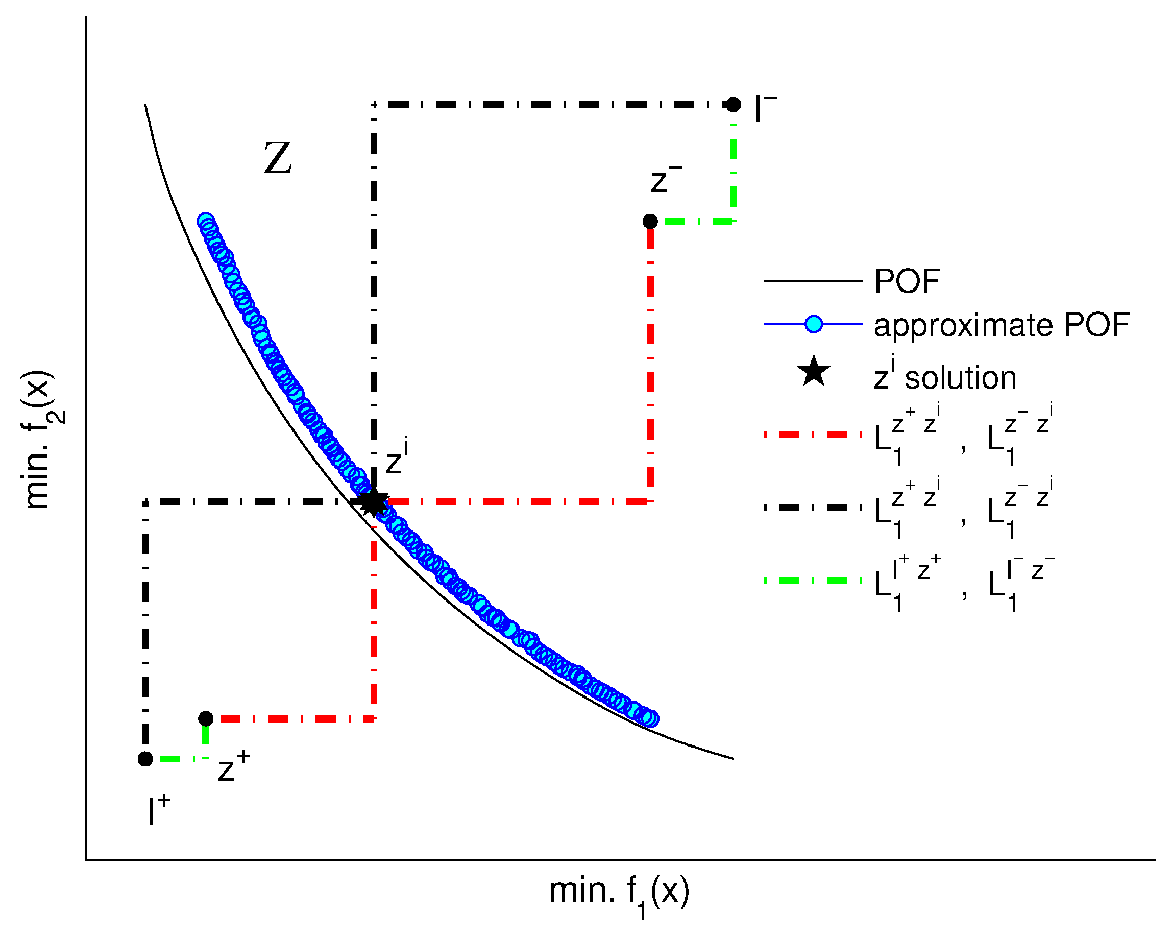
Ideal solution I + . Let us assume that only true POF of solutions are taken into account. The solution with the best possible values for each of the objective functions I + = ( I 1 + , , I j + , , I m + ) is known as the ideal solution, i.e., I j + = min. f j (x) (see Figure 1).
Nadir solution I . Let us assume that only true POF of solutions are taken into account. The solution with the worst possible values for each of the objective functions z = ( z 1 , , z j , , z m ) is known as the nadir solution, i.e., z j = max. f j ( x ) (see Figure 1).
Approximate ideal solution z + . Let us assume that only approximate POF of solutions are taken into consideration. The solution with the best possible values for each of the objective functions z + = ( z 1 + , , z j + , , z m + ) is known as the approximate-POF-based ideal solution, i.e., z j + = min. f j ( x ) (see Figure 1).
Approximate nadir solution z . Let us assume that only approximate POF of solutions are taken into account. The solution with the worst possible values for each of the objective functions z = ( z 1 , , z j , , z m ) is known as the approximate-POF-based nadir solution, i.e., z j = min. f j ( x ) (see Figure 1).
TOPSIS method. The TOPSIS method [2] establishes that the chosen solution should have the shortest distance to the ideal solution I + and the longest distance from the nadir solution I . The weighted distance of each solution from I + and I , according the chosen value p, can be, respectively, calculated as (3) and (4). Afterwards, the similarity ratio S ( z ) , defined in Equation (5), is assigned to each solution. The final ranking of solutions is obtained sorting the set of solutions decreasingly in terms of S ( z ) .
L p I + ( z ) = j = 1 m w j p z j I j + p 1 / p
L p I ( z ) = j = 1 m w j p I j z j p 1 / p
S ( z ) = L p I ( z i ) L p I + ( z i ) + L p I ( z i ) 0 S ( z ) 1

3. Methodology

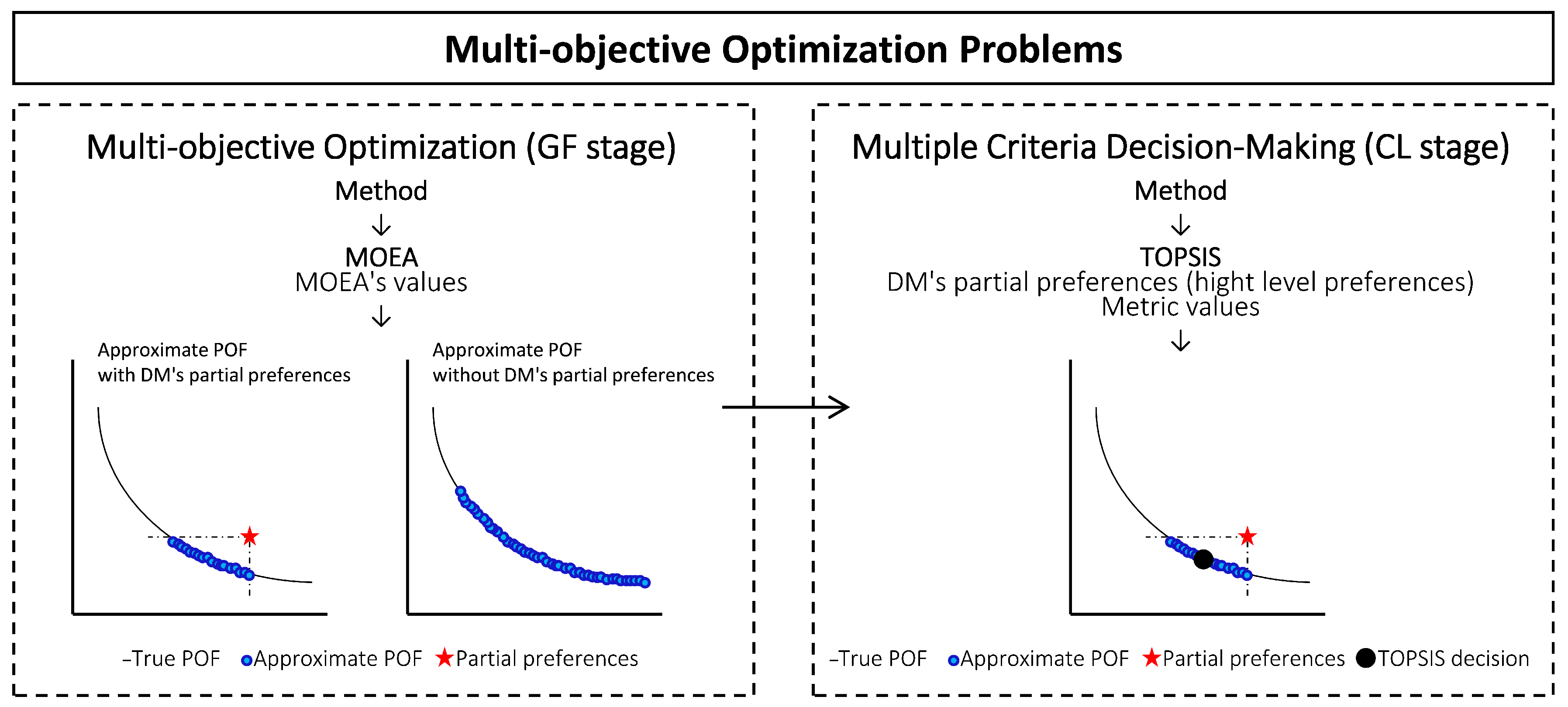
The proposed method in this article draws together two independent technical stages of MOO and MCDM, as shown in Figure 2.
Let us assume a MOP defined according to (1). Firstly, in the optimization stage (GF): (i) the DM decide which method to select to solve the MOP; and (ii) the DM specifies the parameters values of the metaheuristic algorithm used. Then, the algorithm is executed until the stopping condition has been reached. At this point, a discretized approximate POF of non-dominated solutions is available (see Figure 1) (two objective functions are considered), and the matrix formulation (6) where the POF= { z i , i = 1 , 2 , , n } of solutions is compared to the set of objective functions { z j , j = 1 , 2 , , m } according to the e i j evaluations of the solution z i regarding the objective z j .
z 1 . . z j . . z m z 1 . . z i . . z n ( e 1 1 . . e j 1 . . e m 1 . . . . . . . . . . . . . . e 1 i . . e j i . . e m i . . . . . . . . . . . . . . e 1 n . . e j n . . e m n )
Subsequently, now in the decision-making stage (CL), we proceed as follows: (i) the DM decides which method to select for choosing the preferred solution; (ii) the DM expresses weights (high-level preferences) w = { w j , j = 1 , 2 , , m } associated to each objective function and metric value; (iii) based on the discretized approximate POF of obtained solutions, the weighted distance L 1 z + to the approximate-POF-based ideal solution z + and the weighted distance L 1 z to the approximate-POF-based nadir solution z are computed for each solution (see Figure 1); and (iv) the final ranking of solutions is given by similarity ratio S * ( z i ) defined in Equation (7).
S * ( z i ) = L p z ( z i ) L p z + ( z i ) + L p z ( z i )
Proposition 1.
Using the L 1 distance metric to the approximate-POF-based ideal ( z + ) and nadir ( z ) solutions and the L 1 distance metric to the ideal ( I + ) and nadir ( I ) solutions in TOPSIS method, z i approximate POF, we obtain the same ranking of solutions.
Proof of Proposition 1.
Let us assume that the ideal I + = ( I 1 + , , I m + ) and nadir I = ( I 1 , , I m ) solutions are the true solutions of a real MOP. Using the L 1 distance in TOPSIS method, the ranking of solutions z i approximate POF can be calculated by solving (8).
S ( z i ) = L 1 I ( z i ) L 1 I + ( z i ) + L 1 I ( z i )
We consider now the distance between a solution z i and the z , z + , I , I + solutions defined in Equation (9)–(12) and the distance between the z , I solutions defined in Equation (13).
L 1 z ( z i ) = j = 1 m w j z j e j i = j = 1 m w j ( z j e j i ) = j = 1 m w j z j j = 1 m w j e j i
L 1 z + ( z i ) = j = 1 m w j e j i z j + = j = 1 m w j ( e j i z j + ) = j = 1 m w j e j i j = 1 m w j z j +
L 1 I ( z i ) = j = 1 m w j I j e j i = j = 1 m w j ( I j e j i ) = j = 1 m w j I j j = 1 m w j e j i
L 1 I + ( z i ) = j = 1 m w j e j i I j + = j = 1 m w j ( e j i I j + ) = j = 1 m w j e j i j = 1 m w j I j +
L 1 z I ¯ = j = 1 m w j I j z j = j = 1 m w j ( I j z j ) = j = 1 m w j I j j = 1 m w j z j = C 1
where C 1 is a constant.
Furthermore, when j = 1 m w j e j i is isolated and solved in (9) and subsequently replaced in (11), Equation (14) is obtained.
L 1 I ( z i ) = L 1 z ( z i ) j = 1 m w j z j + j = 1 m w j I j
If we now consider Equations (13) and (14), we obtain (15).
L 1 I ( z i ) = L 1 z ( z i ) + C 1
On the other hand, if we consider Equations (11) and (12), we have:
L 1 I + ( z i ) + L 1 I ( z i ) = j = 1 m w j I j j = 1 m w j I j + = C 2
where C 2 is a constant.
Finally, if we take into account Equations (15) and (16) and subsequently replace them in (8), we obtain (17), which implies z i approximate POF. Using the L 1 distance to the approximate-POF-based ideal ( z + ) and nadir ( z ) solutions and the L 1 distance to the ideal ( I + ) and nadir ( I ) solutions in TOPSIS method, we obtain the same ranking of solutions, even when said ideal I + and nadir I solutions are unknown. □
S ( z i ) = L 1 I ( z i ) L 1 I + ( z i ) + L 1 I ( z i ) = L 1 z ( z i ) + C 1 C 2
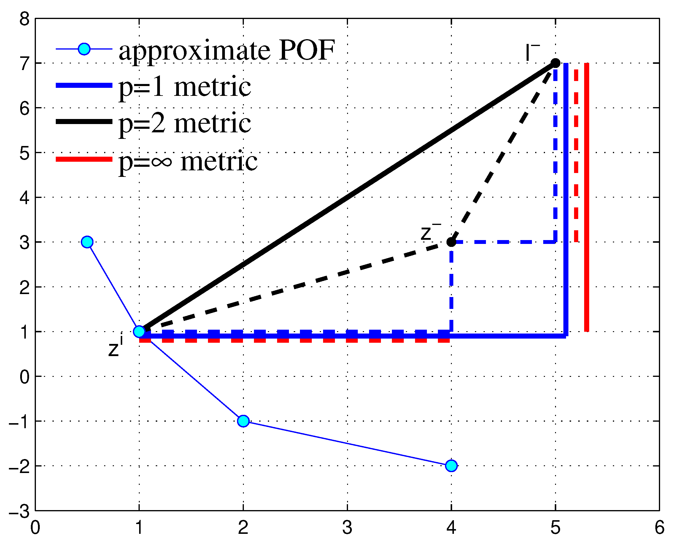
To make using Equations (9)–(17) more intuitive, Figure 3 illustrates the distances z i z ¯ , z i I ¯ and z I ¯ with p = 1 , 2 , metric. Assuming that nadir I solution is known, it can be seen that Equation (15) is satisfied (and therefore proposition 1) if, and only if p = 1 metric is used in Equations (9)–(17), find below the details of the calculation. In addition, note that, using any of the other Pareto front z i solutions, the results are similar and distance z I ¯ is a constant ( C 1 ).
p = 1 : L 1 z i z ¯ + L 1 z I ¯ = ( 3 + 2 ) + ( 1 + 4 ) = 10 = L 1 z i I ¯ = ( 4 + 6 ) = 10 p = 2 : L 2 z i z ¯ + L 2 z I ¯ = ( 3 2 + 2 2 ) + ( 1 2 + 4 2 ) = 7.73 L 2 z i I ¯ = ( 4 2 + 6 2 ) = 7.21 p = : L z i z ¯ + L z I ¯ = 3 + 4 = 7 L z i I ¯ = 6
Consequently, in convex problems, the method may be useful in providing an important clue to a DM in his/her final decision, especially when the true Pareto front of a multi-objective real-world problem is not available.
Finally, it should be highlighted that, in the proof of Proposition 1, Equations (9)–(16), all the sums go up to a value m (objectives) and the methodology is therefore clearly applicable (at stage MCDM) in many objective optimization problems.

4. Results

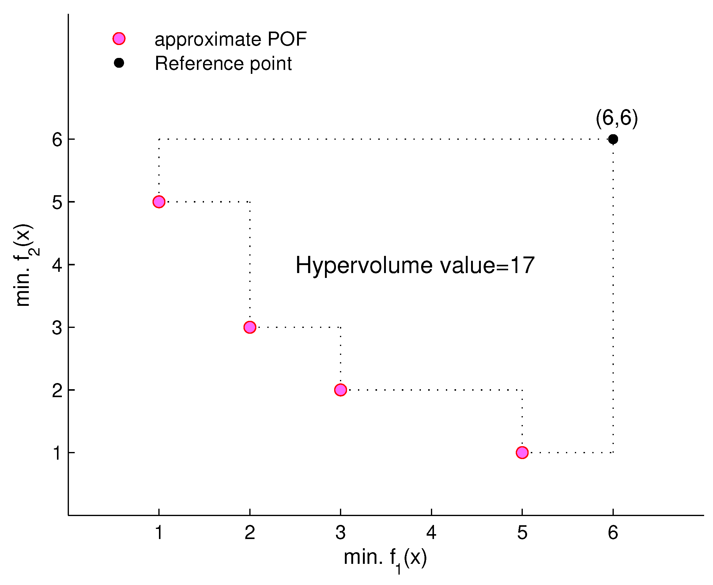
In this section, we first apply the proposed methodology in this study to the bi-objective welded beam design problem. The objectives of the design are to minimize the cost of fabrication and to minimize the deflection. This problem is well-studied in both mono- [55,56,57] and multi-objective [52,54,58,59,60] literature. In the optimization stage, the NSGA-II, GWASF-GA and MOEA/D algorithms and the g-NSGA-II and WASF-GA algorithms (that include DM’s partial-preferences as a reference point) were implemented with binary coding. In addition, tournament selection, uniform crossover and bitwise mutation were used. The crossover probability was set to 0.8 and the mutation rate to 1 / n where n = 120 is the string length; each variable (four design variables) uses 30 bits (eight decimal place precision). A population of sizes of N = 50 and N = 100 individuals and a maximum number of G = 100 generations were used. The hypervolume metric presented in [61] was used as a comparison measure between algorithms (see Figure 4). The reference point considered for the calculation of hypervolume was ( 100.0 , 0.1 ) , which guarantees that it is dominated by all the solutions generated at the end of the evolution of the algorithms. Besides, the best cost objective value obtained by the algorithms were compared in terms of statistical results and number of function evaluations (i.e., N F E s = N × G ). Each algorithm was independently run 100 times for each test instance in the same initial conditions, from a randomly generated population. In the decision-making stage, when solving Equations (7) and (8), and to avoid any influence from the scale of measurement chosen for the various objectives, the objectives were normalized [7] using the procedure z i m i n z i m a x z i m i n z i with z i approximate POF.
In a second test case, we demonstrate the utility of the suggested approach, by adding to the above mentioned problem the normal stress as a third objective function that should be minimized [54]. In this example, it was only considered the decision-making process. The TOPSIS [2] and ELECTRE I [6] methodologies were compared. In the TOPSIS and ELECTRE I approaches, equal weights values were assigned to all objective functions. Besides, a set of non-dominated solutions obtained in a randomized trial of NSGA-II ( N = 50 , G = 500 ) was used for comparisons.

4.1. Bi-Objective Welded Beam Design Problem (Optimization)

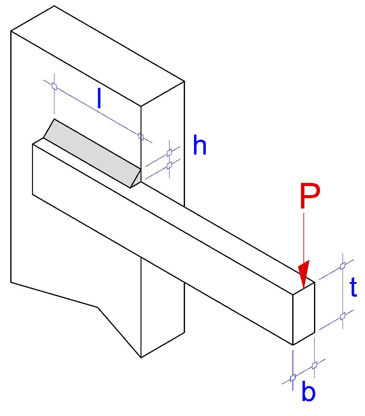
This design problem [58] minimizes both the cost and the deflection due to load P. The two objectives conflict since minimizing deflection will lead to an increase in manufacturing cost, which mainly includes the set-up cost, material cost and welding labor cost. The design involves four different design decision variables ( h , l , t , b ) (see Figure 5) and four nonlinear constraints: shear stress, normal stress, weld length and the buckling limitation. Formally, the bi-objective welded beam design problem can be defined as follows:
m i n . f 1 ( x ) = 1.10471 h 2 l + 0.04811 t b ( 14.0 + l ) m i n . f 2 ( x ) = δ ( x ) = 2.1952 t 3 b s . t . g 1 ( x ) = 13600 τ ( x ) 0 g 2 ( x ) = 30000 σ ( x ) 0 g 3 ( x ) = b h 0 g 4 ( x ) = P c ( x ) 6000 0 h , b [ 0.125 , 5 ] l , t [ 0.1 , 10 ] w h e r e τ ( x ) = ( τ ( x ) ) 2 + ( τ ( x ) ) 2 + l τ ( x ) τ ( x ) 0.25 ( l 2 + ( h + t ) 2 ) τ ( x ) = 6000 2 h l τ ( x ) = 6000 ( 14 + 0.5 l ) 0.25 ( l 2 + ( h + t ) 2 ) 2 0.707 h l ( l 2 / 12 + 0.25 ( h + t ) 2 ) P c ( x ) = 64746.022 ( 1 0.0282346 t ) t b 3 σ ( x ) = 504000 t 2 b
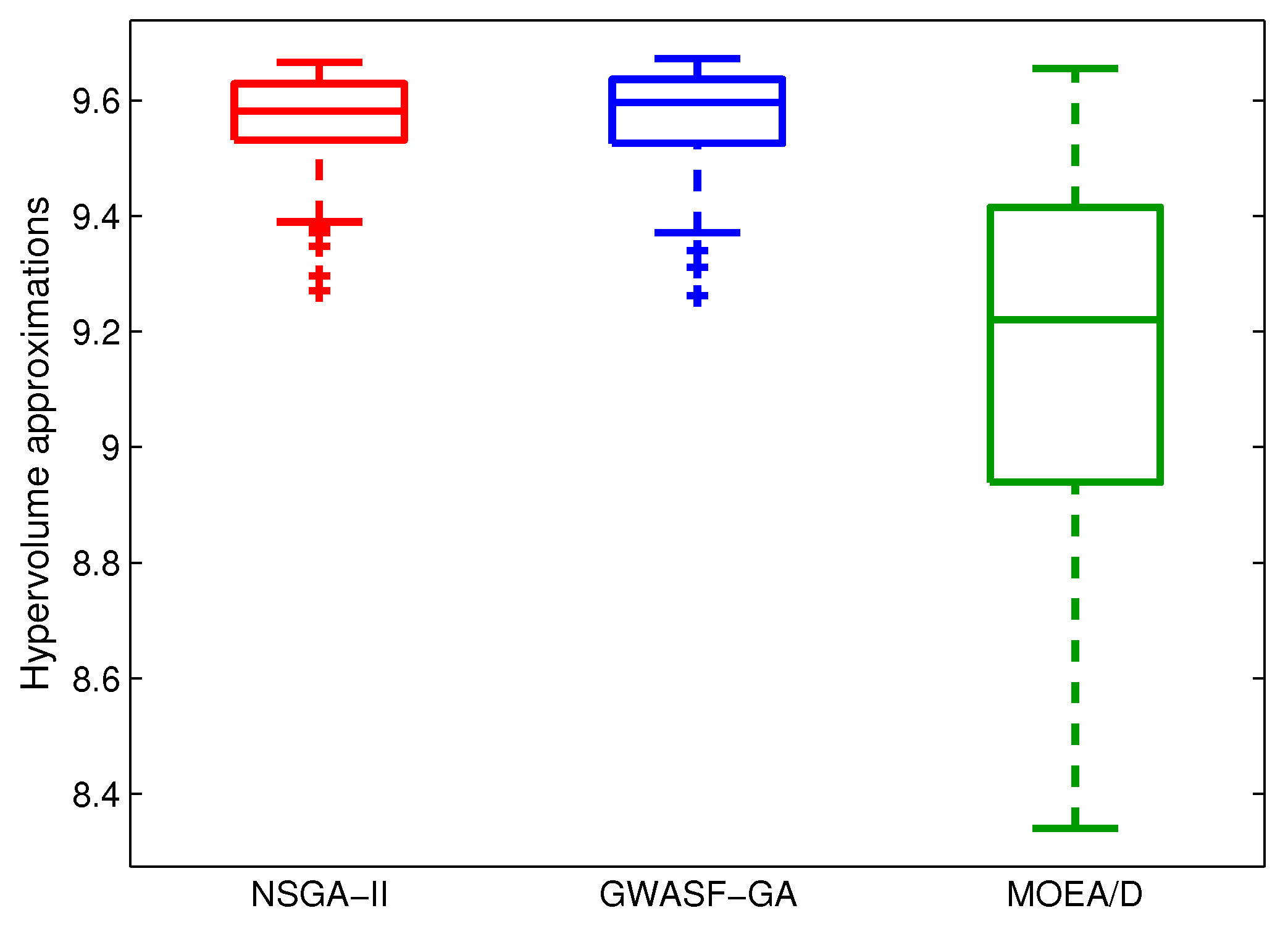
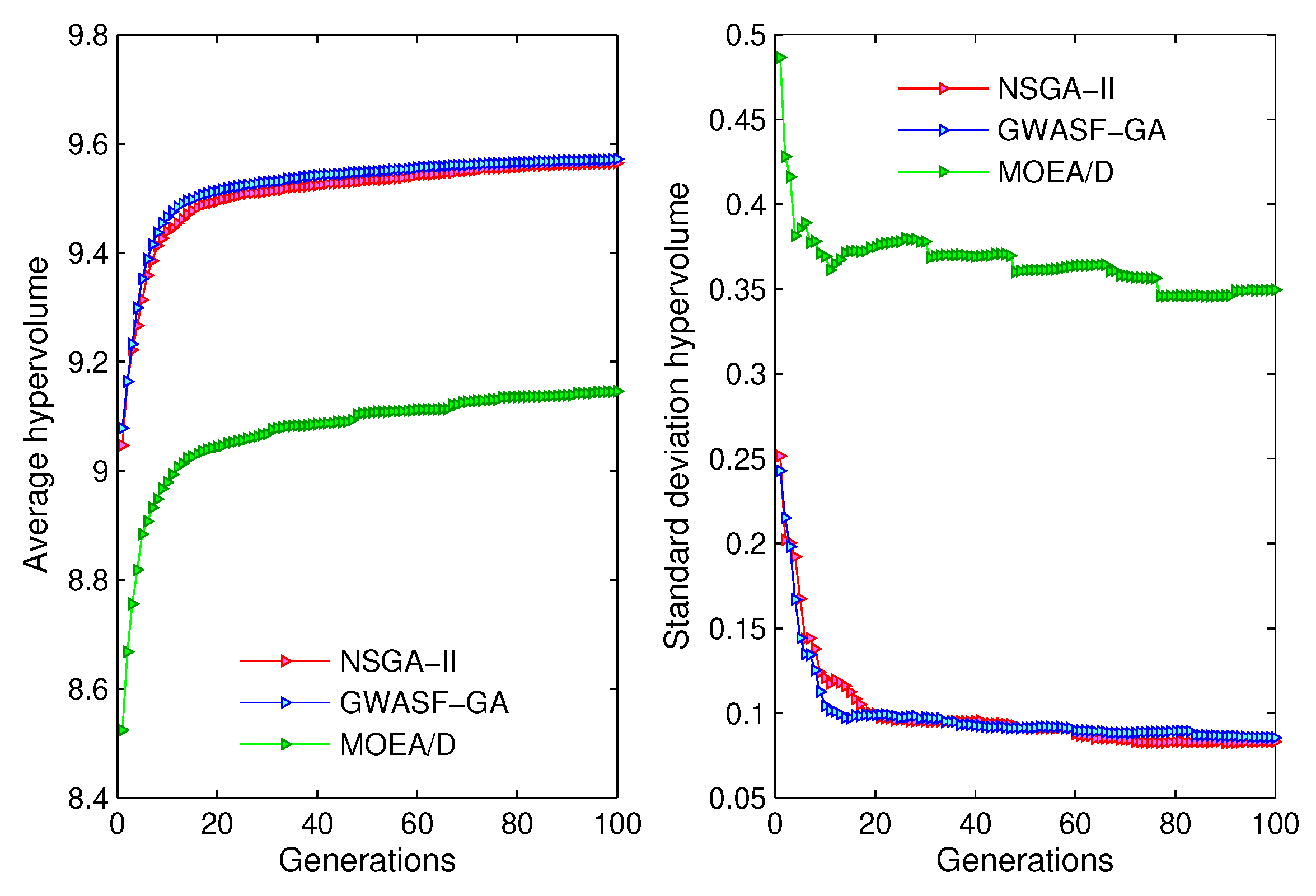
Firstly, NSGA-II, GWASF-GA and MOEA/D (other metaheuristic methods could have been used) were used to find the approximate Pareto fronts and then compared the results using the hypervolume metric. Table 1 shows the mean, standard deviation, best and worst hypervolume indicators achieved, over 100 independent runs. It can be seen that the NSGA-II and GWASF-GA algorithms attain the best performance. Figure 6 and Figure 7 show a more detailed comparison between the algorithms from Table 1 with N = 100 and G = 100 . Figure 6 shows the box plots based on the hypervolume approximation metric. We can see that the best median value and the lowest dispersion value are obtained with NSGA-II and GWASF-GA. In addition, in Figure 7 (left) that presents the evolution of the average hypervolume per generation and in Figure 7 (right) that shows the evolution of the standard deviation hypervolume, it is observed that the NSGA-II and GWASF-GA algorithms obtain similar values which are significantly better than the values achieved by MOEA/D.
Moreover, various MOEAs have been applied to the problem (18) by different researchers. Table 2 shows the statistical results of the best objective cost, the mean value and the standard deviation value obtained in this work with NSGA-II ( N F E s = 5000 and 10,000), GWASF-GA ( N F E s = 5000 and 10,000) and MOEA/D ( N F E s = 5000 and 10,000) with those attained by other bi-objective metaheuristics. It can see that GWASF-GA ( N F E s = 10,000) has the best objective cost followed by NSGA-II ( N F E s = 10,000) and MOWCA ( N F E s = 15,000). In addition, it can be noted in Table 2 that GWASF-GA with N F E s = 10,000 ( N = 100 and G = 100 ) reaches the best mean value ( 3.5657 ).
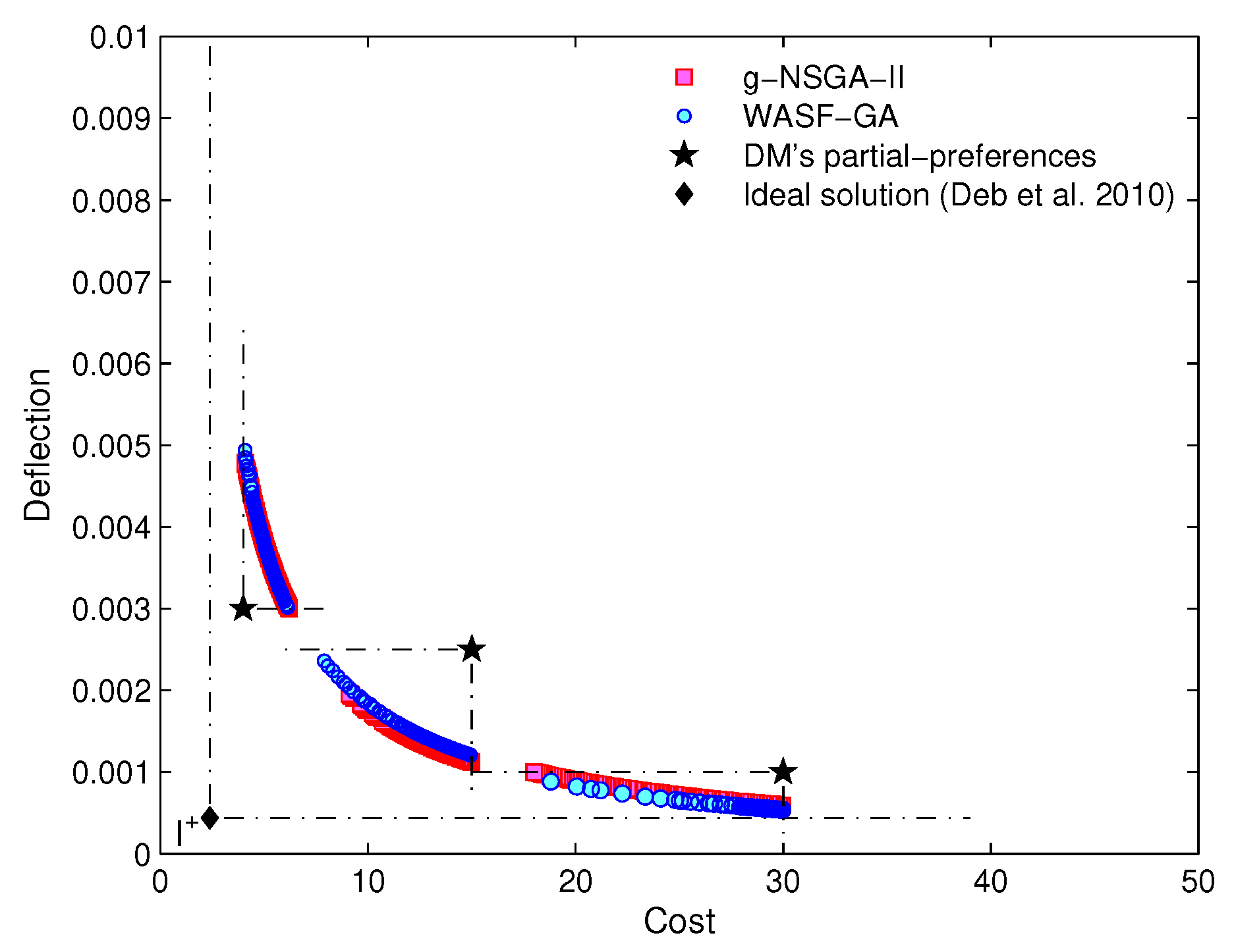
Secondly, a similar study to the previous one using the g-NSGA-II and WASF-GA algorithms (although other metaheuristic methods with DM’s partial-preferences could have been used) was performed considering three different reference points (DM’s partial-preferences) ( 4 , 0.003 ) , ( 15 , 0.0025 ) and ( 30 , 0.001 ) , infeasible and feasible (see Figure 8). The hypervolume metric of the region of interest defined in [43] was used as a comparison measure for the two algorithms.
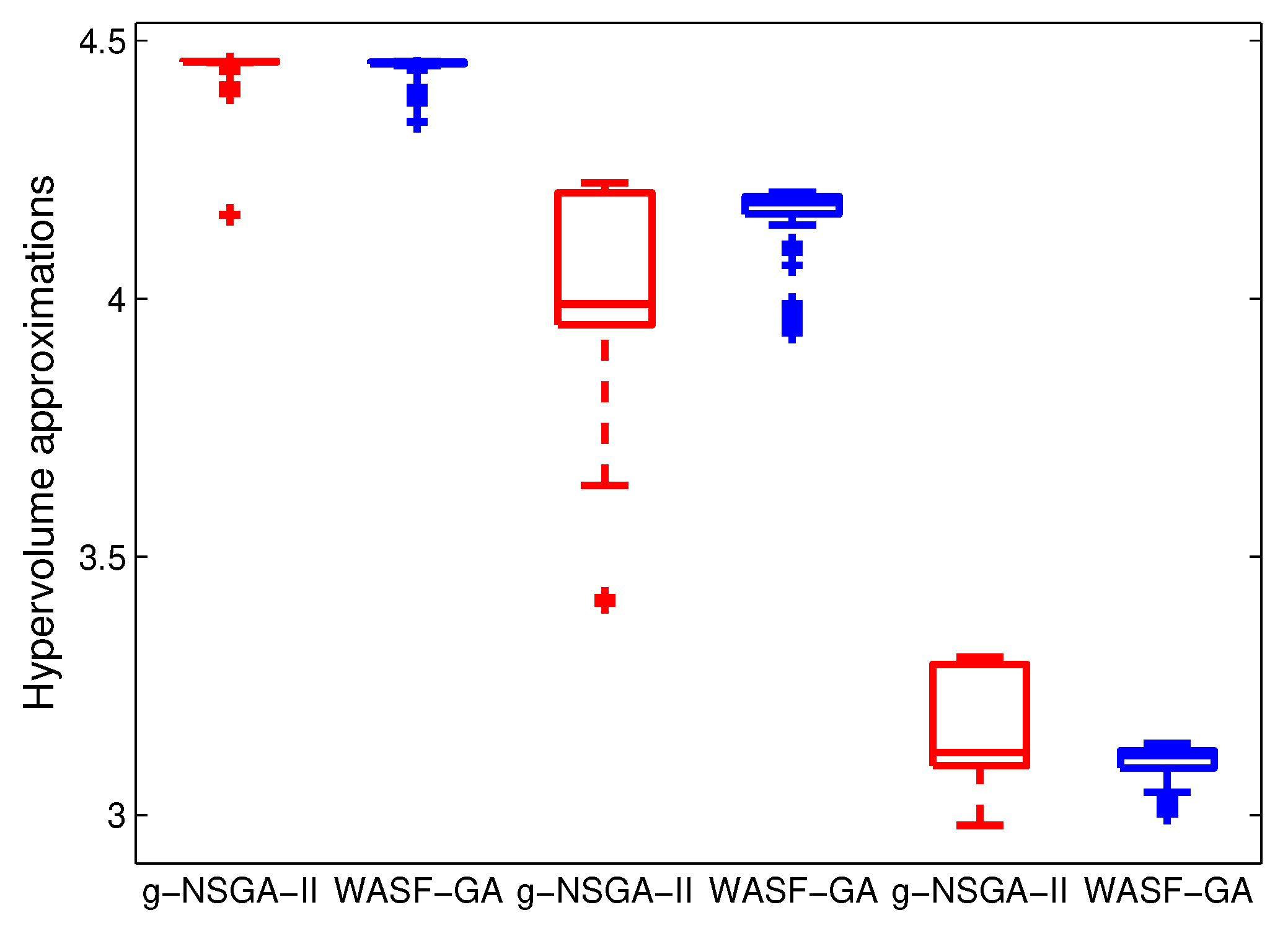
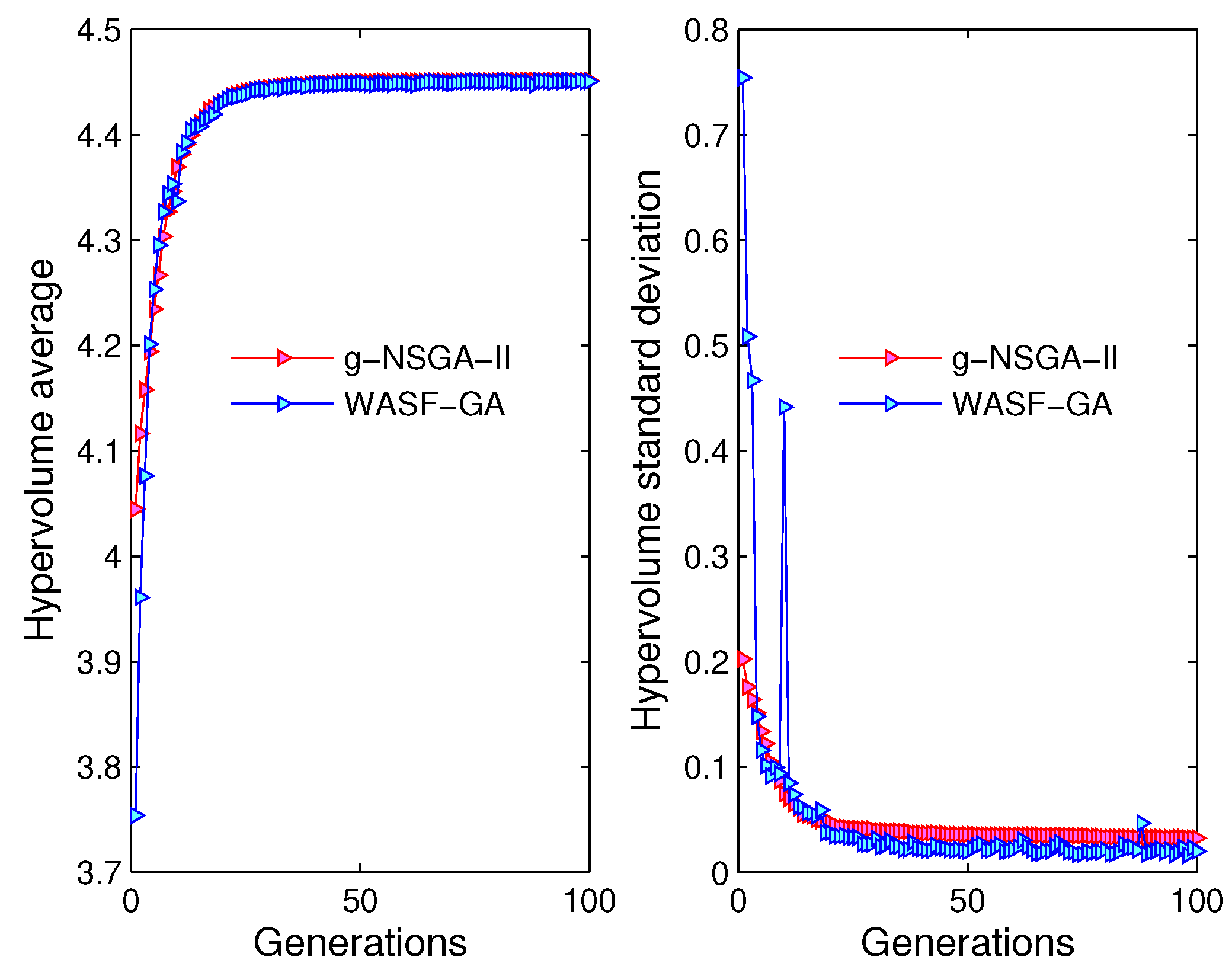
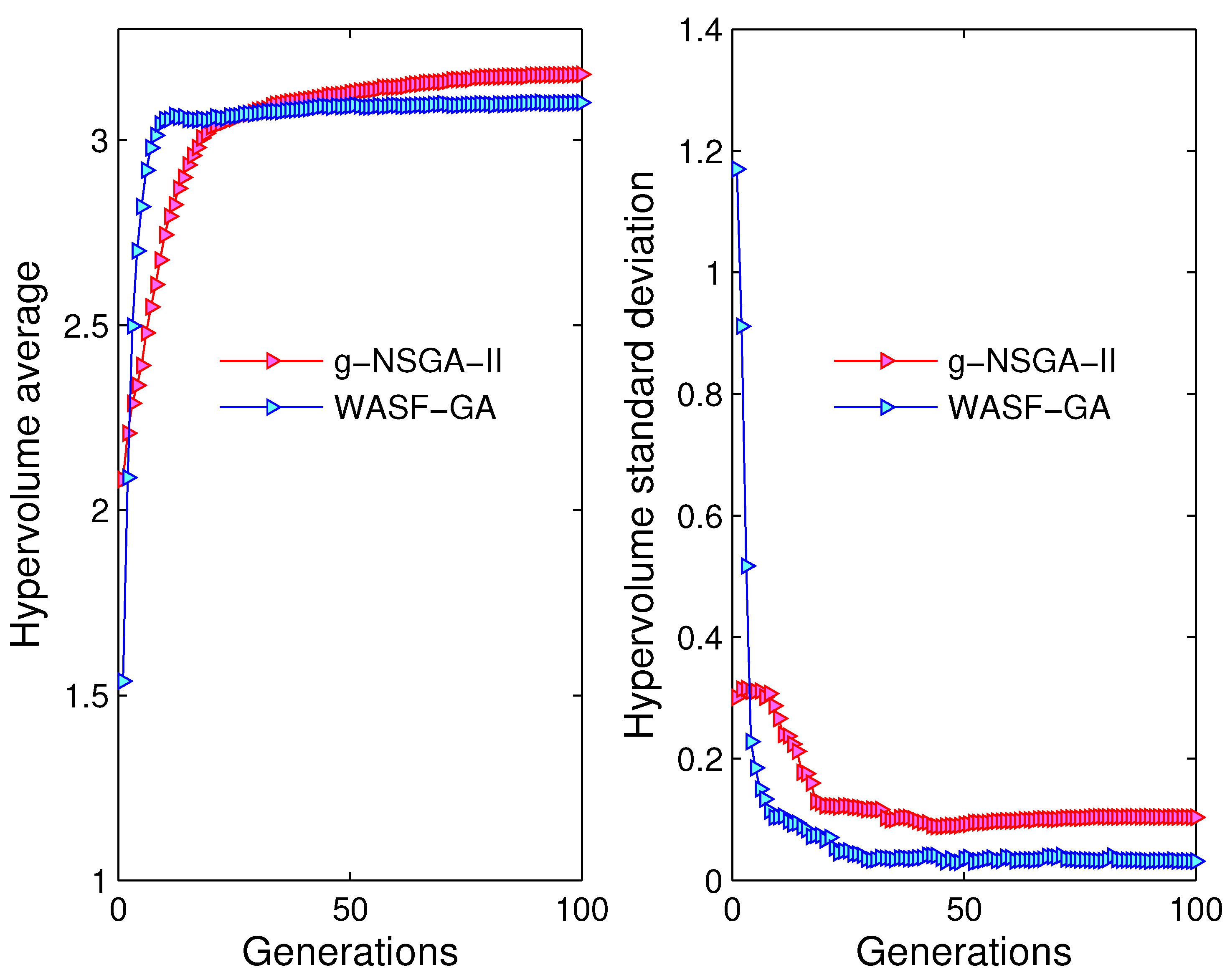
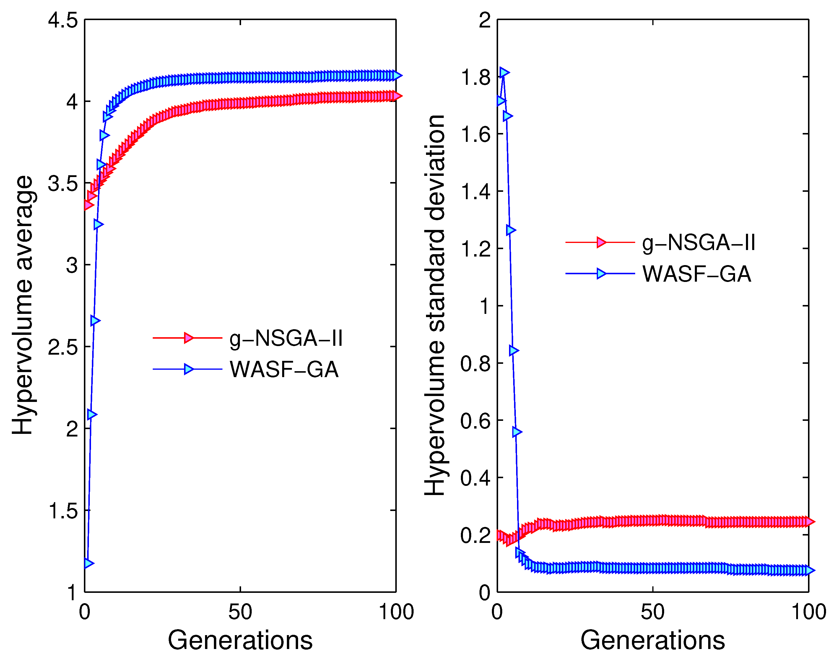
Table 3 presents the mean, standard deviation, best and worst hypervolume indicators achieved, over 100 independent runs, by the g-NSGA-II and WASF-GA algorithms. It can be perceived that the values obtained can be quite different depending on the reference point used. For example, when the reference point was set to ( 4 , 0.003 ) (non-feasible), the performances obtained for both, g-NSGA-II and WASF-GA, were similar (see also Figure 8, Figure 9 and Figure 10). On the other hand, when the reference point was ( 30 , 0.001 ) (feasible), g-NSGA-II and WASF-GA also had similar results, although g-NSGA-II had a slightly better performance of the hypervolume metric (Figure 11 and Table 3) and better distribution of the approximate Pareto front’s solution set (Figure 8). However, the values in Table 3 show that the WASF-GA algorithm obtained superior performance than g-NSGA-II when the reference point was set to ( 15 , 0.0025 ) (see also Figure 8, Figure 9 and Figure 12).

Bi-Objective Welded Beam Design Problem (Decision)

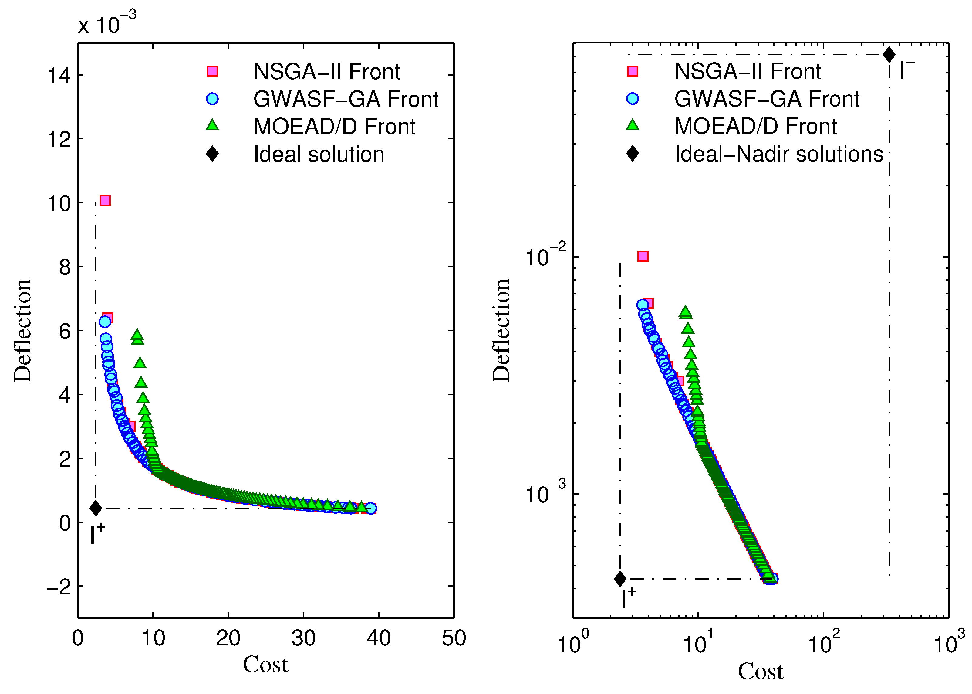
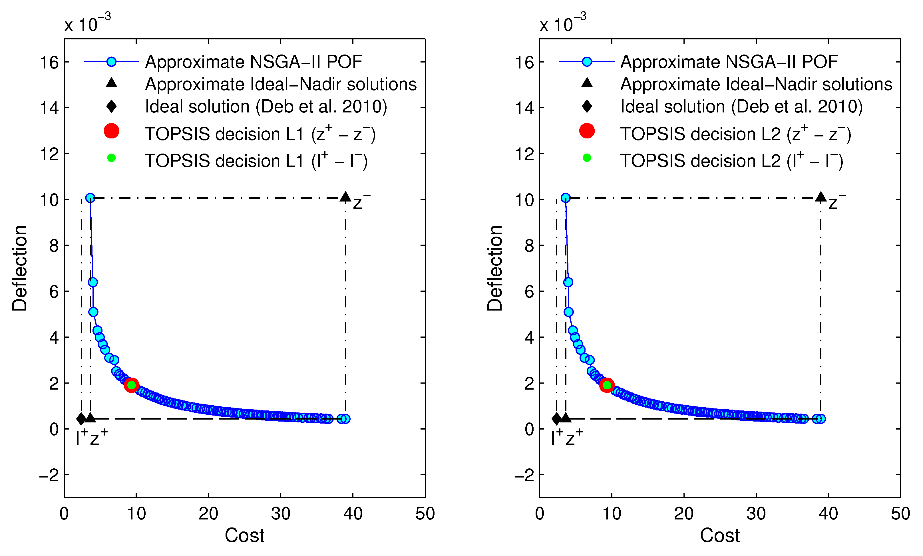
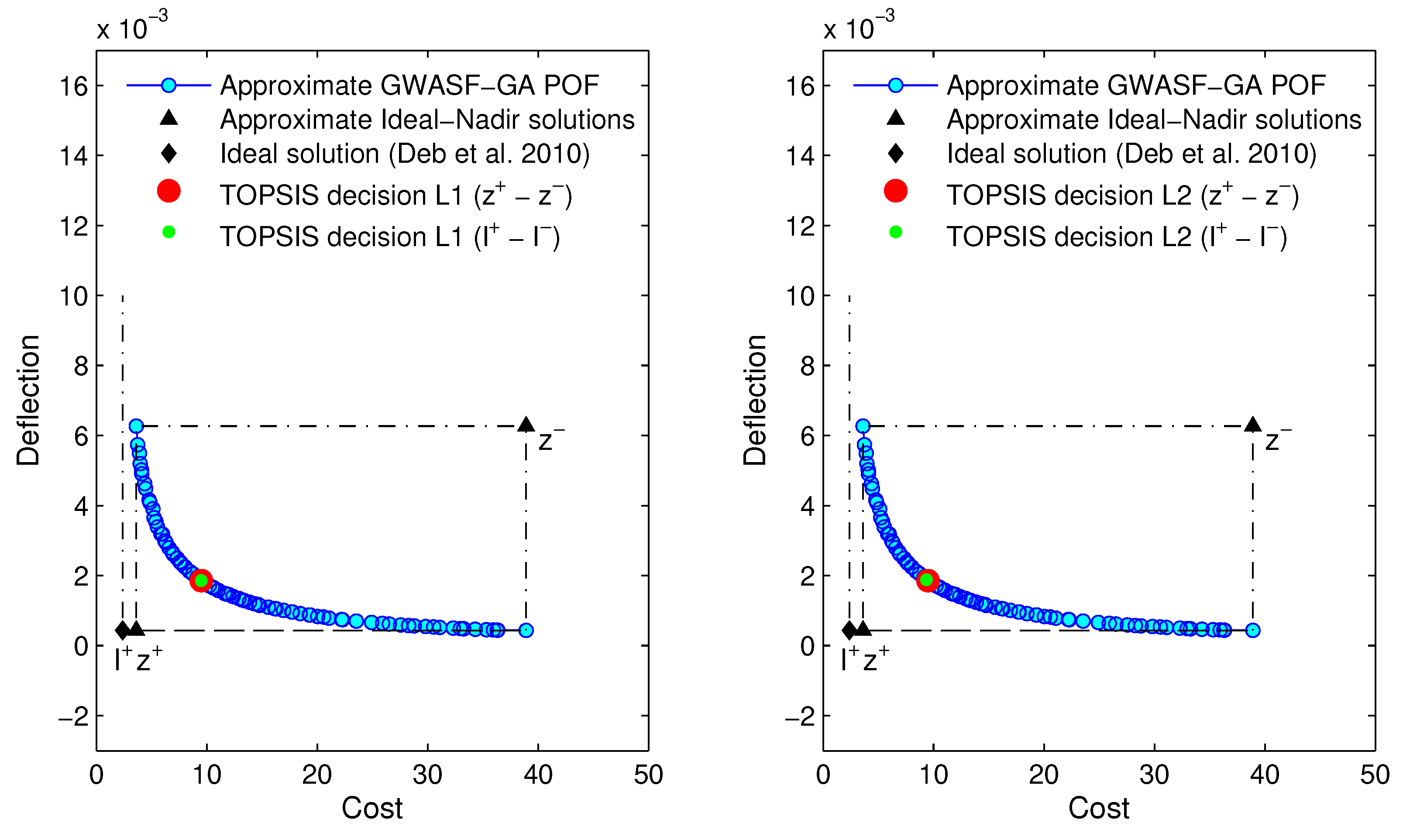
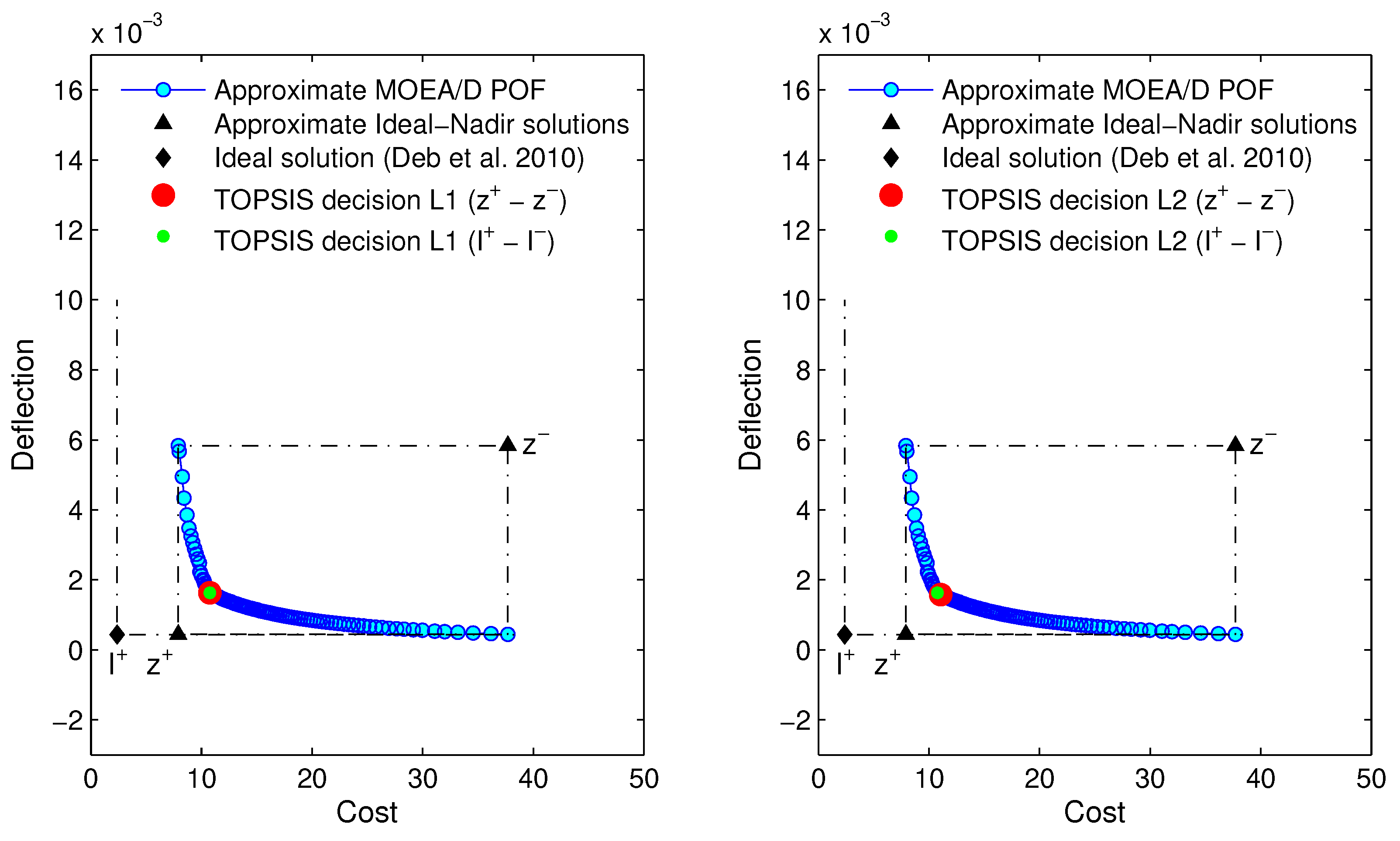
In this section, the second stage (CL) is executed. Now, TOPSIS (other method supporting DM could have been used) is used to rank the solutions and to determine the best TOPSIS decision (rank-1 solution). The L 1 and L 2 metrics in TOPSIS model were utilized. In addition, the approximate Pareto front with the hypervolume indicator closest to the average value of hypervolume after 100 runs was adopted for comparisons and for each algorithm (see Figure 13, left and right (with logarithmic scale to appreciate de nadir solution)). As expected, the appearance of the approximate set of Pareto optimal solutions changes with the trial and the employed algorithm. Therefore, the choice of the DM is conditioned by the quality of the POF achieved. The best known ideal and nadir values ( 2.3810 , 0.000439 ) and ( 333.9095 , 0.0713 ) , respectively [54], of the problem (18) were used in the experiments (see Figure 13, right).
First, POF resulting from the NSGA-II, GWASF-GA and MOEA/D algorithms were considered. Table 4 and Table 5 give the eight best solutions ranked from best to worst. The first two columns represent the coordinates of the solutions in the objective space, the third and fourth columns give the distances of the solutions regarding the z + and z and the I + and I solutions, the fifth column gives the similarity values S z + z and S I + I according TOPSIS method and the last two columns show the ranking of solutions regarding both the z + and z and the I + and I solutions. The results in Table 4 show that, by using L 1 metric in the TOPSIS model, with respect to both the ideal z + and nadir z solutions of the approximate POF obtained by the algorithms and the I + and I solutions of the real POM, the ranking of the proposal solutions bears the same ranking. However, when L 2 metric is used, the ranking of the proposed solutions differs (see the last two columns of the Table 5).
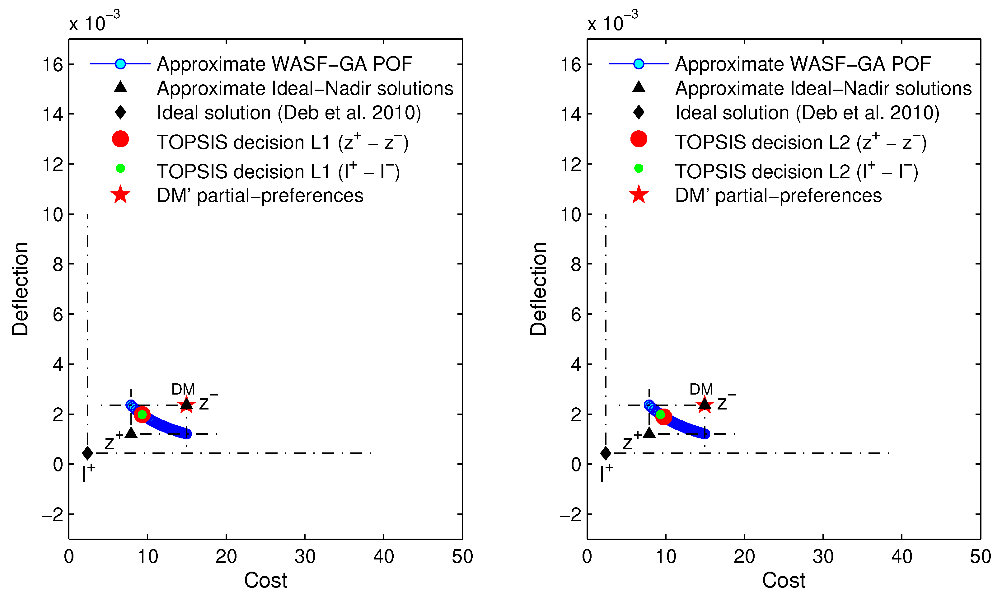
Note that the best solution (rank-1) is referred to in this paper as the TOPSIS decision. Logically, this solution does not change when L 1 metric is used (see Figure 14, Figure 15 and Figure 16 (left) and Table 4). Nevertheless, this is not always the case when using the metric L 2 (see Figure 14, Figure 15 and Figure 16 (right) and Table 5).
Finally, when DM’s partial-preferences were introduced into the algorithms, the results were very similar to those presented above. In order not to be redundant, only WASF-GA results (DM’s partial-preferences: 15 , 0.0025 ) are shown. The results of the last two columns of Table 6 show that, by using L 1 metric in the TOPSIS model, the ranking of the proposal solutions bears the same ranking. However, when L 2 metric is used, the ranking of the proposed solutions differs (see the last two columns of Table 7). Figure 17 (left) also shows that the TOPSIS decision (rank-1 solution) does not change when L 1 metric is used, and this is not the case when using the metric L 2 (Figure 17, right).

4.2. Three-Objective Welded Beam Design Problem (Decision)

In this section, problem (18) is redefined considering normal stress σ ( x ) as a third objective function to be minimized. The new mathematical description of the problem [54] is formulated below. By including normal stress as a third objective, the decision-making process in the objective space is even more difficult (see Figure 18).
m i n . f 1 ( x ) = 1.10471 h 2 l + 0.04811 t b ( 14.0 + l ) m i n . f 2 ( x ) = δ ( x ) = 2.1952 t 3 b m i n . f 3 ( x ) = σ ( x ) = 504000 t 2 b s . t . g 1 ( x ) = 13600 τ ( x ) 0 g 2 ( x ) = 30000 σ ( x ) 0 g 3 ( x ) = b h 0 g 4 ( x ) = P c ( x ) 6000 0 h , b [ 0.125 , 5 ] l , t [ 0.1 , 10 ] w h e r e τ ( x ) = ( τ ( x ) ) 2 + ( τ ( x ) ) 2 + l τ ( x ) τ ( x ) 0.25 ( l 2 + ( h + t ) 2 ) τ ( x ) = 6000 2 h l τ ( x ) = 6000 ( 14 + 0.5 l ) 0.25 ( l 2 + ( h + t ) 2 ) 2 0.707 h l ( l 2 / 12 + 0.25 ( h + t ) 2 ) P c ( x ) = 64746.022 ( 1 0.0282346 t ) t b 3
In this problem, the methodology proposed in this paper was implemented in the following way. After a set of Pareto-optimal solutions was obtained by a MOEA (a set of potential solutions obtained in a randomized trial of NSGA-II with N = 50 and G = 500 was used for comparisons, see Figure 18), the TOPSIS and ELECTRE I methodologies were used to determine the most attractive solution for a DM. The results shown in Table 8 and Table 9 do not differ much from those obtained for the problem (18) with two objective functions. With respect to both the ideal z + and nadir z solutions and the I + and I solutions, the ranking of solutions does not change if the L 1 metric is used in the TOPSIS method; this cannot be stated for using L 2 metric.
Finally, a study using the ELECTRE I method is included in this section. In a first step, all data (see Columns 1–3 of Table 8 or Table 9 showing eight values out of fifty) were normalized, and equal weights values were assigned to all objective functions. Then, the concordance and discordance coefficients for all the pairs of solutions, according to the authors of [7,16], were calculated to obtain the concordance matrix and discordance matrix. To finish, the aggregate dominance matrix (50 × 50) (Table 10) was determinate by setting the threshold c ¯ for the concordance test to 0.1 and the threshold d ¯ for the non-discordance test to 0.9. From the results in Table 10, it can be said that Solution 33 (9.22674, 0.00194, 4446.90136) (cost, deflection and normal stress, respectively) is better than all the others. A sensitivity analysis of the c ¯ and d ¯ values was carried out, and it was found that Solution 33 (9.226740, 0.001943, 4446.901367) is always represented (see Table 11).
To conclude, the values of the solutions calculated by TOPSIS and ELECTRE I are shown numerically in Table 12 and graphically in Figure 18. Table 12 shows that ELECTRE I obtained a lower value of the cost function than obtained by TOPSIS. However, lower deflection and normal stress values were achieved by TOPSIS. Besides, with the L 1 metric, as demonstrated in Section 3, TOPSIS guarantees that the proposed solution is classified with respect to both the ideal I + and nadir I solutions even if these are not known. It could also be deduced from the results in Figure 18 that the solution achieved by ELECTRE I resides or is close to a knee region [62,63,64,65,66,67,68] where a small improvement in one of the objectives leads to a significant degradation in at least one of the other objectives, and therefore it may be of more interest to a DM than the solution calculated by TOPSIS. In any case, the selection of the best MCDM method for a given problem can be a difficult task [69], and it is not within the scope of this work.

5. Conclusions

Usually in the literature of Multi-objective Metaheuristics (MOMH), the background on Multiple Criteria Decision-Making is ignored. This work is so rich not only in the classical aspects of MOMH but also in the MCDM. In this context, this paper proposes and demonstrates the effectiveness of a search procedure that brings together two independent technical stages of MOO and MCDM.
In the optimization stage, a variety of representative a posteriori algorithms, NSGA-II, GWASF-GA and MOEA/D, and with DM’s partial-preferences, g-NSGA-II and WASF-GA, were used during the optimization process, in order to obtain an approximate Pareto-optimal Front. An original comparison of results based on hypervolume metric were performed on a welded beam engineering design referent problem (two objective functions). This problem is characterized because there is no knowledge of the ideal and nadir solutions. The obtained results clearly indicate that the NSGA-II and GWASF-GA algorithms achieved similar and better performances than those obtained by the MOEA/D algorithm. In addition, NSGA-II and GWASF-GA obtained the best results compared to other metheuristic methods of the literature. When partial preferences were introduced into the algorithms, the results of the comparisons between g-NSGA-II and WASF-GA were different depending on the used reference point (DM’s partial-preferences). When the reference point was set to ( 15 , 0.0025 ) (feasible) (towards the POF area corresponding to well-balanced solutions), the best result was obtained by WASF-GA. When the reference point was ( 30 , 0.001 ) (feasible), g-NSGA-II and WASF-GA achieved similar results, although g-NSGA-II had a slightly better performance of the hypervolume metric and better distribution of the approximate Pareto solution set. Finally, when the reference point was set to ( 4 , 0.003 ) (no-feasible), the performances were similar for both algorithms.
In the decision analysis stage, the TOPSIS methodology is proposed. Although this method requires knowledge of the ideal and nadir solutions of the MOP, in this work only approximate Pareto-optimal fronts are studied and, therefore, the ideal and nadir solutions may not be known. However, in this paper, it is shown that, by using the L 1 distance metric in the TOPSIS method, the classification of the proposed solutions has the same range. This is valid with respect to both the ideal and nadir solutions of the approximate POF obtained by the algorithms, and the true ideal and nadir solutions of the POM. This cannot be stated by using L 2 metric. For demonstration, a comparison of L 1 and L 2 metrics in TOPSIS model was performed for the studied bi-objective welded beam problem. Finally, a comparison (three objective functions) of the solutions proposed by TOPSIS and ELECTRE I was carried out. The results show that a lower value of the cost function was obtained by ELECTRE I. However, lower deflection and normal stress values were achieved by TOPSIS.
In our opinion, the proposed methodology in this work is a suggestive method for problems similar to the one studied in this paper and it may be a useful tool and provide an important clue to a DM in his/her final decision.

Author Contributions

All authors have contributed equally to the realization of this work. M.M., M.F., F.M. and R.A.-C. participated in the conception and design of the work; M.M., M.F., F.M. and R.A.-C. reviewed the bibliography; M.M., M.F., F.M. and R.A.-C. conceived and designed the experiments; M.M., M.F., F.M. and R.A.-C. performed the experiments; M.M., M.F., F.M. and R.A.-C. analyzed the data; and M.M., M.F., F.M. and R.A.-C. wrote and edited the paper. All authors have read and agreed to the published version of the manuscript.

Funding

This research received no external funding.

Acknowledgments

This work was possible thanks to the collaboration and support of the University Institute of Intelligent Systems and Numeric Applications in Engineering (IUSIANI-ULPGC).

Conflicts of Interest

The authors declare no conflict of interest.

Abbreviations

The following abbreviations are used in this manuscript:
MOPMulti-Objective Optimization Problem
MCDMMultiple Criteria Decision-Making
MOOMulti-Objective Optimization
MOMHMulti-Objective Metaheuristic
DMHuman Decision-Maker
POFPareto-Optimal front
MOEAMulti-Objective Evolutionary Algorithm
GFCLGenerate First–Choose Later
NSGA-IINon-Dominated Sorting Genetic Algorithm-II
MOEA/DMulti-Objective Evolutionary Algorithm based on Decomposition
GWASF-GAGlobal Weighting Achievement Scalarizing Function Genetic Algorithm
WASF-GAWeighting Achievement Scalarizing Function Genetic Algorithm
g-NSGA-IINon-g-Dominated Sorting Genetic Algorithm
NFEsNumber of Function Evaluations
TOPSISTechnique for Order Preference by Similarity to an Ideal Solution
ELECTREELimination Et Choix Traduisant la REalité
ODEMOOrthogonal Differential Evolution for Multiobjective Optimization
MOWCAMulti-Objective Water Cycle Algorithm
M2O-CSAMulti-Objective Orthogonal Opposition-Based Crow Search Algorithm
MOCSAMulti-Objective Crow Search Algorithm
MOCCSAMulti-Objective Chaotic Crow Search Algorithm
ANNArtificial Neural Network
MOMPCMulti-objective Model Predictive Control

References

  1. Saaty, T.L. The Analytic Hierarchy Process; McGraw-Hill: New York, NY, USA, 1980. [Google Scholar]
  2. Hwang, C.-L.; Yoon, K. Multiple Attribute Decision Making. Methods and applications: A state-of-the-art survey. In Lecture Notes in Economics and Mathematical Systems; Springer: New York, NY, USA, 1981; Volume 186. [Google Scholar]
  3. Jacquet-Lagreze, E.; Siskos, J. Assessing a set of additive utility functions for multicriteria decision making, the UTA method. Eur. J. Oper. Res. 1982, 10, 151–164. [Google Scholar] [CrossRef]
  4. Brans, J.P.; Vincke, P. A preference ranking organisation method: (The PROMETHEE method for multiple criteria decision-making). Manag. Sci. 1985, 31, 647–656. [Google Scholar] [CrossRef] [Green Version]
  5. Bana e Costa, C.A.; Vansnick, J.-C. General overview of the MACBETH approach. In Advances in Multicriteria Analysis; Pardalos, P.M., Siskos, Y., Zopounidis, C., Eds.; Springer: Boston, MA, USA, 1995; pp. 93–100. [Google Scholar]
  6. Roy, B. Multicriteria Methodology for Decision Aiding; Kluwer Academic Publishers: Dordrech, The Netherlands, 1996. [Google Scholar]
  7. Pomerol, J.; Barba-Romero, S. Multicriterion Decision in Management: Principles and Practices; Kluwer Academic: Norwell, MA, USA, 2000. [Google Scholar]
  8. Opricovic, S.; Tzeng, G.H. Compromise solution by MADM methods: A comparative analysis of VIKOR and TOPSIS. Eur. J. Oper. Res. 2004, 156, 445–455. [Google Scholar] [CrossRef]
  9. Tzeng, G.-H.; Huang, J.-J. Multiple Attribute Decision Making. Methods and Applications; Chapman and Hall/CRC: New York, NY, USA, 2011. [Google Scholar]
  10. Rezaei, J. Best-worst multi-criteria decision-making method. Omega 2015, 53, 49–57. [Google Scholar] [CrossRef]
  11. Vinogradova, I. Multi-Attribute Decision-Making Methods as a Part of Mathematical Optimization. Mathematics 2019, 7, 915. [Google Scholar] [CrossRef] [Green Version]
  12. Mi, X.; Tang, M.; Liao, H.; Shen, W.; Lev, B. The state-of-the-art survey on integrations and applications of the best worst method in decision making: Why, what, what for and what’s next? Omega 2019, 87, 205–225. [Google Scholar] [CrossRef]
  13. Chou, T.-Y.; Chen, Y.-T. Applying Fuzzy AHP and TOPSIS Method to Identify Key Organizational Capabilities. Mathematics 2020, 8, 836. [Google Scholar] [CrossRef]
  14. Charnes, A.; Cooper, W.W.; Ferguson, R.O. Optimal estimation of executive compensation by linear programming. Manag. Sci. 1955, 1, 138–151. [Google Scholar] [CrossRef]
  15. Zeleny, M. Compromise Programming. In Multiple Criteria Decision Making; Cochrane, J.L., Zeleny, M., Eds.; University of South Carolina Press: Columbia, SC, USA, 1973; pp. 262–301. [Google Scholar]
  16. Collette, Y.; Siarry, P. Multiobjective Optimzation: Principles and Case Studies. Computational Science & Engineering; Springer: Heidelberg, Germany, 2004. [Google Scholar]
  17. Chang, K.-H. Multiobjective Optimization and Advanced Topics. In Design Theory and Methods Using CAD/CAE; Chang, K.-H., Ed.; Academic Press: Cambridge, UK, 2015; pp. 325–406. [Google Scholar]
  18. Cui, Y.; Geng, Z.; Zhu, Q.; Han, Y. Review: Multi-objective optimization methods and application in energy saving. Energy 2017, 125, 681–704. [Google Scholar] [CrossRef]
  19. Gunantara, N. A review of multi-objective optimization: Methods and its applications. Cogent Eng. 2018, 5, 1–16. [Google Scholar] [CrossRef]
  20. Yang, X.S. Nature-Inspired Metaheuristic Algorithms; Luniver Press: Bristol, UK, 2008. [Google Scholar]
  21. Ugolotti, R.; Sani, L.; Cagnoni, S. What Can We Learn from Multi-Objective Meta-Optimization of Evolutionary Algorithms in Continuous Domains? Mathematics 2019, 7, 232. [Google Scholar] [CrossRef] [Green Version]
  22. Sun, Y.; Gao, Y. A Multi-Objective Particle Swarm Optimization Algorithm Based on Gaussian Mutation and an Improved Learning Strategy. Mathematics 2019, 7, 148. [Google Scholar] [CrossRef] [Green Version]
  23. Zhou, Y.; Wang, J.; Wu, Z.; Wu, K. A multi-objective tabu search algorithm based on decomposition for multi-objective unconstrained binary quadratic programming problem. Knowl.-Based Syst. 2018, 141, 18–30. [Google Scholar] [CrossRef]
  24. Coronado de Koster, O.A.; Domínguez-Navarro, J.A. Multi-Objective Tabu Search for the Location and Sizing of Multiple Types of FACTS and DG in Electrical Networks. Energies 2020, 13, 2722. [Google Scholar] [CrossRef]
  25. Amine, K. Multiobjective Simulated Annealing: Principles and Algorithm Variants. Adv. Oper. Res. 2019, 2019, 8134674. [Google Scholar] [CrossRef]
  26. Cunha, M.; Marques, J. A New Multiobjective Simulated Annealing Algorithm—MOSA-GR: Application to the Optimal Design of Water Distribution Networks. Water Resour. Res. 2020, 56. [Google Scholar] [CrossRef]
  27. Deb, K. Multi-Objective Optimization Using Evolutionary Algorithms; Wiley: Hoboken, NJ, USA, 2001. [Google Scholar]
  28. Zitzler, E.; Laumanns, M.; Thiele, L. SPEA2: Improving the Strength Pareto Evolutionary Algoritm. In Proceedings of the EUROGEN 2001. Evolutionary Methods for Design, Optimization and Control with Applications to Industrial Problems; Giannakoglou, K.C., Tsahalis, D.T., Periaux, J., Papailiou, K.D., Fogarty, T., Eds.; John Wiley & Sons: Athens, Greece, 2001; pp. 95–100. [Google Scholar]
  29. Coello, C.A. Evolutionary multi-objective optimization: A historical view of the field. IEEE Comput. Intell. Mag. 2006, 1, 28–36. [Google Scholar] [CrossRef]
  30. Miguel, F.; Frutos, M.; Tohmé, F.; Méndez, M. A Decision Support Tool for Urban Freight Transport Planning Based on a Multi-Objective Evolutionary Algorithm. IEEE Access 2019, 7, 156707–156721. [Google Scholar] [CrossRef]
  31. Vargas-Hákim, G.-A.; Mezura-Montes, E.; Galván, E. Evolutionary Multi-Objective Energy Production Optimization: An Empirical Comparison. Math. Comput. Appl. 2020, 25, 32. [Google Scholar] [CrossRef]
  32. Messac, A.; Mattson, C.A. Generating well-distributed sets of Pareto points for engineering design using physical programming. Optim. Eng. 2002, 3, 431–450. [Google Scholar] [CrossRef]
  33. Deb, K.; Pratap, A.; Agarwal, S.; Meyarivan, T. A Fast and Elitist Multiobjective Genetic Algorithm: NSGA-II. IEEE Trans. Evol. Comput. 2002, 6, 182–197. [Google Scholar] [CrossRef] [Green Version]
  34. Zhang, Q.; Li, H. MOEA/D: A multi-objective evolutionary algorithm based on decomposition. IEEE Trans. Evol. Comput. 2009, 11, 712–731. [Google Scholar] [CrossRef]
  35. Saborido, R.; Ruiz, A.B.; Luque, M. Global WASF-GA: An Evolutionary Algorithm in Multiobjective Optimization to Approximate the Whole Pareto Optimal Front. Evol. Comput. 2017, 25, 309–349. [Google Scholar] [CrossRef] [PubMed]
  36. Wierzbicki, A.P. The use of reference objectives in multiobjective optimization, in Multiple Criteria Decision Making. Theory and Applications. In Lecture Notes in Economics and Mathematical Systems; Fandel, G., Gal, T., Eds.; Springer: Berlin, Germany, 1980; pp. 468–486. [Google Scholar]
  37. Branke, J. Consideration of Partial User Preferences in Evolutionary Multiobjective Optimization. In Multiobjective Optimization; Branke, J., Deb, K., Miettinen, K., Słowiński, R., Eds.; Springer: Berlin, Germany, 2008; pp. 157–178. [Google Scholar]
  38. Deb, K.; Sundar, J.; Bhaskara, R.; Chaudhuri, S. Reference Point Based Multi-Objective Optimization Using Evolutionary Algorithms. Int. J. Comput. Intell. Res. 2006, 2, 273–286. [Google Scholar] [CrossRef]
  39. Ishibuchi, H.; Tsukamoto, N.; Nojima, Y. Incorporation of Decision Maker’s Preference into Evolutionary Multiobjective Optimization Algorithms. In Proceedings of the 8th Annual Conference on Genetic and Evolutionary Computation, GECCO, Seattle, WA, USA, 8–12 July 2006; pp. 741–742. [Google Scholar]
  40. Thiele, L.; Miettinen, K.; Korhonen, P.; Molina, J. A preference-based evolutionary algorithm for multi-objective optimization. Evol. Comput. J. 2009, 17, 411–436. [Google Scholar] [CrossRef]
  41. Molina, J.; Santana, L.V.; Hernández-Díaz, A.G.; Coello, C.A.; Caballero, R. g-dominance: Reference point based dominance for multiobjective metaheuristics. Eur. J. Oper. Res. 2009, 19, 685–692. [Google Scholar] [CrossRef]
  42. Ben Said, L.; Bechikh, S.; Ghedira, K. The r-Dominance: A New Dominance Relation for Interactive Evolutionary Multicriteria Decision Making. IEEE Trans. Evol. Comput. 2010, 14, 801–818. [Google Scholar] [CrossRef]
  43. Ruiz, A.B.; Saborido, R.; Luque, M. A preference-based evolutionary algorithm for multiobjective optimization: The weighting achievement scalarizing function genetic algorithm. J. Glob. Optim. 2014, 62, 101–129. [Google Scholar] [CrossRef]
  44. Qi, Y.; Li, X.; Yu, J.; Miao, V. User-preference based decomposition in MOEA/D without using an ideal point. Swarm Evol. Comput. 2019, 44, 597–611. [Google Scholar] [CrossRef]
  45. Méndez, M.; Rossit, D.A.; González, B.; Frutos, M. Proposal and Comparative Study of Evolutionary Algorithms for Optimum Design of a Gear System. IEEE Access 2019, 8, 3482–3497. [Google Scholar] [CrossRef]
  46. Li, Z.; Liao, H.; Coit, D.W. A two-stage approach for multi-objective decision making with applications to system reliability optimization. Reliab. Eng. Syst. Saf. 2009, 94, 1585–1592. [Google Scholar] [CrossRef]
  47. Azzam, M.; Mousa, A.A. Using genetic algorithm and TOPSIS technique for multiobjective reactive power compensation. Electr. Power Syst. Res. 2010, 80, 675–681. [Google Scholar] [CrossRef]
  48. Lin, Y.-K.; Yeh, C.-T. Multi-objective optimization for stochastic computer networks using NSGA-II and TOPSIS. Eur. J. Oper. Res. 2012, 218, 735–746. [Google Scholar] [CrossRef]
  49. Etghani, M.M.; Shojaeefard, M.H.; Khalkhali, A.; Akbari, M. A hybrid method of modified NSGA-II and TOPSIS to optimize performance and emissions of a diesel engine using biodiesel. Appl. Therm. Eng. 2013, 59, 309–315. [Google Scholar] [CrossRef]
  50. Jiang, G.; Fu, Y. A two-phase method based on Markov and TOPSIS for evaluating project risk management strategies. In Proceedings of the 27th Chinese Control and Decision Conference (2015 CCDC), Qingdao, China, 23–25 May 2015; IEEE: Singapore, 2015; pp. 1994–1998. [Google Scholar]
  51. Wang, D.; Jiang, R.; Wu, Y. A hybrid method of modified NSGA-II and TOPSIS for lightweight design of parameterized passenger car sub-frame. J. Mech. Sci. Technol. 2016, 30, 4909–4917. [Google Scholar] [CrossRef]
  52. Rizk-Allah, R.M.; Hassanien, A.E.; Slowik, A. Multi-objective orthogonal opposition-based crow search algorithm for large-scale multi-objective optimization. Neural Comput. Appl. 2020, 32, 13715–13746. [Google Scholar] [CrossRef]
  53. Myo Lin, N.; Tian, X.; Rutten, M.; Abraham, E.; Maestre, J.M.; van de Giesen, N. Multi-Objective Model Predictive Control for Real-Time Operation of a Multi-Reservoir System. Water 2020, 12, 1898. [Google Scholar] [CrossRef]
  54. Deb, K.; Miettinen, K.; Chaudhuri, S. Toward an Estimation of Nadir Objective Vector Using a Hybrid of Evolutionary and Local Search Approaches. IEEE Trans. Evol. Comput. 2010, 14, 821–841. [Google Scholar] [CrossRef] [Green Version]
  55. Garg, H. A hybrid PSO-GA algorithm for constrained optimization problems. Appl. Math. Comput. 2016, 274, 292–305. [Google Scholar] [CrossRef]
  56. Guedria, N.B. Improved accelerated PSO algorithm for mechanical engineering optimization problems. Appl. Soft Comput. 2016, 40, 455–467. [Google Scholar] [CrossRef]
  57. Camarena, O.; Cuevas, E.; Pérez-Cisneros, M.; Fausto, F.; González, A.; Valdivia, A. LS-II: An improved locust search algorithm for solving optimization problems. Math. Probl. Eng. 2018, 2018, 4148975. [Google Scholar] [CrossRef]
  58. Deb, K.; Pratap, A.; Moitra, S. Mechanical component design for multiple objectives using elitist non-dominated sorting GA. In Parallel Problem Solving from Nature PPSN VI. Lecture Notes in Computer Science; Schoenauer, M., Ed.; Springer: Berlin, Germany, 2000; pp. 859–868. [Google Scholar]
  59. Gong, W.; Cai, Z.; Zhu, L. An efficient multiobjective differential evolution algorithm for engineering design. Struct. Multidiscip. Optim. 2009, 38, 137–157. [Google Scholar] [CrossRef]
  60. Sadollah, A.; Eskandar, H.; Kim, J.H. Water cycle algorithm for solving constrained multi-objective optimization problems. Appl. Soft Comput. 2015, 27, 279–298. [Google Scholar] [CrossRef]
  61. Zitzler, E.; Thiele, L. Multiobjective optimization using evolutionary algorithms—A comparative case study. In Parallel Problem Solving From Nature. Lecture Notes in Computer Science; Eiben, A.E., Bäck, T., Schoenauer, M., Schwefel, H.P., Eds.; Springer: Berlin, Germany, 1998; pp. 292–301. [Google Scholar]
  62. Branke, J.; Deb, K.; Dierolf, H.; Osswald, M. Finding Knees in Multi-objective Optimization. In Parallel Problem Solving from Nature—PPSN VIII. Lecture Notes in Computer Science; Yao, X., Burke, E.K., Lozano, J.A., Smith, J., Merelo-Guervós, J.J., Bullinaria, J.A., Rowe, J.E., Tiňo, P., Kabán, A., Schwefel, H.-P., Eds.; Springer: Berlin/Heidelberg, Germany, 2004; pp. 722–731. [Google Scholar]
  63. Bechikh, S.; Ben Said, L.; Ghédira, K. Searching for knee regions of the Pareto front using mobile reference points. Soft Comput. 2011, 15, 1807–1823. [Google Scholar] [CrossRef]
  64. Shukla, P.K.; Braun, M.A.; Schmeck, H. Theory and Algorithms for Finding Knees. In Evolutionary Multi-Criterion Optimization. EMO 2013. Lecture Notes in Computer Science; Purshouse, R.C., Fleming, P.J., Fonseca, C.M., Greco, S., Shaw, J., Eds.; Springer: Berlin/Heidelberg, Germany, 2013; pp. 156–170. [Google Scholar]
  65. Zhang, X.; Tian, Y.; Jin, Y. A Knee Point-Driven Evolutionary Algorithm for Many-Objective Optimization. IEEE Trans. Evol. Comput. 2015, 19, 761–776. [Google Scholar] [CrossRef]
  66. Ramírez-Atencia, C.; Mostaghim, S.; Camacho, D. A knee point based evolutionary multi-objective optimization for mission planning problems. In Proceedings of the Genetic and Evolutionary Computation Conference (GECCO), Berlin, Germany, 15–19 July 2017; pp. 1216–1223. [Google Scholar]
  67. Lee, J.; Lee, S.; Ahn, J.; Choi, H.-L. Pareto front generation with knee-point based pruning for mixed discrete multi-objective optimization. Struct. Multidiscip. Optim. 2018, 58, 823–830. [Google Scholar] [CrossRef] [Green Version]
  68. Zou, F.; Yen, G.G.; Tang, L. A knee-guided prediction approach for dynamic multi-objective optimization. Inf. Sci. 2020, 509, 193–209. [Google Scholar] [CrossRef]
  69. Papathanasiou, J.; Ploskas, N.; Bournaris, T.; Manos, B. A Decision Support System for Multiple Criteria Alternative Ranking Using TOPSIS and VIKOR: A Case Study on Social Sustainability in Agriculture. In Decision Support Systems VI—Addressing Sustainability and Societal Challenges. ICDSST 2016. Lecture Notes Business Information Processing; Liu, S., Delibašić, B., Oderanti, F., Eds.; Springer: Cham, Switzerland, 2016; pp. 3–15. [Google Scholar]
Figure 1. Feasible solution set Z in the objectives space, the ideal I + and nadir I solutions, the approximate ideal z + and nadir z solutions and L 1 distances.
Mathematics 08 02072 g001
Figure 2. Proposed two-stage MOO and MCDM methodology.
Mathematics 08 02072 g002
Figure 3. Distances z i z ¯ , z i I ¯ and z I ¯ with p = 1 , 2 , metric.
Mathematics 08 02072 g003
Figure 4. Evaluation of the hypervolume value with respect to the given reference point (6,6) on a two-objective minimization problem; larger hypervolume values indicate better quality of the approximate POF.
Mathematics 08 02072 g004
Figure 5. Welded beam design problem.
Mathematics 08 02072 g005
Figure 6. Box-plots based on the hypervolume metric for NSGA-II, GWASF-GA and MOEA/D ( N = 100 ).
Mathematics 08 02072 g006
Figure 7. Evolution of the average hypervolume (left); and evolution of the standard deviation hypervolume (right) for NSGA-II, GWASF-GA and MOEA/D ( N = 100 ).
Mathematics 08 02072 g007
Figure 8. DM’s partial-preferences ( 4 , 0.003 ) , ( 15 , 0.0025 ) and ( 30 , 0.001 ) and the respective approximate POF with the hypervolume indicator closest to the average value of hypervolume after 100 runs for g-NSGA-II and WASF-GA ( N = 100 ).
Mathematics 08 02072 g008
Figure 9. Box-plots based on the hypervolume metrics ( 4 , 0.003 ) (left), ( 15 , 0.0025 ) (middle) and ( 30 , 0.001 ) (right) for g-NSGA-II and WASF-GA ( N = 100 ).
Mathematics 08 02072 g009
Figure 10. Evolution of the average hypervolume (left); and evolution of the standard deviation hypervolume (right) for g-NSGA-II, WASF-GA, DM’s partial-preferences ( 4 , 0.003 ) ( N = 100 ).
Mathematics 08 02072 g010
Figure 11. Evolution of the average hypervolume (left); and evolution of the standard deviation hypervolume (right) for g-NSGA-II, WASF-GA, DM’s partial-preferences ( 30 , 0.001 ) ( N = 100 ).
Mathematics 08 02072 g011
Figure 12. Evolution of the average hypervolume (left); and evolution of the standard deviation hypervolume (right) for g-NSGA-II, WASF-GA, DM’s partial-preferences ( 15 , 0.0025 ) ( N = 100 ).
Mathematics 08 02072 g012
Figure 13. Approximate POF with the hypervolume indicator closest to the average value of hypervolume after 100 runs (left); and the same data drawn with logarithmic scale (right) for NSGA-II, GWASF-GA and MOEA/D ( N = 100 ).
Mathematics 08 02072 g013
Figure 14. TOPSIS decision with L 1 (left) and L 2 (right) metrics on the approximate POF with the hypervolume indicator closest to the average value of hypervolume after 100 runs for NSGA-II ( N = 100 ).
Mathematics 08 02072 g014
Figure 15. TOPSIS decision with L 1 (left) and L 2 (right) metrics on the approximate POF with the hypervolume indicator closest to the average value of hypervolume after 100 runs for GWASF-GA ( N = 100 ).
Mathematics 08 02072 g015
Figure 16. TOPSIS decision with L 1 (left) and L 2 (right) metrics on the approximate POF with the hypervolume indicator closest to the average value of hypervolume after 100 runs for MOEA/D ( N = 100 ).
Mathematics 08 02072 g016
Figure 17. TOPSIS decision with L 1 (left) and L 2 (right) metrics on the approximate POF with the hypervolume indicator closest to the average value of hypervolume after 100 runs for WASF-GA, DM’s partial-preferences ( 15 , 0.0025 ) ( N = 100 ).
Mathematics 08 02072 g017
Figure 18. TOPSIS decision with L 1 (top) and L 2 (bottom) metrics and ELECTRE I decision on the approximate POF achieved in a random run for NSGA-II ( N = 50 ).
Mathematics 08 02072 g018
Table 1. Comparison and statistical results of the mean, standard deviation values (upper), and the best and worst hypervolume values (lower), respectively, for NSGA-II, GWASF-GA and MOEA/D, over 100 runs.
N = 50 N = 100
NSGA-II9.4734–0.11429.5643–0.0830
9.6612–9.21459.6658–9.2703
GWASF-GA9.5067–0.11669.5717–0.0854
9.6653–9.18259.6721–9.2619
MOEA/D9.1202–0.39779.1455–0.3495
9.6594–7.78379.6549–8.3405
Table 2. Comparison and statistical results of the best objective cost, mean and standard deviation, respectively, found by different MOEAs (NA, not available).
AlgorithmsNFEsBestMeanStd. Dev.
NSGA-II [58]10,0002.7900NANA
paϵ-ODEMO [59]150002.8959NANA
MOWCA [60]15,0002.5325NANA
M20-CSA [52]12,0007.9669NANA
MOCCSA [52]12,00013.6193NANA
MOCSA [52]12,0003.6842NANA
NSGA-II Present study50002.52794.54801.2005
NSGA-II Present study10,0002.52573.62360.8807
GWASF-GA Present study50002.53134.2313061.2324
GWASF-GA Present study10,0002.45533.56570.9138
MOEA/D Present study50002.58358.07084.0780
MOEA/D Present study10,0002.62637.87123.5982
Table 3. Comparison and statistical results of the mean, standard deviation values (upper), and the best and worst hypervolume values (lower), respectively, for three different DM’s partial-preferences ( 4 , 0.003 ) , ( 15 , 0.0025 ) and ( 30 , 0.001 ) for g-NSGA-II and WASF-GA.
N = 50 N = 100 N = 50 N = 100 N = 50 N = 100
( 4 , 0.003 ) ( 15 , 0.0025 ) ( 30 , 0.001 )
g- NSGA-II4.420–0.0794.451–0.0323.833–0.2973.988–0.2643.059–0.2933.177–0.103
4.459–3.9364.460–4.1624.221–3.4104.224–3.4113.306–1.9783.306–2.980
WASF-GA4.382–0.1354.450–0.0204.085–0.1164.156–0.0753.065–0.0503.101–0.031
4.459–3.8434.459–4.3424.204–3.6454.206–3.9333.136–2.8983.139–3.002
Table 4. TOPSIS ranking results with L 1 metric for NSGA-II, GWASF-GA and MOEA/D ( N = 100 ).
NSGA-IICostDeflection L 1 z i z + L 1 z i z S z + z Rank z + z Rank I + I
9.34410.00190.01900.10230.843611
8.77030.00200.01900.10220.843122
10.5200.00170.01910.10220.842833
8.38660.00210.01920.10200.841844
10.8540.00160.01920.10200.841855
9.79000.00180.01920.10200.841666
8.96610.00200.01930.10190.840677
8.25750.00220.01940.10180.839888
NSGA-IICostDeflection L 1 z i I + L 1 z i I S I + I Rank I + I Rank z + z
9.34410.00190.02080.97920.979211
8.77030.00200.02090.97910.979122
10.5200.00170.02090.97910.979133
8.38660.00210.02110.97890.978944
10.8540.00160.02110.97890.978955
9.79000.00180.02110.97890.978966
8.96610.00200.02120.97880.978877
8.25750.00220.02130.97870.978788
GWASF-GACostDeflection L 1 z i z + L 1 z i z S z + z Rank z + z Rank I + I
9.49100.00190.01890.07550.800211
9.35200.00190.01890.07550.800222
9.38100.00190.01890.07550.799933
9.83310.00180.01890.07550.799344
9.12650.00190.01890.07550.799355
10.2200.00170.01900.07540.799166
10.5210.00170.01910.07530.798077
10.5150.00170.01910.07530.797888
GWASF-GACostDeflection L 1 z i I + L 1 z i I S I + I Rank I + I Rank z + z
9.49100.00190.02070.97930.979311
9.35200.00190.02070.97930.979322
9.38100.00190.02070.97930.979333
9.83310.00180.02080.97920.979244
9.12650.00190.02080.97920.979255
10.2200.00170.02080.97920.979266
10.5210.00170.02090.97910.979177
10.5150.00170.02090.97910.979188
MOEA/DCostDeflection L 1 z i z + L 1 z i z S z + z Rank z + z Rank I + I
10.7540.00160.01270.07030.847111
10.9130.00160.01280.07030.846422
10.6890.00170.01280.07020.846233
11.0590.00160.01280.07020.845744
11.2360.00160.01290.07010.844655
11.3840.00150.01300.07010.843966
11.5710.00150.01310.06990.842377
10.5750.00170.01310.06990.842288
MOEA/DCostDeflection L 1 z i I + L 1 z i I S z + z Rank I + I Rank z + z
10.7540.00160.02100.97900.979011
10.9130.00160.02110.97890.978922
10.6890.00170.02110.97890.978933
11.0590.00160.02110.97890.978944
11.2360.00160.02120.97880.978755
11.3840.00150.02130.97870.978766
11.5710.00150.02140.97860.978677
10.5750.00170.02140.97860.978688
Table 5. TOPSIS ranking results with L 2 metric for NSGA-II, GWASF-GA and MOEA/D ( N = 100 ).
NSGA-IICostDeflection L 2 z i z + L 2 z i z S z + z Rank z + z Rank I + I
9.34410.00190.01900.10310.844111
10.5200.00170.01910.10350.843924
9.79000.00180.01920.10300.842833
10.8540.00160.01940.10350.842447
8.77030.00200.01930.10280.841652
8.96610.00200.01960.10250.839665
11.2460.00160.01980.10340.8394710
8.38660.00210.01980.10250.838386
NSGA-IICostDeflection L 2 z i I + L 2 z i I S I + I Rank I + I Rank z + z
9.34410.00190.02080.97920.979211
8.77030.00200.02100.97910.979025
9.79000.00180.02110.97890.978933
10.5200.00170.02130.97910.978842
8.96610.00200.02120.97880.978856
8.38660.00210.02130.97890.978768
10.8540.00160.02150.97890.978574
8.25750.00220.02160.97870.9784811
GWASF-GACostDeflection L 2 z i z + L 2 z i z S z + z Rank z + z Rank I + I
9.49100.00190.01890.07670.802312
9.35200.00190.01890.07680.802221
9.38100.00190.01890.07670.802033
9.83310.00180.01890.07650.801445
9.12650.00190.01910.07680.801054
10.2200.00170.01900.07630.800666
10.5210.00170.01920.07600.798879
10.5150.00170.01920.07600.7987810
GWASF-GACostDeflection L 2 z i I + L 2 z i I S I + I Rank I + I Rank z + z
9.35200.00190.02070.97930.979312
9.49100.00190.02070.97930.979321
9.38100.00190.02070.97930.979333
9.12650.00190.02080.97920.979245
9.83310.00180.02090.97920.979154
10.2200.00170.02100.97920.979066
8.74000.00200.02100.97910.979079
8.41920.00210.02120.97900.9788811
MOEA/DCostDeflection L 2 z i z + L 2 z i z S z + z Rank z + z Rank I + I
11.0590.00160.01320.07090.842915
11.2360.00160.01320.07080.842827
11.3840.00150.01320.07070.842739
10.9130.00160.01330.07110.842643
10.7540.00160.01330.07120.842251
11.5710.00150.01320.07050.8418611
11.7240.00150.01330.07040.8415712
11.8740.00150.01330.07030.8410813
MOEA/DCostDeflection L 2 z i I + L 2 z i I S I + I Rank I + I Rank z + z
10.7540.00160.02140.97900.978615
10.6890.00170.02150.97890.978529
10.9130.00160.02160.97890.978434
10.5750.00170.02170.97860.9783414
11.0590.00160.02170.97890.978351
10.4690.00180.02190.97830.9781618
11.2360.00160.02190.97880.978172
10.3870.00180.02200.97820.9780821
Table 6. TOPSIS ranking results with L 1 metric for WASF-GA, DM’s partial-preferences (15, 0.0025) ( N = 100 ).
WASF-GACostDeflection L 1 z i z + L 1 z i z S z + z Rank z + z Rank I + I
9.31740.00200.00760.01120.595411
9.75370.00190.00760.01120.595422
9.86960.00190.00760.01120.594733
9.10670.00200.00760.01110.594344
9.61780.00190.00760.01110.593555
10.2240.00180.00770.01110.591966
8.94700.00210.00770.01110.591177
10.3140.00180.00770.01120.590988
WASF-GACostDeflection L 1 z i I + L 1 z i I S I + I Rank I + I Rank z + z
9.31740.00200.02130.97870.978711
9.75370.00190.02130.97870.978722
9.86960.00190.02140.97860.978633
9.10670.00200.02140.97860.978644
9.61780.00190.02140.97860.978655
10.2240.00180.02140.97860.978666
8.94700.00210.02140.97860.978677
10.3140.00180.02140.97860.978688
Table 7. TOPSIS ranking results with L 2 metric for WASF-GA, DM’s partial-preferences ( 15 , 0.0025 ) ( N = 100 ).
WASF-GACostDeflection L 2 z i z + L 2 z i z S z + z Rank z + z Rank I + I
9.75370.00190.00780.01200.605412
9.86960.00190.00780.01190.604825
9.61780.00190.00800.01220.603533
9.31740.00200.00830.01260.603441
9.10670.00200.00860.01290.603454
10.2240.00180.00770.01150.600467
10.1180.00180.00780.01160.598679
10.3140.00180.00770.01150.5985810
WASF-GACostDeflection L 2 z i I + L 2 z i I S I + I Rank I + I Rank z + z
9.31740.00200.02130.97870.978714
9.75370.00190.02140.97870.978621
9.61780.00190.02140.97860.978633
9.10670.00200.02140.97860.978645
9.86960.00190.02140.97860.978652
8.94700.00210.02150.97860.978569
10.2240.00180.02150.97860.978576
8.81170.00210.02150.97860.9785810
Table 8. TOPSIS ranking results with L 1 metric for NSGA-II.
NSGA-IICostDeflectionStress L 1 z i z + L 1 z i z S z + z Rank z + z Rank I + I
23.70930.00071596.70100.02810.26550.904311
28.08210.00061338.56320.02900.26460.901322
19.13530.00092007.92480.02910.26450.901033
22.98500.00081734.40950.02940.26420.900044
26.56920.00071476.55830.02950.26410.899755
26.18540.00071507.18930.02950.26410.899666
17.23810.00102235.05250.03020.26340.897177
30.70150.00061260.38160.03060.26300.895788
NSGA-IICostDeflectionStress L 1 z i I + L 1 z i I S I + I Rank I + I Rank z + z
23.70930.00071596.70100.02910.96090.970611
28.08210.00061338.56320.03000.96000.969722
19.13530.00092007.92480.03010.95990.969633
22.98500.00081734.40950.03040.95960.969344
26.56920.00071476.55830.03050.95950.969255
26.18540.00071507.18930.03050.95950.969266
17.23810.00102235.05250.03120.95880.968477
30.70150.00061260.38160.03170.95830.968088
Table 9. TOPSIS ranking results with L 2 metric for NSGA-II.
NSGA-IICostDeflectionStress L 2 z i z + L 2 z i z S z + z Rank z + z Rank I + I
19.13530.00092007.92480.03390.35840.913711
17.23810.00102235.05250.03440.35410.911522
23.70930.00071596.70100.03710.36600.908036
22.98500.00081734.40950.03690.36330.907744
21.74160.00091948.99740.03700.35900.906555
17.17180.00112418.46680.03710.35050.904463
15.06450.00112599.62500.03790.34720.901777
26.18540.00071507.18930.04070.36750.900388
NSGA-IICostDeflectionStress L 2 z i I + L 2 z i I S I + I Rank I + I Rank z + z
19.13530.00092007.92480.03530.96490.964711
17.23810.00102235.05250.03570.96370.964321
17.17180.00112418.46680.03820.96130.961736
22.98500.00081734.40950.03860.96470.961544
21.74160.00091948.99740.03860.96280.961555
23.70930.00071596.70100.03880.96610.961463
15.06450.00112599.62500.03880.96100.961177
26.18540.00071507.18930.04250.96480.957888
Table 10. Aggregate dominance matrix ( c ¯ = 0.1, d ¯ = 0.9).
Solutions
100000000000000000000000000000000000000000000000000
200000000000000000000000000000000000000000000000000
311000000000000000000000000000000000000000000000000
411000000000000000000000000000000000000000000000000
511110000000000000000000000000000000000000000000000
611111000000000000000000000000000000000000000000000
711111100000000000000000000000000000000000000000001
811111110000000000000000000000000000000000000000001
911111111000000000000000000000000000000000000000011
1011111111100000000000000000000000000000000000000011
1111111111110000000000000000000000000000000000000111
1211111111110000000000000000000000000000000000000111
1311111111111100000000000000000000000000000000000111
1411111111111110000000000000000000000000000000000111
1511111111111111000000000000000000000000000000001111
1611111111111111100000000000000000000000000000011111
1711111111111111110000000000000000000000000000111111
1811111111111111111000000000000000000000000001111111
1911111111111111111100000000000000000000000011111111
2011111111111111111110000000000000000000000111111111
2111111111111111111111000000000000000000000111111111
2211111111111111111111100000000000000000001111111111
2311111111111111111111110000000000000000001111111111
2411111111111111111111111000000000000000111111111111
2511111111111111111111111100000000000000111111111111
2611111111111111111111111110000000000000111111111111
2711111111111111111111111111000000000011111111111111
2811111111111111111111111111100000000011111111111111
2911111111111111111111111111110000000111111111111111
3011111111111111111111111111111010000111111111111111
3111111111111111111111111111110000000111111111111111
3211111111111111111111111111111110001111111111111111
3311111111111111111111111111111111011111111111111111
3411111111111111111111111111111111001111111111111111
3511111111111111111111111111100000000111111111111111
3611111111111111111111111110000000000011111111111111
3711111111111111111111111000000000000001111111111111
3811111111111111111111110000000000000000111111111111
3911111111111111111110000000000000000000001111111111
4011111111111111111111000000000000000000101111111111
4111111111111111111100000000000000000000000111111111
4211111111111111000000000000000000000000000011111111
4311111111111100000000000000000000000000000001111111
4411111111111100000000000000000000000000000000111111
4511111111000000000000000000000000000000000000011111
4611111111000000000000000000000000000000000000001111
4711111110000000000000000000000000000000000000000111
4811111100000000000000000000000000000000000000000011
4911000000000000000000000000000000000000000000000001
5000000000000000000000000000000000000000000000000000
Table 11. Sensitivity analysis to variations in the thresholds c ¯ and d ¯ .
c ¯ d ¯ Solutions
0.10.933
0.20.833–34
0.330.6728–29–33–34
Table 12. Results for the TOPSIS L 1 and ELECTRE I methods.
CostDeflectionNormal Stress
TOPSIS L 1 decision23.7092990.0006961596.701050
ELECTRE I decision9.2267400.0019434446.901367
Publisher’s Note: MDPI stays neutral with regard to jurisdictional claims in published maps and institutional affiliations.