Abstract
This study investigates the structure of the tail dependence between the United States (US) and Gulf Cooperation Council (GCC) banking sectors for the period February 2010 to July 2017. Conditional value at risk and conditional diversification benefits are calculated. The GCC banking sectors show lower tail dependence with the US banking sector. This is confirmed by the fact that GCC banking sectors receive higher downside risk spillover from the US banking system during downside market movements compared to upside risk spillover effects. Interestingly, an equally weighted portfolio of US and GCC banking stocks can provide relatively higher diversification benefits. These findings have implications for portfolio diversification, asset allocation and hedging strategies.
1. Introduction
Since the 2008 global financial crisis (GFC), financial integration has been of growing interest to researchers, economists, policymakers, investors and bankers [1,2,3,4,5,6,7,8,9,10]. The GFC originated in the United States (US) financial sector and quickly spread worldwide, reflecting the increased interconnection of world markets arising from intensive globalization since the 1980s.
Empirical studies have explored the nexus between the US financial market and numerous international and regional financial markets. For example, Ref. [5,6,11] focused on spillover effects between the US market and some Asian markets; Ref. [9,12] examined spillover effects between the US stock market and various Islamic developing markets; and [1] studied the impact of the US stock market on Pacific Rim stock markets.
The interaction between the US banking sector and the banking sectors of other countries has recently emerged as an important research direction. According to [13], major international banks worldwide and in the European Union represent important channels for spillovers through the international financial system. In addition to highlighting relationships in the international financial system, Ref. [14] tests for the presence of volatility and return spillovers from the US banking sector to eight other international banking sectors (i.e., Canada, the United Kingdom, Germany, France, Italy, Belgium, Switzerland and Sweden). To extend this, we map spillover risks between banking sectors of the US and GCC countries.
An International Monetary Fund report entitled Monetary Policy Transmission in the GCC Countries [15] states that US monetary policy has a strong and statistically significant effect on broad money, nonoil activities and inflation in the GCC region. Ref. [16] also finds a significant and symmetrical relationship between US economic policy uncertainty and the stock markets of GCC countries. This means that stock market volatility in the GCC region may be partly driven by volatility in the US stock market, and vice versa.
The objective of the current work is to investigate downside and upside risk spillover effects from the US banking sector to GCC banking sectors. The investigation contributes to the theory of finance in relation to various issues, including volatility, portfolio management and international investment. The findings are pertinent to global portfolio diversification and trading and hedging strategies [17,18,19].
Our current work makes several contributions to the existing body of literature. First, methodologically, we use a novel conditional value at risk (CoVaR) approach, which was developed during the GFC as a systemic risk model by [20] in response to the limitations of traditional methods. It also quantifies the possible spillover of systemic risk between two markets by providing information on a market’s value at risk (VaR) conditional on the other market being under financial stress. Our CoVaR estimates are calculated using a [21] copula approach. Some analysts prefer quantile regression [20] or generalized autoregressive conditional heteroscedasticity (GARCH) [22].
Second, the banking sector of the GCC accounts for the majority of its gross domestic product (ranging from 66% in Oman to 25.8% in Bahrain in 2008) and is the most developed sector in the Middle East and North Africa, with banks dominating investment and commercial banking asset management and insurance services. The financial sector in the GCC region is predominantly a banking-based sector, which is dominated by a small number of domestic banks. Further, nonbank financial institutions are mostly either subsidiaries of existing banks or obtain the bulk of their finances from them. This shows that the stability of the GCC financial system is largely dependent on that of the banking sector, motivating us to focus on the banking sector rather than on aggregate market indices in the GCC.
Third, we chose the GCC for several reasons. First, GCC stock markets have received increased attention from international investors because four of the six GCC countries—Kingdom of Saudi Arabia (KSA), Kuwait, Qatar and United Arab Emirates (UAE)—are included in the FTSE Russell Emerging Markets Index (2018), while three—KSA, Qatar and UAE—are listed in the MSCI Emerging Markets Index. Second, the GCC is a significant economic bloc, having a gross domestic product of US$1.36 trillion in 2016 and 39% of the world’s total crude oil reserves and being the world’s largest exporter of crude oil. Finally, in terms of monetary policy, the US banking sector is crucial for the GCC financial sector because all GCC currencies are pegged to the US dollar, linking their monetary policies directly to US monetary policy.
We find that GCC banking sectors weakly comove with their US counterpart. The time-varying rotated Gumbel copula is an effective compromise for efficiently modelling the dependence structure. Further, GCC banking sectors receive downside spillover effects from the US banking system. Finally, there are higher diversification benefits by investing in both the US and GCC banking industries.
2. Literature Review
Our study is motived by the importance of, and the increasing number of studies modelling and investigating, the spillover effects between financial markets. Previous empirical studies have investigated the nexus between the US financial sector and numerous international and regional markets using a variety of methodologies.
Initially, we focus on previous studies using GARCH techniques. In general, these studies found the presence of spillover effects between a wide range of markets. Internationally, Ref. [2] studied the spillover effects from three major industrialized economies (Europe, the US and Japan) to the financial markets of developing economies in the Middle East, North Africa and Asia. In this study, the authors applied a simple GARCH (1,1), trend regression, variance ratios and cross-sectional analysis to evaluate spillover. In general, the findings supported spillover effects from industrialized to developing economies and, more specifically, documented the domination of US shocks on all developing markets. Ref. [1] studied the causal effects of the US stock market on Pacific Rim stock markets, finding a significant causal relationship between returns and volatility at multiple points in the conditional distribution of returns from the US to these stock markets. To capture the asymmetric volatility phenomenon, Ref. [5] investigated the transmission of volatility and returns spillover between the US and South Korean stock markets using an asymmetric Baba−Engle−Kraft−Kroner (BEKK) GARCH model. Importantly, they found a stronger association for size than for intensity of cojumps between the US and Korean stock markets, particularly during the recent financial crisis.
Majdoub and Mansour [9] examined the interaction between the US market and various developing Islamic markets in Pakistan, Turkey, Qatar, Malaysia and Indonesia. Three models were used: multivariate GARCH BEKK, constant conditional correlation and dynamic conditional correlation (DCC). The estimated results from the three models showed no significant spillover effect from the US stock market to the aforementioned five Islamic economies. These models were also used by [12] to study return spillover effects of the Saudi and US stock markets on five GCC stock markets. They documented a significant return spillover effect on GCC stock markets from the global market, proxied by the US, as well as the regional market, proxied by KSA. However, compared with the overall GCC stock market, the GCC banking sector has received less attention. More recently, Ref. [23] used a dynamic conditional multivariate GARCH to study the influence of the GFC on spillovers between conventional and Islamic banks in the GCC banking sector from 2005 to 2015. They found that a strong bidirectional returns spillover existed between US and GCC conventional banks. However, empirical analysis of the role that the mixed bank market played in financial stability was lacking.
Tsuji [14] recently explored the international nexuses between the US and other banking sector stocks by employing a new DCC model that retrofits spillovers, multivariate exponential GARCH-in-mean and Student’s t or skewed t errors. The results showed evidence of returns transmission from the US to other banking sectors, while volatility spillovers between the US and other banking sectors were asymmetric and bidirectional. In sum, this banking sector literature review showed that the evidence for spillover effects in the international banking industry was somewhat mixed, suggesting the need for a more careful and rigorous study of spillovers in the international banking sector.
With respect to CoVaR methodology, some researchers have attempted to measure CoVaR between different markets. For example, Ref. [24] used VaR, CoVaR and ΔCoVaR to study the dependence between oil price and several advanced stock markets. Their main findings showed a short- and long-run tail dependence between oil price and all stocks. By implementing a robust modelling framework consisting of VaR, CoVaR, ΔCoVaR, canonical vine conditional VaR and time-varying, static bivariate and vine copula models, Ref. [25] analyzed the upside and downside spillovers, systemic risk and tail dependence risk from the Dow Jones Islamic Market World Index to indices of Islamic equity dispersed across the world and various regions. The estimated results showed a greater downside spillover and systemic risk for the US Islamic indices and Islamic financial sector indices, whereas Japan Islamic indices and the Dow Jones Islamic Market World Index were highly exposed to upside spillover risk. Similarly, Ref. [26] studied the exposure of Islamic stock indices to systemic tail risk in several developed and developing markets, finding that systemic risk had a modest contrary effect on Islamic indices, with the lowest level found in the GCC region.
Focusing on the European sovereign debt markets during the debt crisis in Greece, Ref. [21] investigated systemic risk using a CoVaR copula approach, finding that following the Greek crisis, systemic risk spillover effects increased marginally in European economies that were not directly exposed to sovereign debt. Moreover, economies that experienced sovereign debt problems during the crisis suffered from minor spillover effects. Further, the Portuguese economy experienced the highest spillover effect from the Greek economy during the crisis.
3. Materials and Methods
3.1. Data and Descriptive Statistics
This paper examines the tail risk spillover and dependence dynamics between the banking sectors of the US and the six GCC countries (Bahrain, Oman, Kuwait, Saudi Arabia, Qatar and UAE) using daily data. The GCC states share common economic, cultural and political characteristics [26]. The period under study is from February 2010 to July 2017, comprising a total of 11,532 observations. We opted for 2010 as the starting point for the following two reasons:
- To avoid the impacts of the GFC and its consequences, which might introduce multiple regimes (which is highly likely to occur during periods of financial crisis).
- We originally used local GCC banking indices, but preliminary outcomes were found to be highly affected by differences in the methodologies used for calculating the banking indices in each country. Consequently, we used S&P banking price indices for the six GCC banking sectors and the S&P 500 Banks Index for the US banking sector, providing a uniform methodology. Additionally, the S&P GCC banking indices were launched in 2010.
All data used in this present work were sourced from Thomson Reuters Datastream database. Figure 1 displays the index dynamics for the entire sample.
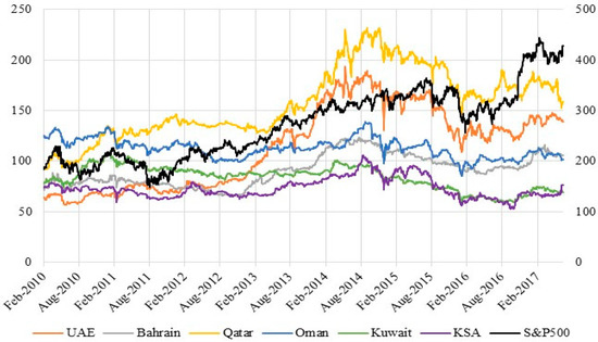
Figure 1.
Time series plots for daily GCC and S&P 500 banking sector price indices for the period February 2010 to June 2017 (S&P 500 banking sector prices indicated on the right axis).
Figure 1 shows three subperiods related to the movement of bank stock prices. The first subperiod (2010–2012) was characterized by relatively stable prices. This period was strongly influenced by post-GFC turbulence and tentative recovery. In considering this context, it should be noted that the GFC itself originated in the US banking sector. During the second subperiod (2012 to mid-2014), bank stock prices showed a steep upward trend. The third subperiod was characterized by a decreasing trend, with a distinct trough in late 2015. This situation was mainly caused by a sharp fall in oil prices. Indeed, the Arab Gulf countries are highly vulnerable to oil price shocks because of their complete dependence on oil export revenue. Table 1 shows the basic statistics for the daily return series.

Table 1.
Stochastic properties of the banking sector return and the unconditional correlation matrix.
Table 1 shows that the US and GCC banking sectors yielded considerable risk−return differences, with the closest coupling attributed to US banks. There were also significant differences between the paired mean risk−returns among GCC bank sectors. In fact, the lowest risk was attributed to Oman and Kuwait, whereas the highest was realized by UAE banks. Saudi banks were well positioned with regard to achieving moderate mean risk-returns over the period.
The skewness values showed a fat tail on the left of the return’s distribution for the banking indices of the US, Bahrain, Kuwait and Oman. UAE, Qatar and Saudi Arabia did not share this feature because their skewness was positive. Further, all our time series had leptokurtic shapes arising from higher excess kurtosis. This higher peak suggested that the times-series distributions were non-normal, which essentially meant that extreme events occurred more frequently over our sample periods. Under the null hypothesis of a Gaussian distribution, the Jarque−Bera statistic rejected the null hypothesis of all series at the 5% significance level. Overall, all index returns did not follow a normal distribution.
The Lagrange multiplier test for autoregressive conditional heteroscedasticity effects and the Ljung−Box test confirmed the presence of a significant conditional heteroscedasticity and serial correlations in the data, which justified the application of the more complex GARCH family of models to the data. Additionally, the results of the two unit root tests (i.e., augmented Dickey−Fuller and Phillips−Perron tests) and the Kwiatkowski−Phillips−Schmidt−Shin test of stationarity showed that the examined return series were stationary.
To initially explore the dependence pattern in our dataset, we first used the Pearson correlation coefficient, as shown at the bottom of Table 1. It was apparent that all correlations between the US and the six GCC banking sectors were significantly close to zero. Among the GCC banking stock market indices, UAE and Qatar had the highest codependence levels. Excluding this relationship, the other participants had positive but relatively weak correlations with each other, signifying the presence of a certain degree of heterogeneity between GCC participants in terms of their banking system structures (i.e., conventional banks, Islamic banks, Islamic branches/windows of conventional banks, etc.).
These differences between GCC participants motivated us to study each country individually instead of the group as a whole. In contrast, it is known that the strength of the relationships between assets varies over time. In addition, numerous studies have shown that financial asset returns tend to be more closely correlated during downside market movements than during upside market movements see, e.g., Ref. [24]. Consequently, our analysis was subsequently focused on dependence models with static and time-varying parameters, specifically considering upturn and downturn stock market conditions.
3.2. Methods
3.2.1. Marginal Model Estimates
To construct the VaR-CoVaR method using copulas, we first needed to specify the marginal distribution for the single series. Among the immense number of GARCH models, we proposed a combined autoregressive moving average (ARMA) model with a Glosten−Jagannathan−Runkle (GJR)-GARCH model and assumed that innovations follow a skewed t-distribution rather than a Gaussian distribution to better account for the existence of heteroscedasticity, asymmetry and leverage effects.
We started by specifying the best ARMA model for each individual stock return series before fitting GJR-GARCH models to their residuals. This is formulated for each return series , where , as:
where and are the autoregressive and moving average parameters with u and v orders, respectively. The GJR-GARCH model is expressed as:
where parameter captures the leverage term, and I is an indicator function that takes a value of 1 for and 0 otherwise. The parameters have the same restrictions as those of the GARCH model, with the addition of Note that the selection of p, q, u and v of each return series is based on the minimum Akaike information criterion (AIC) for more details see [27].
3.2.2. Tail Dependence Using the Copula Approach
In this paper, we combine copula theory with VaR-CoVaR measures to investigate upside and downside risk spillover and the general dependence structure between the US and GCC banking sectors. We now present a brief overview of basic copula theory. For a complete review of copulas and their fundamental properties, see, for example, Ref. [28].
According to Skalar’s theorem, given two random variables (x1, x2) with marginal distribution F1 and F2 and joint distribution H, there exists a unique copula , such that:
Given that F1 and F2 are absolutely continuous, we can then rephrase Equation (4) as:
where and are uniformly distributed across [0,1], and and are the generalised inverse distribution functions of marginal F1 and F2, respectively. The inversion method may be used to obtain the copulas by replacing the joint density function with marginal probability functions. This replacement is essential for analyzing tail or extreme dependence.
The concept of tail dependence describes the dependence in the extreme parts of the bivariate distribution. It allows us to evaluate the tendency of markets to crash or boom simultaneously [28,29,30] formally define the upper and lower tail dependence coefficients as follows:
where . For there is no tail dependence.
There are numerous different copula functions, five of which are used in this study: elliptical Gaussian and Student’s t copulas and asymmetric (Archimedean) Gumbel, rotated Gumbel and symmetrized Joe-Clayton copulas. The elliptical copulas allow us to analyze potential symmetric tail dependence, while the Archimedean copulas allow us to analyze the asymmetry of upper and lower tail dependence coefficients. This is especially relevant for the computation of CoVaR.
Besides the static modelling of all the above copula functions, we also focus on dynamic dependence by allowing the copula parameters to be time varying according to an evolution equation. Let be the linear dependence parameter of the Gaussian and Student’s t copulas, evolving in ARMA (1, q) fashion as follows [31]:
where is a constant, is an autoregressive term and is the average product over the last q observations of the transformed variables. is the modified logistic transformation to retain the value in the range (−1, 1). By replacing the expression with the expression , Equation (8) can be used for the dynamic Student’s t-distribution. For dynamic (rotated) Gumbel copulas, we use the following ARMA (1, q) process:
Finally, we apply Equations (9) and (10) to express the dynamic tail dependence parameters of the symmetrized Joe-Clayton copula:
where denotes the logical transformation.
3.3. Systemic Risk Measure
As defined by [20], the downside VaR computes the risk of index i at the qth quantile:
where denotes the daily return of index i at time t. is typically a negative number, which can be defined by the marginal models as , where and are the conditional mean and standard deviation computed using Equations (1) and (2), and is designed to capture the qth quantile of the data from the skewed t-distribution.
Likewise, upside VaR computes the risk of index i at the (1 − q) quantile as follows:
In this study, indicates the return of an individual GCC banking sector index, and indicates the return of the Standard & Poor (S&P) 500 banking sector index. The CoVaR for an individual GCC banking sector index i at a level of significance (1 − q) can be formally expressed for a specific time horizon with respect to the S&P 500 banking index j being in a state of distress or as its value [20,22] as follows:
Given that Pr ( , CoVaR in Equation (13) can then be shown as:
likewise, the upside for extreme upward return movements in index j or in its value can be formally expressed for a specific time horizon as:
To compute downside and upside using copulas, Equations (13) and (14), respectively, can be used with regard to the joint distribution functions, defined as:
According to [30] theorem, the joint density of two continuous random variables can be described as a function of the copula function. Hence, Equations (15) and (16) can be rephrased as:
Following [21], CoVaR can be calculated from Equations (17) and (18) using the copula function in two steps. First, through the selected copula specifications and for the given values of p, q and , one can solve Equations (17) and (18) to determine the value of . Second, taking , we can assess the CoVaR of x1 with a cumulative probability equal to by inversing F1: . Hence, the copula-based CoVaR needs information only from the cumulative distribution function of the VaR rather than from the VaR itself.
4. Discussion
4.1. Marginal Model Estimates
All parameter estimates of marginal distribution functions are reported by Table 2, which also summarizes the suitable model for the marginal distributions of the S&P 500 and GCC banking sector series. For instance, for the marginal distributions of Kuwait and KSA, we used ARMA (0,0)–GJR (1,1) and ARMA (2,0)–GJR (1,1), respectively. For the mean and variance parameters, we manipulated different parameter combinations. The minimum AIC value was used as the model selection criterion. Moreover, only one lag was used to filter the time series (to eliminate serial dependence).
Table 2.
Marginal model estimates of the ARMA-GJR (1,1) with skew-t distribution.
For the mean equation, all parameters were significant at the 1% level, except for Kuwait and KSA. Note that this bad estimation could bias our subsequent results. For the volatility equation, most parameters were significant at the 1% or 5% levels. In addition, one can see that the parameters (except for the Bahrain banking sector index) suggested a high degree persistence and slow decay of conditional volatility shocks. Moreover, the significant parameter implied that levered effects were found in the sample data (except for the Bahrain series), which was consistent with the sample sign bias test for the series.
The use of asymmetric tail models appeared to be justified, with all coefficients being significant. According to the diagnostic tests (see the bottom of Table 2), the Ljung−Box test statistics were all nonsignificant. Thus, all models appeared adequate to characterize dynamic first and second moments. All p-values related to standard Cramer−von Mises, Kolmogorov−Smirnov and Anderson−Darling (except Bahrain) tests rejected the null hypothesis, confirming that the models were correctly specified.
4.2. Best-Fit Copula
Table 3 reports the estimated time-invariant (Panel A) and time-varying (Panel B) parameters for the copula between the S&P 500 Banking Index and the GCC banking sector indices. From Panel A, the use of AIC allowed us to select the rotated Gumbel copula as the best-fitting model for describing the extreme relationship between the US and banking sectors of four GCC countries, namely UAE, Bahrain, Qatar and Oman. Although the parameters of the rotated Gumbel copulas captured the weak dependence structure of the pairs, they were significant. In contrast, a of 1.048 indicated a persistence in the correlation between the US and UAE banking sectors. Note that the estimated coefficients for Bahrain, Oman and Qatar were close to that of UAE, meaning that all these copulas indicated a strong persistent correlation for tail dependence.
Table 3.
Parameter estimates for the copula between the GCC and S&P 500 banking sector markets.
For the US−Kuwait and US−KSA pairs, the Student’s t and Gaussian copulas had the smallest AIC. For Kuwait, the selected copula also reflected a significant persistence in the estimation of correlation coefficients, with the estimated equal to 1.045. It was also possible that there was no persistence of features in the estimate of the correlation coefficient between the US and KSA because estimated was close to zero.
Panel B shows that, according to AIC, the dynamic rotated Gumbel copula was more appropriate to measure the dependent time dynamics between the US and GCC banking sectors. Moreover, the performance of these dynamic copulas exceeded that of the time-invariant rotated Gumbel copula based on AIC. In fact, for the invariant copula, one might be interested in such measures as rank autocorrelation.
The rotated Gumbel copula had significant lower tail dependence and zero upper tail dependence. One important event pertinent to the selection of this model was that the GFC was characterized by an immense bank failure in the US in 2008 and contemporaneously in many other countries; therefore, there was an implicit contagion effect from US banks to GCC banks. These results may have serious implications for risk management. For instance, the presence of lower tail dependence reflects a much higher risk than in the case of no tail dependence. Further, the range of tail dependence is important to risk-averse investors, who avoid high risk and prefer conservative investments [32].
4.3. Downside and Upside Risk Spillover
Following the results of the best copula model and the two-step procedure described above, we estimated the upside and downside CoVaR at the 95% confidence level (p = 0.05) for the GCC banking sector indices, conditional on the VaR of the US banking sector index at the 95% confidence level (p = 0.05). Figure 2 shows a comparison between the VaR and CoVaR results.
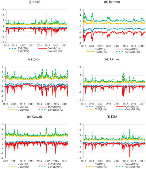
Figure 2.
Downside and upside price spillovers from S&P 500 banking sector to the GCC banking sector markets: (a) UAE; (b) Bahrain; (c) Qatar; (d) Oman; (e) Kuwait; (f) KSA.
It can be seen that VaR and CoVaR measures may vary over time. In addition, there was an asymmetric dependence structure, with a greater lower tail than upper tail dependence. More precisely, we found that both risk measures differed in that downside CoVaRs fell more abruptly than downside VaRs, while upside CoVaRs were closer to upside VaRs, implying that the US banking sector had an asymmetric impact on GCC banking sectors. This also meant that the US and GCC banking indices tended to be more dependent when their returns dropped (i.e., bearish market conditions) than when they appreciated (bullish market conditions). This graphical evidence of the comovement between left tails was in line with our time-varying copula results from the rotated Gumbel copula.
Over the whole sample period, the CoVaR dynamics indicated that the dependence structure changed drastically at the onset of the European debt crisis (from the end of 2010 to the beginning of 2011) and during the mid-2014 oil crisis. During these periods, CoVaR plummeted in value, reflecting an increased systemic risk among the studied countries. Comparing VaR and CoVaR risk measures, we detected the presence of the same systemic risk trend for all countries, but with smaller differences for larger countries. This was consistent with the presence of spillover effects between the banks in US and GCC countries during crisis periods.
These results are partly in line with [23], who found a strong bidirectional return spillover between US and GCC conventional banks. Concerning the high level of resilience detected by Islamic banks, it was important to note that our study cannot accept or reject this conclusion because our results were based on S&P 500 indices determined by banks trading between GCC countries. In addition, even though GCC banks are dominated by domestic and traditional banks, we find that they are sensitive to the losses of US banks. They depend not only on the relationship between both financial channels but are also vulnerable to the behaviors of investors in the region who use indicators of US economic conditions (bad information) to adjust their views.
4.4. Conditional Diversification Analysis
As presented in Table 1, the results for the unconditional correlation coefficients showed that the GCC banking sector index returns were low but positive in relation to the S&P 500 Banks Index returns. Given these findings, it is apparent that investors in the US can achieve diversified portfolios with GCC banking sector indices.
According to [33], the DCC model can be used to model time-varying dependence. The present study adopted the [34] DCC model using GJR-GARCH to deal with heteroscedasticity effects.
Figure 3 displays the DCC results for the Student’s t copula, indicating that the relationship computed in the overall sample was weak, with mixed signs for most GCC countries, particularly the Kuwaiti banking sector. The only exception was the positive and moderate DCC observed for the KSA banking sector index. Hence, our findings based on unconditional correlations and DCC support the diversification possibilities between US and most GCC banking sectors.
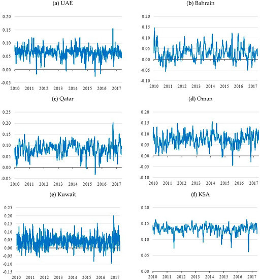
Figure 3.
Time-varying correlations of GCC with S&P 500 for the student-t copula: (a) UAE; (b) Bahrain; (c) Qatar; (d) Oman; (e) Kuwait; (f) KSA.
In line with [35,36], we assessed diversification benefits for portfolios composed of the S&P 500 and GCC banking sector stock markets using conditional diversification benefits (CDB). At time t, the CDB of a portfolio (P) is defined according to the expected shortfall (ES) at level as:
where is the weight of the GCC banking sector indices at time t, and is the q% VaR measure of the portfolio returns. This measure can take values over the interval [0,1]. is the upper bound of the expected shortfall . For = i,j, with as the inverse density function, the expression of the expected shortfall is as follows:
Given that diversification benefits may vary because of readjustments, we evaluate the CDBs of different portfolio compositions for q values of 50% and 5%, which are related to the middle and left extreme values of data distribution, respectively. In this case, we assume that investors want to hold portfolios with unchanged weights over time. Given our Student’s t assumption, the expected shortfall can be formulated using:
where and K denote the cumulative distribution and the standard Student’s t density functions with degrees of freedom, respectively. VaR is specified by:
Figure 4 depicts a time series plot for the CDB of an equally weighted portfolio. We show that diversification benefits are less stable over time and are higher at the 5th percentile than at the 50th percentile of the distribution. More precisely, Figure 4 suggests that CDBs evolve over time, following a path that oscillates around the constant values estimated at the 5% and 50% of data distribution (i.e., 0.65 and 0.25, respectively) along the sample. In other words, our evidence shows that over time, GCC banking sector indices have substantial diversification benefits on US banking stocks, particularly in the 5% extreme left side of the distribution.
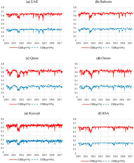
Figure 4.
Time series plot of the conditional diversification benefits of GCCs for S&P 500 banking sector for equally-weighted portfolios: (a) UAE; (b) Bahrain; (c) Qatar; (d) Oman; (e) Kuwait; (f) KSA.
Table 4 shows the CDB for portfolios included in the S&P 500 and GCC banking sector stock markets, as shown in columns 2–6. The first column includes only the portfolio weights for the S&P 500 banking sector. We calculate the diversification benefits of seeing expected shortfall values at 5% (Panel A) and 50% (Panel B) levels.
Table 4.
Diversification benefits of GCCs for different portfolio compositions and probabilities.
The results corroborate the graphical evidence (Figure 4). It can be seen that 5% portfolios have a greater average CDB than do 50% portfolios. Precisely, the CDB of 50% portfolios is negligible, with average values close to zero. Hence, diversification adds no particular value to investor portfolios because it basically involves substitution. However, 5% portfolios increase in size with the weight of US banks in the portfolio. This increase of benefits is concave in shape. Overall, our empirical evidence confirms that a portfolio incorporating US and GCC bank stocks can offer diversification benefits (or a risk reduction) for investors.
5. Conclusions
This paper examines tail risk spillover effects from the US banking sector to the GCC banking sectors, paying special attention to upside and downside stock market conditions. Understanding these tail relationships and risk spillover effects can help fund managers and investors create sound portfolios and make effective asset-allocation decisions when formulating trading and hedging strategies.
We find that the time-varying rotated Gumbel copula is a suitable candidate for effectively modelling this dependence structure. Further, GCC banking sectors receive substantial spillover effects from the US banking sector during downside market movements. Specifically, we find that both risk measures vary in that downside CoVaRs abruptly fell more than downside VaRs, while upside CoVaRs are closer to upside VaRs for all markets (over the period under consideration), indicating that the US banking sector has an asymmetric effect on GCC banking sectors. The results of CDB analysis show significant diversification possibilities for both US and GCC investors.
These findings have at least two important implications for portfolio diversification and hedging decisions. First, the presence of lower tail dependence between US and GCC banking sectors should be considered important by investors and policymakers because both markets could simultaneously crash during crisis periods. Second, the GCC banking sector offers considerable diversification benefits, which are higher in an equally weighted portfolio of US and GCC banking stocks. There is a high diversification benefit or risk reduction for investors who create a diversified portfolio of US and GCC bank stocks, verified by taking into account the tails of their joint distribution. Policymakers in the GCC should remain observant of the impact of extreme downside movements in the US banking sector on GCC banking sectors and intervene when necessary to ensure financial stability.
The results of this study are limited in a sense that we use sector level indices for spillover and diversification analysis without considering the trading cost. Another limitation of this study is the sample period which spans from 2010 and thus does not include the global financial crisis period. Although, we focus on tail dependence and risk spillover during bearish market states, this does not explicitly deal with the issue of financial crisis. Future research on this topic can utilize the data of exchange traded funds and index futures instead of spot prices. Methodological improvement such as combining wavelets and nonparametric test of causality in quantiles [37] could provide a time frequency based relationship for several quantiles.
Author Contributions
Conceptualization, N.S.; methodology, N.T. and F.A.; software, S.J.H.S.; validation, N.S., N.T. and F.A.; formal analysis, S.J.H.S.; data curation, N.S.; writing—original draft preparation, N.S., N.T. and F.A.; writing—review and editing, N.T., F.A. and S.J.H.S.; supervision, S.J.H.S.; funding acquisition, N.S. All authors have read and agreed to the published version of the manuscript.
Funding
This project was funded by the Deanship of Scientific Research (DSR) at King Abdulaziz University, Jeddah, under grant No. G: 400-245-1440. The authors greatly acknowledge DSR’s technical and financial support.
Conflicts of Interest
The authors declare no conflict of interest.
References
- Balcilar, M.; Gupta, R.; Nguyen, D.K.; Wohar, M.E. Causal effects of the United States and Japan on Pacific-Rim stock markets: Nonparametric quantile causality approach. Appl. Econ. 2018, 5050, 5712–5727. [Google Scholar] [CrossRef]
- Balli, F.; Hajhoj, H.R.; Basher, S.A.; Ghassan, H.B. An analysis of returns and volatility spillovers and their determinants in emerging Asian and Middle Eastern countries. Int. Rev. Econ. Financ. 2015, 39, 311–325. [Google Scholar] [CrossRef]
- Ciner, C.; Gurdgiev, C.; Lucey, B.M. Hedges and safe havens: An examination of stocks, bonds, gold, oil and exchange rates. Int. Rev. Financ. Anal. 2013, 29, 202–211. [Google Scholar] [CrossRef]
- Claus, E.; Lucey, B.M. Equity market integration in the Asia Pacific region: Evidence from discount factors. Res. Int. Bus. Financ. 2012, 2626, 137–163. [Google Scholar] [CrossRef]
- Kim, J.S.; Ryu, D. Return and volatility spillovers and cojump behavior between the US and Korean stock markets. Emerg. Mark. Financ. Trade 2015, 51, S3–S17. [Google Scholar] [CrossRef]
- Lien, D.; Lee, G.; Yang, L.; Zhang, Y. Volatility spillovers among the US and Asian stock markets: A comparison between the periods of Asian currency crisis and subprime credit crisis. N. Am. J. Econ. Financ. 2018, 46, 187–201. [Google Scholar] [CrossRef]
- Badshah, I.; Bekiros, S.; Lucey, B.M.; Uddin, G.S. Asymmetric linkages among the fear index and emerging market volatility indices. Emerg. Mark. Rev. 2018, 37, 17–31. [Google Scholar] [CrossRef]
- Lucey, B.M.; Muckley, C. Robust global stock market interdependencies. Int. Rev. Financ. Anal. 2011, 2020, 215–224. [Google Scholar] [CrossRef]
- Majdoub, J.; Mansour, W. Islamic equity market integration and volatility spillover between emerging and US stock markets. N. Am. J. Econ. Financ. 2014, 29, 452–470. [Google Scholar] [CrossRef]
- Singh, M.; Nejadmalayeri, A.; Lucey, B. Do US macroeconomic surprises influence equity returns? An exploratory analysis of developed economies. Q. Rev. Econ. Financ. 2013, 5353, 476–485. [Google Scholar] [CrossRef]
- Fung, A.K.W.; Lam, K.; Lam, K.M. Do the prices of stock index futures in Asia overreact to U.S. market returns? J. Empir. Financ. 2010, 1717, 428–440. [Google Scholar] [CrossRef]
- Alotaibi, A.R.; Mishra, A.V. Global and regional volatility spillovers to GCC stock markets. Econ. Model. 2015, 45, 38–49. [Google Scholar] [CrossRef]
- Ong, L.L.; Pazarbasioglu, C. Credibility and Crisis Stress Testing. Int. J. Financ. Stud. 2014, 2, 15–81. [Google Scholar] [CrossRef]
- Tsuji, C. Correlation and spillover effects between the US and international banking sectors: New evidence and implications for risk management. Int. Rev. Financ. Anal. 2020, 70, 101392. [Google Scholar] [CrossRef]
- Prasad, A. Monetary Policy Transmission in the GCC Countries; IMF Working Papers 20122012; International Monetary Fund: Washington, DC, USA, 2012. [Google Scholar] [CrossRef]
- Istiak, K.; Alam, M.R. US economic policy uncertainty spillover on the stock markets of the GCC countries. J. Econ. Stud. 2020, 4747, 36–50. [Google Scholar] [CrossRef]
- Simpson, J.L. Were there warning signals from banking sectors for the 2008/2009 global financial crisis? Appl. Financ. Econ. 2009, 20, 45–61. [Google Scholar] [CrossRef]
- Arouri, M.E.H.; Lahiani, A.; Nguyen, D.K. Return and volatility transmission between world oil prices and stock markets of the GCC countries. Econ. Model. 2011, 2828, 1815–1825. [Google Scholar] [CrossRef]
- Wang, Y.; Wu, C.; Yang, L. Oil price shocks and stock market activities: Evidence from oil-importing and oil-exporting countries. J. Comp. Econ. 2013, 4141, 1220–1239. [Google Scholar] [CrossRef]
- Adrian, T.; Brunnermeier, M.K. CoVaR. Am. Econ. Rev. 2016, 106106, 1705–1741. [Google Scholar] [CrossRef]
- Reboredo, J.C.; Ugolini, A. Systemic risk in European sovereign debt markets: A CoVaR-copula approach. J. Int. Money. Financ. 2015, 51, 214–244. [Google Scholar] [CrossRef]
- Girardi, G.; Ergün, A.T. Systemic risk measurement: Multivariate GARCH estimation of CoVaR. J. Bank. Financ. 2013, 3737, 3169–3180. [Google Scholar] [CrossRef]
- Mseddi, S.; Benlagha, N. An Analysis of Spillovers Between Islamic and Conventional Stock Bank Returns: Evidence from the GCC Countries. Mult. Finan. J. 2017, 21, 91–113. [Google Scholar]
- Mensi, W.; Hammoudeh, S.; Shahzad, S.J.H.; Shahbaz, M. Modeling systemic risk and dependence structure between oil and stock markets using a variational mode decomposition-based copula method. J. Bank. Financ. 2017, 75, 258–279. [Google Scholar] [CrossRef]
- Shahzad, S.J.H.; Arreola-Hernandez, J.; Bekiros, S.; Shahbaz, M.; Kayani, G.M. A systemic risk analysis of Islamic equity markets using vine copula and delta CoVaR modeling. J. Int. Financ. Mark. Inst. Money 2018, 56, 104–127. [Google Scholar] [CrossRef]
- Trabelsi, N.; Naifar, N. Are Islamic stock indexes exposed to systemic risk? Multivariate GARCH estimation of CoVaR. Res. Int. Bus. Financ. 2017, 42, 727–744. [Google Scholar] [CrossRef]
- Glosten, L.R.; Jagannathan, R.; Runkle, D.E. On the relation between the expected value and the volatility of the nominal excess return on stocks. J. Financ. 1993, 4848, 1779–1801. [Google Scholar] [CrossRef]
- Joe, H. Multivariate Models and Multivariate Dependence Concepts; Chapman and Hall/CRC: London, UK, 1997. [Google Scholar]
- Sibuya, M. Bivariate extreme statistics, I. Ann. Inst. Stat. Math. 1960, 1111, 195–210. [Google Scholar] [CrossRef]
- Sklar, A. Fonctions de repartition an dimensions et leures marges. Publ. Inst. Statist. Univ. Paris 1959, 8, 229–231. [Google Scholar]
- Patton, A.J. Modelling asymmetric exchange rate dependence. Int. Econ. Rev. 2006, 47, 527–556. [Google Scholar] [CrossRef]
- Chai, J.; Du, J.; Lai, K.K.; Lee, Y.P. A hybrid least square support vector machine model with parameters optimization for stock forecasting. Math. Probl. Eng. 2015, 231394. [Google Scholar] [CrossRef]
- Engle, R. Dynamic conditional correlation: A simple class of multivariate generalized autoregressive conditional heteroskedasticity models. J. Bus. Econ. Stat. 2002, 2020, 339–350. [Google Scholar] [CrossRef]
- Brownlees, C.T.; Engle, R. Volatility, Correlation and Tails for Systemic Risk Measurement. SSRN. 2012, p. 1611229. Available online: https://creates.au.dk/fileadmin/site_files/filer_oekonomi/subsites/creates/Seminar_Papers/2012/mes.pdf (accessed on 2 March 2018).
- Christoffersen, P.; Errunza, V.; Jacobs, K.; Langlois, H. Is the potential for international diversification disappearing? A dynamic copula approach. Rev. Financ. Stud. 2012, 2525, 3711–3751. [Google Scholar] [CrossRef]
- Christoffersen, S.E.; Simutin, M. On the demand for high-beta stocks: Evidence from mutual funds. Rev. Financ. Stud. 2017, 3030, 2596–2620. [Google Scholar] [CrossRef]
- Jeong, K.; Härdle, W.K.; Song, S. A consistent nonparametric test for causality in quantile. Economet. Theor. 2012, 2828, 861–887. [Google Scholar] [CrossRef]
Publisher’s Note: MDPI stays neutral with regard to jurisdictional claims in published maps and institutional affiliations. |
© 2020 by the authors. Licensee MDPI, Basel, Switzerland. This article is an open access article distributed under the terms and conditions of the Creative Commons Attribution (CC BY) license (http://creativecommons.org/licenses/by/4.0/).