Abstract
A second-order sliding mode (SOSM)-based direct power control (DPC) of a doubly-fed induction generator (DFIG) is introduced in this research paper. Firstly, the DFIG output powers are regulated with the developed SOSM controller-based DPC scheme. The Super Twisting Algorithm (STA) has been used to reduce the chattering phenomenon. The proposed strategy is a combination of the Lyapunov theory and metaheuristics algorithms, which has been considered to identify the optimal gains of the STA-SOSM controllers. The Lyapunov function method is employed to define the stability regions of the controller parameters. On the other hand, the metaheuristics algorithms are mainly employed to select the fine controllers’ parameters from the predefined ranges. A Thermal Exchange Optimization (TEO) method is used to compute the optimal gain parameters. To prove the superiority of the proposed TEO, its obtained results have been compared with those obtained by other algorithms, including particle swarm optimization, genetic algorithm, water cycle algorithm, grasshopper optimization algorithm and harmony search algorithm. Moreover, the results of the introduced TEO-based SOSM controller have been also compared with the Proportional-Integral (PI)-based vector control and the conventional sliding mode control-based DPC. Moreover, an empirical comparison is carried out to investigate the indication of every metaheuristics method by employing Friedman’s rank and Bonferroni tests. The main findings indicate the effectiveness of STA-SOSM control for system stability and power quality improvement. The ripples in the active and reactive powers are minimized and the harmonics’ distortions of stator and rotor currents are improved. Besides, the STA-SOSM controller shows a superior performance of control in terms of chattering phenomenon elimination.
1. Introduction
In recent years, the utilization of renewable energy sources has prompted a reduction in conventional fossil-fuel energy source dependency. Wind energy as a renewable source has gained considerable attention because it is clean and pollution-free. It has undoubtedly been the most growing source in terms of installed capacity. Wind Energy Conversion Systems (WECSs) are mainly based on wind turbines (WTs) that convert kinetic energy to electrical energy through an electrical generator. However, the intensive studies that have been carried out in the wind technology market produced different wind energy configurations. The most popular configuration is the Doubly-Fed Induction Generator (DFIG) linked with the WTs. This type is vastly used due to its considerable advantages, of which the decoupled control of active and reactive powers, low converter costs and mechanical exertion decrease are the main ones. The DFIG is basically a wound rotor generator. The rotor windings are linked to the utility grid via a power converter consisting of a Rotor-Side Converter (RSC) and a Grid-Side Converter (GSC). This topology enables the converter to catch the portion of 20% to 30% of the overall power, resulting in reducing its cost. As such, losses in the converter are less resulting in an amelioration in the overall performance. However, according to the Global Wind Energy Council’s report of 2018, DFIG-based wind converter systems are approximately 243.4 GW of the overall 568.409 GW wind power investiture. This means that DFIG occupies close to 50% of total wind power generation [1].
Several research works have assured reinforcement of the efficiency of WECSs. It is well established that the DFIG running under variable wind speeds to allow capturing the maximum amount of wind power. To achieve this goal, there exist various control strategies. The classical Vector Control (VC) scheme is broadly applied for both RSC and GSC converters. This scheme allows independent control of the power components exchanging between the DFIG and the grid, keeps the Direct Current (DC)-link voltage constant and realizes the maximum power point tracking. The VC method is mostly attained by regulating the decoupled rotor converter currents using linear Proportional-Integral (PI) controllers [2]. The major disadvantage of this scheme is that the effectiveness of the DFIG system substantially relies on the accurate adjusting of the PI parameters and the exact values of DFIG parameters, such as stator resistance, rotor resistance and inductances. Hence, the PI controllers-based VC method provides poor performance and low robustness, especially when actual DFIG parameters deviate from the nominal values which have been used in the control system [3,4,5].
In this regard, to overcome the shortcomings of the VC method based on linear controllers, a number of the non-linear control strategies have been proposed in the literature. In [6], Direct Power Control (DPC) is perfectly performed using the fuzzy logic control strategy. Stator power components are regulated and contrasted with the linear PI type. In [7], a hybrid control based on a PI controller combined with fuzzy logic is adopted to perform the DPC strategy. Although the results from the fuzzy-based controller introduced better performance over PI-based controller, the difficulty in fuzzy logic was in the determination of suitable fuzzy rules. A model-based predictive DPC method was achieved in [8]. The stator power components were predicted in one period of the sampling frequency, in which the rotor voltage was calculated based on this prediction. The predictive control strategy introduced a better solution but it was prone to computational problems. In [9], a hybrid controller based on the multivariable generalized predictive control model and the H∞ controller was implemented. The predictive control term ensured the convergence feature while the H∞ control strategy was adopted to reinforce robustness under external disturbances. DPC regulation was proposed using the Artificial Neural Network (ANN)-based system. The proposed ANN system adopted an individual training technique using fixed-weight and supervised models. This led to a lower execution time and, therefore, the errors caused by control time delays were reduced. Although the ANN-based controller presented better performance over the linear PI controller, there were some problems in the execution of the ANN [10].
Apart from the aforementioned approaches, the Sliding Mode Control (SMC) based technique has recently been proposed for the DFIG-based WECS. The strengths of SMC lie in its robust nature performance against uncertainties, parametric mismatch, external unknown disturbances, fault conditions, fast convergence and simplicity to implement. Indeed, the majority of WTs are established in rural regions and linked to prosaic grids where dense unsymmetrical loads and voltage dips happen frequently. Therefore, a robust control approach should be used to ensure the performance of the DFIG-based WECS and the SMC-based approach is the most suitable candidate. In [11], the classical SMC has been adopted to perform the DPC strategy at the stator side by applying the PI controller to the DC-link voltage. The sliding surface was selected according to the tracking error and its integration. In [12], the conventional SMC is applied to regulate the rotor speed and the DC-link voltage. However, the chattering problem remains the most serious challenge when implementing the SMC strategy, which may involve high control activity and excite unmodeled dynamics. Several methods were applied to outperform the issue. In [13], the fast exponential reaching law-based SMC was carried out and compared with the classical exponential reaching law. In [5], a new SMC law was developed to perform indirect power control, of which the tracking performance and the robustness to uncertainties were enhanced. In these studies, the chattering phenomenon was clearly reduced. However, an efficient approach to outperform the chattering issue is to employ high-order sliding mode ones. In [14,15], the Super Twisting Algorithm (STA)-based Second-Order Sliding Mode (SOSM) controller is applied to perform DPC regulation, which introduced better performance compared to other variants of SMC strategies. However, the question that should be highlighted is related to the selection of the optimal STA-SOSM controllers’ gains. Although these gains are positive, tuning these effective design parameters to obtain high control performance is a very hard task. Moreover, the majority of the SMC parameters are adjusted with the manual trial-and-error method, which remains difficult and time-consuming. Therefore, introducing a methodical approach to attain the fine gains setting of STA-SOSM controllers is a challenging activity. To this end, metaheuristic optimization algorithms are recently nominated as an appropriate solution.
In this context, several methods have been applied to select the gains of SMC controllers. In [16], the Fractional-Order Sliding Mode Controller (FOSMC) is introduced to control the stator power components of DFIG. The multi-objective grey wolf optimizer was applied to adjust the parameters of FOSMC. In [17], the DPC strategy is performed by using STA-SOSM control and the Lyapunov theory was applied to determine the ranges of controllers’ gains. In [14], the DPC approach is also implemented, in which tuning equations are derived to adjust the gains of the STA-SOSM controllers. In [18], the direct torque control of the DFIG using the STA-SOSM strategy was implemented. The rooted-tree optimization algorithm was used to search the optimal gains of the STA-SOSM controllers. Ripples in the torque and rotor speed were decreased while the system rapidity increased.
In this paper, the STA-SOSM control strategy is proposed to achieve the direct power control of the DFIG and keep the DC-link voltage at the GSC constant. The main contribution of this work is to provide a combination method of the Lyapunov theory and metaheuristics algorithms to find the optimal gains of STA-SOSM controllers. The Lyapunov theory is adopted to define the ranges of controllers’ parameters to ensure the system’s stability, whereas metaheuristics algorithms are mainly employed to select the fine controllers’ parameters from the predefined ranges. The main contributions of the proposed designed controller are that it (1) increases the robustness and stability of the controlled system; (2) provides methodical and less-complicated proceedings based on a novel TEO method to adjust the gains of the controllers; (3) minimizes ripples in the active and reactive powers; (4) improves the Total Harmonic Distortion (THD) of the stator and rotor currents. The well-known metaheuristics algorithms are Particle Swarm Optimization (PSO), Genetic Algorithm (GA), Water Cycle Algorithm (WCA), Grasshopper Optimization Algorithm (GOA), Harmony Search Algorithm (HSA) and Thermal Exchange Optimization (TEO). An empirical comparison study between the metaheuristics algorithms is achieved. Besides, statistical tests are carried out to assess the significance of each method. Furthermore, the performance of the STA-SOSM control strategy is compared with linear PI controllers for reference tracking, parameter variations and voltage dip conditions.
This paper is arranged as follows: Section 2 explains the mathematical representation of the DFIG model. Section 3 shows the representation of the applied super twisting algorithm-based second-order sliding mode on the DFIG system. Besides, the same section specifies the formularization of the STA-SOSM controller’s adjusting issue that will be resolved by the recent metaheuristics algorithms. Section 4 presents the implementation and the validation of the proposed metaheuristics algorithms with the Lyapunov theory for tuning the STA-SOSM controller. Concluding remarks are given in Section 5.
2. Model Statement
2.1. Wind Turbine Model
The WT is in charge of capturing wind energy and transforming it into kinetic energy. The harnessed mechanical power is expressed as [19]:
The power conversion efficiency is a dimensionless coefficient, which is a function of the tip speed ratio and pitch angle. Based on the wind turbine characteristics, the power coefficient can be calculated from the following general expression [7]:
where , , , , , and is defined as:
The tip speed ratio is expressed as a relation between the blade tip speed and the wind speed. It is given by:
If the wind speed is below the rated value, the power coefficient should remain at its maximum value by applying the Maximum Power Point Tracking (MPPT) strategy and deactivating the pitch control. If the wind speed exceeds its rated limit, the pitch mechanism is switched on to decrease the extracted mechanical power.
2.2. Doubly Fed Induction Generator Model
The mathematical representation of the DFIG model can be defined as follows [20]:
In this study, Stator Flux Orientation (SFO) is used to perform the power control of the DFIG. Supposing that the electrical grid is stable, the stator flux is constant. Besides, for high-power DFIGs, the stator resistance can be ignored due to its small value [21]. Therefore, according to the above presumptions, the stator voltages and fluxes can be written as follows [20]:
The stator power components and rotor voltages are expressed as [5,22]:
where and .
2.3. Grid-Side Converter and DC-Link Models
The GSC part is joined to the grid via an Inductance (L) capacitance (C) inductance (L) circuit (LCL)-filter to a better harmonic reduction of the grid currents. The mathematical model of the GSC in the dq frame is expressed as in Equation (10). At the fundamental frequency, an LCL-filter can be approximated to an L-filter [21]:
where is the sum of the converter-side and grid-side resistors, and represents the sum of the converter-side and grid-side inductances.
The DC-link circuit, which connects the GSC and RSC components, can be modeled as follows [5,12]:
where is the current flowing between the DFIG rotor and the DC-link. From the voltage dynamics given by Equation (11), the DC-link voltage can be controlled via the direct grid current.
3. Metaheuristics-Based Integral Sliding Mode Control Strategy
3.1. Problem Statement
The main objective for controlling the RSC circuit is to independently regulate the stator active and reactive powers. The nonlinear Super Twisting Algorithm (STA)-based Second-Order Sliding Mode (SOSM) control scheme is employed to directly calculate the required rotor control voltage without a need to use extra current control loops [11,14]. The proposed STA-based SOSM control scheme is depicted in Figure 1.
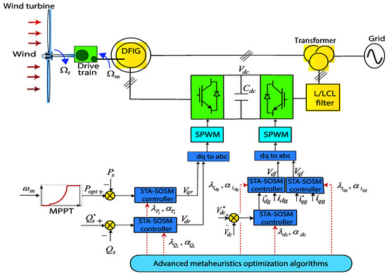
Figure 1.
Metaheuristics-tuned direct power control block diagram of the doubly-fed induction generator (DFIG)-based Wind Energy Conversion System (WECS).
To track the stator power component references, the following sliding surfaces are selected:
where and denote the tracking errors between the set-point values and actual values of the active and reactive stator powers, respectively, and and are positive parameters to be tuned. The integral terms are adopted to reinforce the transient response and minimize the steady-state error [11].
According to Equations (8) and (9), the dynamics of the switching variables given in Equation (12) are expressed as:
where ; ; ; and and , are the perturbation terms related to the unmodeled dynamics, parameters’ uncertainties and any external disturbance at the reactive and active powers loops, respectively [5].
In the DPC of the DFIG system, the stator power components are controlled by regulating parts of the converter voltage at RSC circuit. Therefore, the rotor converter voltages are selected to be the control output variables. From Equations (12) and (13), it can be deduced that:
It can be noted that the relative degree concerning is a first-order relative degree. Similarly, the relative degree with respect to equals 1 as well. Consequently, the DPC scheme may be achieved by applying classical SMC or STA-SOSM approaches. Thus, the voltages to be forced to the rotor circuits components based on STA-SOSM controllers can be calculated as follows [19,23]:
The last control laws contain the equivalent and super twisting terms. The main objective for super twisting terms is to ensure that the switching surfaces and are attained in a finite time. Furthermore, the equivalent control terms and aim to make the system slide the sliding manifold. However, the equivalent control terms can be directly calculated by forcing .
The proposed and voltages are defined as follows [24,25,26]:
where , , and are positive control parameters to be designed, is the mathematical sign function and , are the integral actions of the super twisting terms for the power control law components. From Equations (15) and (16), it can be deduced that the control laws applied to the rotor voltage dynamics are given by:
Finally, the proposed DPC strategy based on the STA-SOSM approach, which is designed for active and reactive power regulation of the DFIG, is shown in Figure 2.
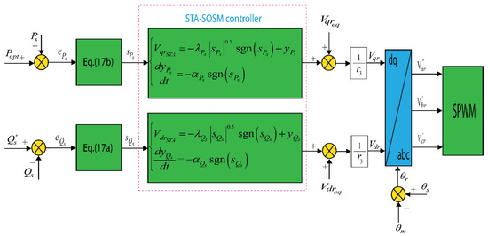
Figure 2.
Block diagram of the rotor-side converter (RSC) with the proposed direct power control (DPC) strategy based on super twisting algorithm-based second-order sliding mode (STA-SOSM) controller.
Moreover, to make the DC-link voltage constant, the direct grid current is regulated thanks to a designed STA-based SOSM controller. The quadrature one can be utilized to control the reactive power exchange between the GSC and the grid [27].
The DC-link voltage dynamics (11) can be rearranged under the following form [12]:
where and denotes the perturbation term at the DC-link voltage loop.
Let us define the dynamics of the DC-link voltage error as follows [22]:
The time derivative of the sliding surface is as given:
where is the new control input.
Finally, the control input is given as:
where and are positive control parameters to be designed, is the mathematical sign function, is the integral action of the super twisting term for the DC-link voltage control law and .
In high dimensional systems, the choice of the control parameters of the SOSM is a big challenge, where optimal gain parameters ensure the stability and robustness of the system and introduce a fast response. Control parameter adjustment with the classical manual trial-and-error method is a time-consuming procedure. Furthermore, the selection of SOSM coefficients based on other methods, such as Hurwitz stability analysis and linearization around the equilibrium point, can achieve stability of the control law but without ensuring that the obtained parameters are the optimal ones. To alleviate the selection of the control parameters of the SOSM control the thermal exchange optimization algorithm will be adopted to solve the tuning issue, in which the limitations of the control parameters are used as inequality constraints for the optimization problem. This leads to an increase in the tracking performance a system and eliminates the chattering problem.
3.2. Robustness and Operational Constraints
Lyapunov stability analysis of the DFIG-based wind converter dynamics leads to nonlinear constraints on the decision variables of the formulated control problem. The stator reactive power loop is considered for this analysis since the same methodology can be applied to the stator active one. By using the control law (17) and taking into account the time derivative of the slide surface as given in Equation (13), the dynamics of can be represented as follows [23,25]:
Let us consider that the perturbation term of the system (13) is globally bounded as follows:
where is a positive constant.
Now, the following quadratic Lyapunov function is selected as a candidate function as follows:
where and is a positive definite matrix with the following form:
The first time derivative of can be expressed as follows [17]:
where and .
Then, the time derivative of along the trajectories of the system (16) is computed as:
where and .
Using the bounds on the perturbation (23), it can be demonstrated that [25]:
where the matrix is expressed as:
when this matrix is symmetric and positive definite, i.e., , there exists a candidate Lyapunov function (24) satisfying and the control system will reach to the origin in a finite time. So, to have as a positive definite matrix, the range values of and should respect the following nonlinear constraints:
To have the stability condition related to the sliding variable , the same methodology is adopted as for the stator reactive one. Similarly, the range values of and are derived as follows:
For the DC-link voltage dynamics, the limitations of the effective control parameters are determined as:
where is a positive constant.
Moreover, the stability conditions for the parameters of the grid current controllers are:
where can represent the d or q axis. For some constants .
3.3. Control Problem Formulation
Although the convergence of the sliding surfaces can be guaranteed, an important question should be highlighted. This question is related to the selection of the optimal STA-SOSM controller’s gains. Although we know that the gains and for are positive, tuning these effective design parameters to obtain a high control performance for the studied DFIG system is a very hard task. Poor tuning of the gains may lead to deteriorating the system control performance. Moreover, the majority of the SMC parameters are adjusted with the manual trial-and-error method, which remains difficult and takes much time [28].
In this work, five STA-SOSM regulators for the external and inner-loops at the RSC and GSC circuits are taken into account for the optimization procedure. These nonlinear and robust regulators for the stator power component dynamics, DC-link voltage and grid current components are systematically designed and tuned thanks to the proposed TEO algorithm. However, more details about the TEO can be found in [20,29].
The decision variables of the formulated hard optimization problem are obviously the and parameters for the designed STA-SOSM controllers (17) and (21). They are specified for the optimization process as:
where denotes the bounded search space for the STA-SOSM controllers’ tuning problem. For optimal control approaches, the objective functions are defined by popular performance criteria, such as Integral Absolute Error (IAE), Integral Square Error (ISE), Integral Time-weighted Absolute Error (ITAE) and Integral Time-weighted Square Error (ITSE). The targeted cost functions are optimized considering the time-domain constraints, such as the overshoot, steady-state error and rise and/or settling times [21,30]. To enhance the performance of the controller through a proper selection of SOSM parameters, the defined stability and robustness conditions in Equations (30)–(33) are forced as inequality constraints for the formulated optimization problem. Therefore, the adjusting problem associated with the STA-SOSM regulators of the DFIG is completely formulated as a constrained optimization problem as follows:
where are the cost functions, are the problem’s inequality constraints, and are the overshoots of the DC-link voltage, grid current components and stator power components, respectively. The terms and indicate their maximum specified values.
The optimization issue (35) is a multi-objective kind. Therefore, the weighted sum-based aggregation functions are adopted to hold these multiple costs. The objective function is defined using the IAE index as:
where denotes the total simulation time, are the weighting coefficients satisfying and are the tracking errors defined , , , and .
3.4. Thermal Exchange Optimization Algorithm
The thermal exchange optimization (TEO) method is an advanced algorithm devised by Newton’s law of cooling [29]. In the TEO algorithm, every agent is considered as a cooling object. By contacting another object as an enclosure fluid, heat is transmitted and a thermal interchange happens between them. The new temperature of each agent is considered as a new position of the potential solution in the search space.
In the search space, at the iteration, every agent is defined by its temperature , . In order to reinforce the optimization abilities, the TEO method utilizes thermal memory (TM) to save some of the best chronological vectors and its related fitness. So, these saved resolution vectors are supplemented to the population and the same amount of existing worst agents is removed. After that, a growing order of solutions is saved based on its objective function values. The saved agents are evenly parted into two sets of environment and cooling agents. The environment objects are denoted as while the cooling ones are .
Since the agent that has lower can exchange temperature slightly, the proposed method developed a similar equation to estimate the value of for each agent as given in (37):
As the iterations increase, the value rises, resulting in upgrading the exploration technique. To reinforce the TEO method’s exploration ability, Formula (38) is introduced to prevent enclosing in local optima and to renovate the environmental temperature:
where and are the controlling variables chosen as 0 or 1, is a uniformly random number, is the former environmental temperature and is introduced to minimize the randomness by closing to the last iterations. When decreasing of the randomness is not required, the value of is set to zero.
The new temperatures for each object, i.e., either cooling objects or environmental ones, are updated as:
In the TEO method, another equation is introduced to upgrade the exploration mechanism. Control input is adopted and decides whether a term of every cooling agent must be altered or not. For every agent, such an input is contrasted to . If , one term of the agent is selected indiscriminately and its value is renewed as [29]:
where is the term of the object, and are the superior and lower limits of the term, respectively.
The flowchart explains the introduced metaheuristics-based adjusting method of the SOSM regulators in the DFIG system, as shown in Figure 3.
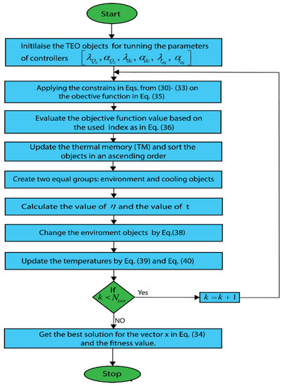
Figure 3.
Flowchart of the proposed thermal exchange optimization (TEO)-tuned SOSM controller parameters.
4. Results and Discussion
This part introduces the simulations performed to investigate the effectiveness of the proposed metaheuristics-based STA-SOSM controllers for the studied DFIG. The main components of the WECS are discussed, with a special focus on the control of electrical magnitudes at the RSC and GSC of DFIG systems, such as active/reactive powers and DC-link voltage. The proposed global metaheuristics-based STA-SOSM controller design was constructed through MATLAB/Simulink. The parameters of the studied DFIG-based WECS are listed in [21].
4.1. Convergence Rates
To investigate the effectiveness of the proposed metaheuristics, the introduced algorithms GA [31], PSO [32], HSA [33], WCA [34] and GOA [35] were executed with the same values for the common parameters, i.e., population size and the maximum number of iterations . To find accurate values of the decision variables , the bounded search domain was set to and is the minimum limit of the decision variables that is determined by Equations (30)–(33).
Table 1 gives the optimization results of the problem (35). The bold and underline values represent the best convergence values for each index. It can be obviously noted that the introduced TEO and GA produce highly competitive solutions with the other methods. Table 2 lists the acquired parameters of the STA-SOSM regulators for each proposed optimization algorithm. In fact, these adjusted STA-SOSM regulators’ parameters result in better transient and steady-state responses of the whole introduced methods. Besides, Figure 4 displays the convergence histories of the mean cost functions for four indices. Moreover, it is clear that the TEO method for the ISE and ITSE indices copes the other introduced algorithms in terms of speed and non-premature convergence. Figure 4a,c state that the TEO-based algorithm for the IAE and ITAE indices displays the better convergence as a second and third-order respectively after the GA one. These results confirm that the superiority of the TEO method is still in terms of exploitation and exploration mechanisms. The Box-and-Whisker plots of the mean objective function values are shown in Figure 5 and further prove the superiority of the proposed TEO-based tuning approach.

Table 1.
Optimization results of the problem (35).
Table 2.
Optimized decision variables of problem (35).
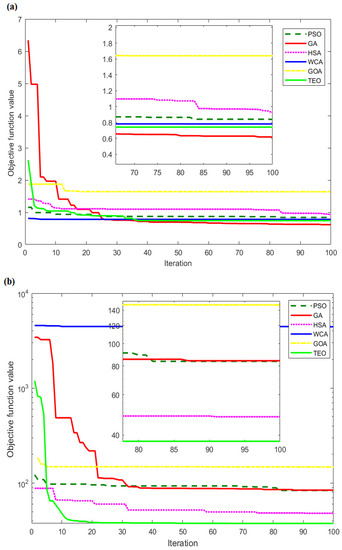
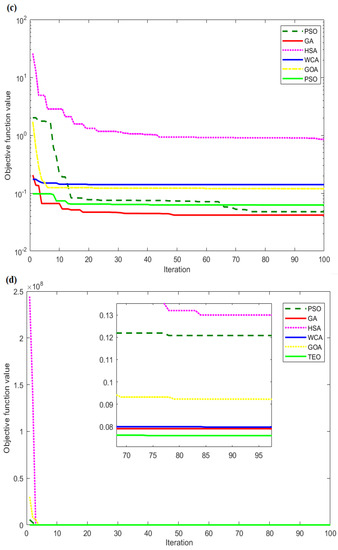
Figure 4.
Convergence histories: (a) Integral Absolute Error (IAE); (b) Integral Square Error (ISE); (c) Integral Time-weighted Absolute Error (ITAE); (d) Integral Time-weighted Square Error (ITSE) index.
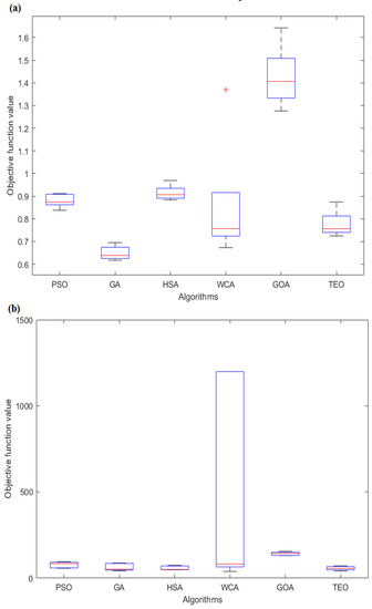
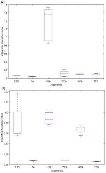
Figure 5.
Box-and-whisker plot: (a) IAE; (b) ISE; (c) ITAE; (d) ITSE index.
4.2. Statistical Analysis and Comparison
4.2.1. Friedman’s Test
The mean values concerning the various optimization indices are classified to evaluate the most optimal one according to its average cost function. Besides, a statistical study based on Friedman and Bonferroni–Dunn’s tests is executed by utilizing these mean values [21]. The average ranks for all the reported algorithms based on the considered criteria are summarized in Table 3. We can obviously observe that the introduced TEO method and GA have the lowest ranks as marked in the bold and underline in comparison with the rest of the algorithms.
Table 3.
Ranking of algorithms based on the statistical study.
Friedman’s test provides the computed value of the -distribution. Since the computed score is greater than the statistical value, the null hypothesis is rejected. Furthermore, by applying the Iman-Davenport test [36], the null hypothesis is also rejected as the calculated value is greater than the critical value at the same significance level. These statistical results denote that there are significant differences between the effectiveness of the presented methods.
4.2.2. Bonferroni–Dunn’s Test
However, a post-hoc Bonferroni-Dunn’s test was applied to test whether or not the presented TEO method is significantly superior to another method [21]. The TEO and GA algorithms have the same performance. Therefore, this test was performed to investigate the differences between the TEO and other algorithms except for GA. The corresponding Critical Differences (CDs) of the reported algorithms at the confidence levels 95% and 90% are computed as and . Figure 6 shows the representation of the Bonferroni–Dunn’s test, taking into account that the TEO is a control method. The GOA and HSA methods violate the horizontal line of 95% significant level. This indicates that the TEO method works at least remarkably better than the GOA and HSA methods at a 95% significance level over the solutions equality [37].
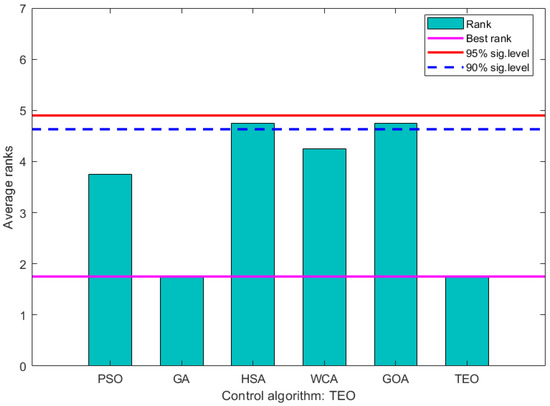
Figure 6.
Graphical representation of the Bonferroni-Dunn’s test for problem (35).
4.2.3. Elapsed Time Efficiency
According to the average elapsed times that were listed in Table 1, the Computational Time Efficiency (CTE) [38] for every method over the presented optimization index is listed in Table 4. In terms of computational time, it can be noted that the introduced TEO method achieved the second-best average elapsed time, whereas the GOA metaheuristic achieved the best average elapsed time.
Table 4.
Measures of algorithms’ CTE metrics for problem (35).
4.3. Reference Tracking Condition
The target of this scenario is to evaluate the behavior of the STA-SOSM and vector control-based PI strategies. The stator reactive power, DC-link voltage and THD of the stator and rotor currents are adopted for making a fair comparison. However, the gains obtained by the TEO algorithm are used. As shown in Figure 7a, for the two control strategies, the stator reactive power perfectly tracks their references values, for which the STA-SOSM controller introduces better performances in terms of overshoot damping, settling time and steady-state error decreasing. However, the PI controller presents a faster time response. It can be noted from Figure 7b that both controllers introduce a good tracking performance with a remarkable superiority of the STA-SOSM controller in terms of rise time, settling time and steady-state error decreasing. To further compare the performances of these two methods, the stator and rotor currents’ harmonic spectra are compared. Figure 8 states that the THD of the stator current is better for the STA-SOSM strategy (THD = 0.28%) when compared to the PI controller one (THD = 0.77%). Furthermore, the THD of the rotor current for the STA-SOSM controller (THD = 0.32%) is less than obtained by the PI one (THD = 0.85%), as stated in Figure 9.
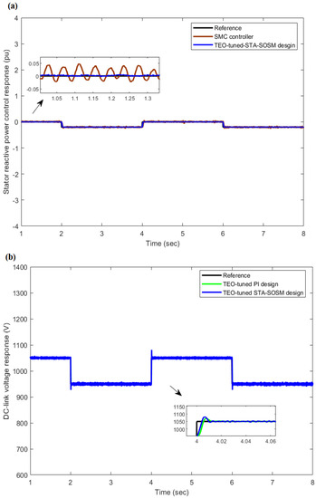
Figure 7.
Performance comparison: (a) stator reactive power; (b) DC-link voltage.
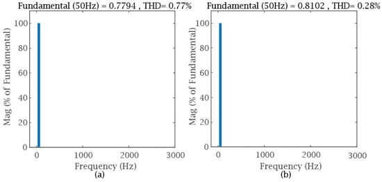
Figure 8.
Stator current harmonic spectra: (a) Proportional-Integral (PI) controller; (b) STA-SOSM controller.
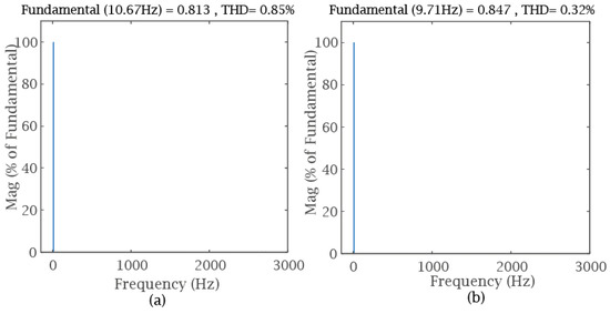
Figure 9.
Rotor current harmonic spectra: (a) PI controller; (b) STA-SOSM controller.
Figure 10a,b show the dynamic performances of the controlled stator reactive power and DC-link voltage against the chattering behavior of the time-domain responses. It is clearly observed that the undesirable phenomena in the stator reactive power and DC-link voltage dynamics are reduced with the proposed TEO-tuned STA-SOSM controller in comparison with the conventional SMC method.
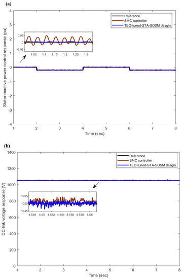
Figure 10.
Chattering attenuation: (a) stator reactive power; (b) DC-link voltage.
4.4. Robustness Analysis
4.4.1. Parametric Mismatch Condition
Further tests of the impact of the DFIGs parameter variations on the dynamics performance of the control strategies will be presented. To this end, the proposed STA-SOSM and vector control-based PI strategies are investigated. Figure 11, Figure 12 and Figure 13 show the simulation results with variations in inductance and resistance values. For this test, the demonstrative figures will present the dynamical performances of the electromagnetic torque and DC-link voltage as well as the stator active and reactive powers for the STA-SOSM and the PI controllers at each scenario. Figure 11 presents the time-domain performances of the aforementioned control loops when the rotor inductance is augmented by 200% of its nominal value.
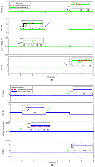
Figure 11.
Simulation results of different control dynamics under the influence of rotor inductance variations: (a) PI controller; (b) STA-SOSM controller.
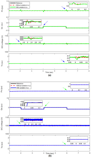
Figure 12.
Simulation results of different control dynamics under the influence of stator inductance variations: (a) PI controller; (b) STA-SOSM controller.
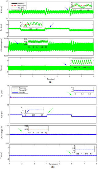
Figure 13.
Simulation results of different control dynamics under the influence of set-of-parameters variations (SPV): (a) PI controller; (b) STA-SOSM controller.
In addition, Figure 12 shows the time domain performances of the control loops in case of the stator inductance variation. Figure 13 shows the time domain performances when more than one parameter are changed. We can clearly deduce that parameter deviations have a clear effect on the dynamic performances of electromagnetic torque, DC-link voltage and stator active/reactive powers when using the PI controller. In addition, the decoupling between the active and reactive powers is not ensured in this case, whereas the proposed TEO-tuned STA-SOSM approach is robust against parameter variations and the decoupling is perfectly ensured.
4.4.2. Grid Faults Condition
DFIGs are very sensitive to grid disturbances because of the direct connection of the stator winding to the grid. In WECSs, dip voltage is not acceptable. Therefore, the performance of the proposed controllers was examined under a dip voltage scenario. The grid voltage dips and the SPV scenarios were tested at the same time. The dynamic responses of the STA-SOSM controlled system and PI are presented in Figure 14, Figure 15 and Figure 16. It can be noted from Figure 14 that the proposed control strategy can successfully mitigate the voltage dip, as the fluctuations in the electromagnetic torque, stator active and reactive powers during the voltage dips were relatively small and the attenuation speed was faster.
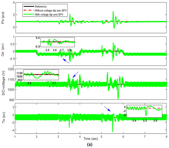
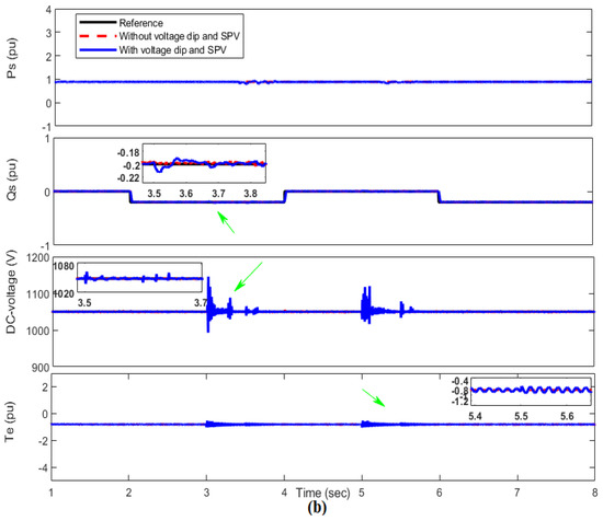
Figure 14.
Simulation results of different control dynamics under unbalanced grid voltage conditions and the influence of SPV: (a) PI controller; (b) STA-SOSM controller.
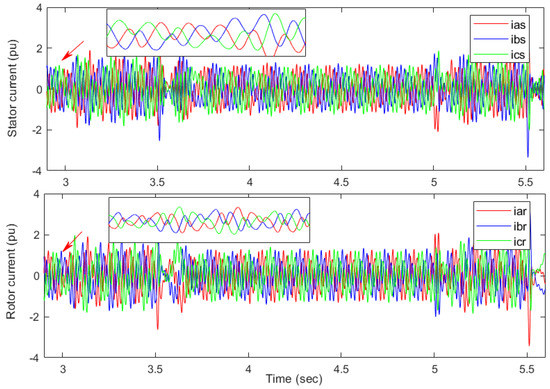
Figure 15.
Simulation results of the stator and rotor currents under unbalanced grid voltage conditions and influence of SPV (PI controller case).
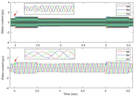
Figure 16.
Simulation results of the stator and rotor currents under unbalanced grid voltage conditions and the influence of SPV (STA-SOSM controller case).
In the PI controller case, there are high amplitude fluctuations in the dynamic responses of the electromagnetic torque, stator active and reactive powers because of the voltage dip condition. However, the proposed STA-SOSM and PI controllers have approximately the same performance in the DC-link voltage response. Moreover, Figure 16 confirms the effectiveness of the proposed STA-SOSM, where the stator and rotor currents are within their predefined ranges. While the stator and rotor currents in case of the PI controller are completely distorted as shown in Figure 15. These results confirm the robustness and ability of the proposed TEO-tuned STA-SOSM controller to deal with voltage dip conditions.
5. Conclusions
This paper discussed and performed a proposed metaheuristics-tuned STA-based SOSM control scheme for the outer- and inner-loops at both RSC and GSC circuits of a DFIG-based WECS. The proposed strategy is a combination of the Lyapunov theory and metaheuristics algorithms, which aims to identify the optimal gains of the STA-SOSM controllers. The Lyapunov theory was used to determine the constraints and limitations of the gains of controllers. The uncertainty model and the external disturbance for stator powers and DC-link voltage dynamics were analyzed and taken into consideration. Then, the tuning issue associated with the STA-SOSM controllers was formulated as a constrained optimization problem, which was solved using the recent TEO algorithm. To investigate the significance of the introduced TEO-based method in attaining the minimum value of the cost function, a comparison study with well-known algorithms was implemented. The simulation results have shown that the introduced TEO-based STA-SOSM controllers have high performances and robustness to uncertainties and parameter mismatches as well as the attenuation of chattering phenomena in comparison with vector control-based PI controllers. The obtained results confirm that the introduced TEO-based algorithm is an appropriate method for regulating the DFIG system by methodically adjusting the unknown STA-SOSM controllers’ parameters effectively.
The current research work is limited by considering that wind speed is fixed. Besides, the proposed method investigated a low voltage dip condition. Stability enhancement of the DFIG system under the previous concerns will be carried out in future work. This will be implemented through interactions among DFIGs with various control methods, such as fractional-order PI and adaptive gain SOSM controllers. Indeed, these methods deserve attention because they solve the difficulty of estimating the uncertainty upper bounds for WECSs.
Author Contributions
Conceptualization, M.M.A., S.B. and H.R.; Data curation, M.M.A.; Funding acquisition, M.M.A.; Investigation, M.M.A., S.B. and H.R.; Methodology, S.B.; Project administration, S.B.; Resources, M.M.A., S.B. and H.R.; Software, M.M.A.; Supervision, S.B. and H.R.; Validation, M.M.A.; Writing—original draft, M.M.A.; Writing—review & editing, S.B. and H.R. All authors have read and agreed to the published version of the manuscript.
Funding
This research received no external funding.
Conflicts of Interest
The authors declare no conflict of interest.
Nomenclature
| DC-link capacitor | |
| Grid voltages in dq reference frame | |
| Grid currents in dq reference frame | |
| Rotor currents in dq reference frame | |
| Stator currents in dq reference frame | |
| Mutual inductance | |
| Rotor and stator inductances | |
| Stator active power | |
| Stator reactive power | |
| Rotor and stator resistances | |
| DC-link voltage | |
| Grid converter voltage in dq reference frame | |
| Rotor converter voltage in dq reference frame | |
| RMS phase voltages for the stator | |
| Stator voltages in dq reference frame | |
| Angular grid frequency | |
| Rotor and stator angular frequencies | |
| Mechanical rotational speed | |
| Rotor fluxes in dq reference frame | |
| Stator fluxes in dq reference frame |
References
- Naik, K.A.; Gupta, C.P.; Fernandez, E. Design and implementation of interval type-2 fuzzy logic-PI based adaptive controller for DFIG based wind energy system. Int. J. Electr. Power Energy Syst. 2020, 115, 105468. [Google Scholar] [CrossRef]
- Pena, R.; Clare, J.; Asher, G. Doubly fed induction generator using back-to-back PWM converters and its application to variable-speed wind-energy generation. IEE Proc. Electr. Power Appl. 1996, 143, 231. [Google Scholar] [CrossRef]
- Poitiers, F.; Bouaouiche, T.; Machmoum, M. Advanced control of a doubly-fed induction generator for wind energy conversion. Electr. Power Syst. Res. 2009, 79, 1085–1096. [Google Scholar] [CrossRef]
- Djoudi, A.; Chekireb, H.; Berkouk, E.M.; Bacha, S. Low-cost sliding mode control of WECS based on DFIG with stability analysis. Turk. J. Electr. Eng. Comput. Sci. 2015, 23, 1698–1714. [Google Scholar] [CrossRef]
- Merabet, A.; Eshaft, H.; Tanvir, A.A. Power-current controller based sliding mode control for DFIG-wind energy conversion system. IET Renew. Power Gener. 2018, 12, 1155–1163. [Google Scholar] [CrossRef]
- Hamane, B.; Doumbia, M.L.; Bouhamida, M.; Draou, A.; Chaoui, H.; Benghanem, M. Comparative study of PI, RST, sliding mode and fuzzy supervisory controllers for DFIG based wind energy conversion system. Int. J. Renew. Energy Res. 2015, 5, 1174–1185. [Google Scholar]
- Azzaoui, M.E.I.; Mahmoudi, H. Fuzzy-PI control of a doubly fed induction generator-based wind power system. Int. J. Autom. Control. 2017, 11, 54–66. [Google Scholar] [CrossRef]
- Zhi, D.; Xu, L.; Williams, B.W. Model-Based Predictive Direct Power Control of Doubly Fed Induction Generators. IEEE Trans. Power Electron. 2010, 25, 341–351. [Google Scholar] [CrossRef]
- Aidoud, M.; Sedraoui, M.; Lachouri, A.; Boualleg, A. A robustification of the two degree-of-freedom controller based upon multivariable generalized predictive control law and robust H∞ control for a doubly-fed induction generator. Trans. Inst. Meas. Control. 2018, 40, 1005–1017. [Google Scholar] [CrossRef]
- Douiri, M.R.; Essadki, A.; Cherkaoui, M. Neural Networks for Stable Control of Nonlinear DFIG in Wind Power Systems. Procedia Comput. Sci. 2018, 127, 454–463. [Google Scholar] [CrossRef]
- Hu, J.; Nian, H.; Hu, B.; He, Y.; Zhu, Z.Q. Direct Active and Reactive Power Regulation of DFIG Using Sliding-Mode Control Approach. IEEE Trans. Energy Convers. 2010, 25, 1028–1039. [Google Scholar] [CrossRef]
- Barambones, O.; Cortajarena, J.A.; Alkorta, P.; De Durana, J.M.G. A Real-Time Sliding Mode Control for a Wind Energy System Based on a Doubly Fed Induction Generator. Energies 2014, 7, 6412–6433. [Google Scholar] [CrossRef]
- Xiong, L.; Li, P.; Li, H.; Wang, J. Sliding Mode Control of DFIG Wind Turbines with a Fast Exponential Reaching Law. Energies 2017, 10, 1788. [Google Scholar] [CrossRef]
- Susperregui, A.; Martinez, M.; Zubia, I.; Tapia, G. Design and tuning of fixed-switching-frequency second-order sliding-mode controller for doubly fed induction generator power control. IET Electr. Power Appl. 2012, 6, 696. [Google Scholar] [CrossRef]
- Yaichi, I.; Semmah, A.; Wira, P.; Djeriri, Y. Super-twisting Sliding Mode Control of a Doubly-fed Induction Generator Based on the SVM Strategy. Period. Polytech. Electr. Eng. Comput. Sci. 2019, 63, 178–190. [Google Scholar] [CrossRef]
- Falehi, A.D. Optimal Power Tracking of DFIG-Based Wind Turbine Using MOGWO-Based Fractional-Order Sliding Mode Controller. J. Sol. Energy Eng. 2020, 142, 1–35. [Google Scholar] [CrossRef]
- Liu, X.; Han, Y.; Wang, C. Second-order sliding mode control for power optimisation of DFIG-based variable speed wind turbine. IET Renew. Power Gener. 2017, 11, 408–418. [Google Scholar] [CrossRef]
- Benamor, A.; Benchouia, M.; Srairi, K.; Benbouzid, M. A new rooted tree optimization algorithm for indirect power control of wind turbine based on a doubly-fed induction generator. ISA Trans. 2019, 88, 296–306. [Google Scholar] [CrossRef]
- Boubzizi, S.; Abid, H.; El Hajjaji, A.; Chaabane, M. Comparative study of three types of controllers for DFIG in wind energy conversion system. Prot. Control. Mod. Power Syst. 2018, 3, 21. [Google Scholar] [CrossRef]
- Alhato, M.M.; Bouallègue, S. Thermal exchange optimization based control of a doubly fed induction generator in wind energy conversion system. Indones. J. Electr. Eng. Comput. Sci. 2020, 20, 1–8. [Google Scholar]
- Alhato, M.M.; Bouallègue, S. Direct Power Control Optimization for Doubly Fed Induction Generator Based Wind Turbine Systems. Math. Comput. Appl. 2019, 24, 77. [Google Scholar] [CrossRef]
- Djilali, L.; Sanchez, E.N.; Belkheiri, M. Real-time implementation of sliding-mode field-oriented control for a DFIG-based wind turbine. Int. Trans. Electr. Energy Syst. 2018, 28, e2539. [Google Scholar] [CrossRef]
- Shtessel, Y.B.; Moreno, J.A.; Plestan, F.; Fridman, L.M.; Poznyak, A.S. Super-twisting adaptive sliding mode control: A Lyapunov design. In Proceedings of the 49th IEEE Conference on Decision and Control, Atlanta, GA, USA, 15–17 December 2010; pp. 5109–5113. [Google Scholar]
- Levant, A. Sliding order and sliding accuracy in sliding mode control. Int. J. Control. 1993, 58, 1247–1263. [Google Scholar] [CrossRef]
- Merabet, A.; Labib, L.; Ghias, A.M.; Al-Durra, A.; Debbouza, M. Dual-mode operation based second-order sliding mode control for grid-connected solar photovoltaic energy system. Int. J. Electr. Power Energy Syst. 2019, 111, 459–474. [Google Scholar] [CrossRef]
- Merabet, A.; Al-Durra, A.; Debouza, M.; Tanvir, A.A.; Eshaft, H. Integral sliding mode control for back-to-back converter of DFIG wind turbine system. J. Eng. 2020, 2020, 834–842. [Google Scholar] [CrossRef]
- Alhato, M.M.; Bouallègue, S.; Ayadi, M. Modeling and control of an AC-DC voltage source converter based on sliding mode and fuzzy gain scheduling approaches. In Proceedings of the 7th International Conference on Sciences of Electronics, Technologies of Information and Telecommunications, Hammamet, Tunisia, 18–20 December 2016; pp. 332–337. [Google Scholar]
- Wang, J.-J.; Liu, G. Hierarchical sliding-mode control of spatial inverted pendulum with heterogeneous comprehensive learning particle swarm optimization. Inf. Sci. 2019, 495, 14–36. [Google Scholar] [CrossRef]
- Kaveh, A.; Dadras, A. A novel meta-heuristic optimization algorithm: Thermal exchange optimization. Adv. Eng. Softw. 2017, 110, 69–84. [Google Scholar] [CrossRef]
- Bouallègue, S.; Haggège, J.; Ayadi, M.; Benrejeb, M. PID-type fuzzy logic controller tuning based on particle swarm optimization. Eng. Appl. Artif. Intell. 2012, 25, 484–493. [Google Scholar] [CrossRef]
- Holland, J.H. Genetic algorithms. Sci. Am. 1992, 276, 66–72. [Google Scholar] [CrossRef]
- Mohamed, M.A.; Diab, A.A.Z.; Rezk, H. Partial shading mitigation of PV systems via different meta-heuristic techniques. Renew. Energy 2019, 130, 1159–1175. [Google Scholar] [CrossRef]
- Abdalla, O.; Rezk, H.; Ahmed, E.M. Wind driven optimization algorithm based global MPPT for PV system under non-uniform solar irradiance. Sol. Energy 2019, 180, 429–444. [Google Scholar] [CrossRef]
- Eskandar, H.; Sadollah, A.; Bahreininejad, A.; Hamdi, M. Water cycle algorithm—A novel metaheuristic optimization method for solving constrained engineering optimization problems. Comput. Struct. 2012, 110, 151–166. [Google Scholar] [CrossRef]
- Saremi, S.; Mirjalili, S.; Lewis, A. Grasshopper Optimisation Algorithm: Theory and application. Adv. Eng. Softw. 2017, 105, 30–47. [Google Scholar] [CrossRef]
- Zeng, F.; Zhang, W.; Zhang, S.; Zheng, N. Re-KISSME: A robust resampling scheme for distance metric learning in the presence of label noise. Neurocomputing 2019, 330, 138–150. [Google Scholar] [CrossRef]
- Liu, Y.; Chen, S.; Guan, B.; Xu, P. Layout optimization of large-scale oil–gas gathering system based on combined optimization strategy. Neurocomputing 2019, 332, 159–183. [Google Scholar] [CrossRef]
- Sababha, M.; Zohdy, M.A.; Kafafy, M. The Enhanced Firefly Algorithm Based on Modified Exploitation and Exploration Mechanism. Electronics 2018, 7, 132. [Google Scholar] [CrossRef]


Publisher’s Note: MDPI stays neutral with regard to jurisdictional claims in published maps and institutional affiliations. |
© 2020 by the authors. Licensee MDPI, Basel, Switzerland. This article is an open access article distributed under the terms and conditions of the Creative Commons Attribution (CC BY) license (http://creativecommons.org/licenses/by/4.0/).