A New Kumaraswamy Generalized Family of Distributions with Properties, Applications, and Bivariate Extension

Abstract

For bounded unit interval, we propose a new Kumaraswamy generalized (G) family of distributions through a new generator which could be an alternate to the Kumaraswamy-G family proposed earlier by Cordeiro and de Castro in 2011. This new generator can also be used to develop alternate G-classes such as beta-G, McDonald-G, Topp-Leone-G, Marshall-Olkin-G, and Transmuted-G for bounded unit interval. Some mathematical properties of this new family are obtained and maximum likelihood method is used for the estimation of G-family parameters. We investigate the properties of one special model called the new Kumaraswamy-Weibull (NKwW) distribution. Parameters of NKwW model are estimated by using maximum likelihood method, and the performance of these estimators are assessed through simulation study. Two real life data sets are analyzed to illustrate the importance and flexibility of the proposed model. In fact, this model outperforms some generalized Weibull models such as the Kumaraswamy-Weibull, McDonald-Weibull, beta-Weibull, exponentiated-generalized Weibull, gamma-Weibull, odd log-logistic-Weibull, Marshall-Olkin-Weibull, transmuted-Weibull and exponentiated-Weibull distributions when applied to these data sets. The bivariate extension of the family is also proposed, and the estimation of parameters is dealt. The usefulness of the bivariate NKwW model is illustrated empirically by means of a real-life data set.

1. Introduction

The twenty-first century begun with establishing and extending new tools for modern statistics. In terms of distribution theory, one of the important developments is to define new useful models and then these are tested on real-life data sets available from simple to complex phenomenons. The modern distribution theory has also motivated statisticians and practitioners to propose new generalized (G) families and to investigate their special models, which can effectively be used in different fields, in particular, medicine, reliability engineering, agriculture, survival analysis, demography, actuarial study and others. The G-families proposed by Azzalini [1] (skew-Normal-G (SN-G)), Marshall and Olkin [2] (Marshall-Olkin-G (MO-G)), Gupta et al. [3] (exponentiated-G (exp-G) [Lehmann alternative 1 (LA1) and Lehmann alternative 2 (LA2)]), Eugene et al. [4] (beta-G), Gleaton and Lynch [5] (odd log-logistic-G (OLL-G)), Shaw and Buckley [6] (transmuted-G), Zografos and Balakrishnan [7] (ZBgamma-G), Cordeiro and de-Castro [8](Kumaraswamy-G (Kw-G)), Alexander et al. [9] (McDonald-G (Mc-G)), Ristić and Balakrishnan [10] (RBgamma-G), Cordeiro et al. [11] (exponentiated-generalized-G (EG-G)), Bourguignon et al. [12] (odd Weibull-G (OW-G)), Tahir et al. [13] (odd generalized-exponential (OGE-G)), Tahir et al. [14] (logistic-X) and Rezaei et al. [15] (Topp-Leone-G (TL-G)) have received increased attention in recent statistical literature. For more G-families, the reader is referred to Tahir and Nadarajah [16], and Tahir and Cordeiro [17].

Kumaraswamy [18] pioneered a two-parameter model for bounded unit interval $(0,1)$ which we denote here by using random variable (rv) $T\sim Kw(a,b)$. The cumulative distribution function (cdf) and probability density function (pdf) of T are

$$R\left(t\right)=1-{(1-t^a)}^b,t\in (0,1)$$

(1)

and

$$r\left(t\right)=ab{t}^{a-1}{(1-t^a)}^{b-1},$$

(2)

respectively, where $a>0$ and $b>0$ are shape parameters.

Cordeiro and de-Castro [8] defined the cdf and pdf of the Kw-G family by

$$F_{KwG}(x;a,b,\xi )=1-{\left[1-G{(x;\xi )}^a\right]}^b,x\in (0,1)$$

(3)

and

$$f_{KwG}(x;a,b,\xi )=abg(x;\xi )G{(x;\xi )}^{a-1}{\left[1-G{(x;\xi )}^a\right]}^{b-1},$$

(4)

where $a>0$ and $b>0$ are two additional shape parameters, and $\xi$ is the vector of baseline parameters.

The Kw-G family has received wide-spread recognition and more than sixty special models have been studied so far, namely: exponential, exponentiated-exponential, Weibull, exponentiated-Weibull, modified Weibull (Lai et al. [19]), flexible-Weibull (Bebbington et al. [20]), generalized power Weibull, log-logistic, half-logistic, Lomax, Burr, Kumaraswamy, generalized gamma, exponentiated-gamma, generalized Rayleigh, Pareto, generalized Pareto, Pareto-IV, Gumbel, exponentiated-Gumbel (type-II), Fréchet, Laplace, Gompertz, Gompertz-Makeham, normal, inverse Gaussian, skew-normal, generalized half-normal, Birnbaum-Saunders, skew-t, Nadarajah-Haghighi, linear failure rate, quadratic hazard rate, Lindley, quasi-Lindley, Lindley-Poisson, Sushila, half-Cauchy, inverse exponential, inverse Rayleigh, inverse Weibull, inverse Weibull-Poisson, inverse flexible-Weibull, modified inverse Weibull (using LA2), Fisher-Snedecor, compound-Rayleigh, exponential-Rayleigh, exponential-Weibull (compounded), exponentiated-Chen, generalized Kappa, generalized extreme-value, Weibull-geometric (WG), complementary WG, Marshall-Olkin exponential, Marshall-Olkin Fréchet (MOFr), Marshall-Olkin Lindley, transmuted Weibull, transmuted Pareto, transmuted modified-Weibull (Sarhan-Zaindin), transmuted exponentiated modified Weibull, transmuted exponentiated additive Weibull and transmuted MOFr.

Some other special models of the Kw-G family were also reported in the literature but these suffer non-identifiability issue (when two parameters appear, for example, in a product and it is impossible to determine their individual effects). These special models are: power function, Burr III, generalized linear failure rate, exponentiated-Pareto, exponentiated Burr and exponentiated-Lomax.

Note 1. The citations and the references of the authors of special models of the Kw-G family [8] are avoided in this section and in references to save some space.

Alzaatreh et al. [21] proposed a general method for constructing G-families by using the transformed-transformer (T-X) approach. Let $r\left(t\right)$ be the pdf and $R\left(t\right)$ be the cdf of a rv $T\in [a,b]$ for $-\infty <a<b<\infty$ and let $W\left[G\right(x\left)\right]$ be a function of the cdf $G\left(x\right)$ or survival function (sf) $\overline{G}\left(x\right)=1-G\left(x\right)$ of any baseline rv ($W(·)$ is known as generator) such that $W\left[G\right(x\left)\right]$ satisfies three conditions:

(i)

$W\left[G\right(x\left)\right]\in [a,b]$,

(ii)

$W\left[G\right(x\left)\right]$ is differentiable and monotonically non-decreasing, and

(iii)

$\underset{x\to -\infty }{lim}W\left[G\left(x\right)\right]=a$ and $\underset{x\to \infty }{lim}W\left[G\left(x\right)\right]=b$.

The cdf of the T–X family is

$$F_{TX}\left(x\right)={\int }_a^{W\left[G\right(x\left)\right]}r\left(t\right)dt=R\left(W\left[G\left(x\right)\right]\right),$$

(5)

where $W\left[G\right(x\left)\right]$ satisfies the conditions (i)–(iii).

The pdf corresponding to Equation (5) is

$$f_{TX}\left(x\right)=r\left(W\left[G\left(x\right)\right]\right)\frac{d}{dx}W\left[G\left(x\right)\right].$$

(6)

The main motivation for proposing new G-family are:

(i)

Constructing new and novel G-families as a function of a cdf, $W\left[G\right(x\left)\right]$, is a difficult task in these days. A few pioneer G-families were developed in the literature considering $W\left[G\right(x\left)\right]$ viz. exponentiated-G with power parameter $\alpha >0$ (LA1 and LA2) (Gupta et al. [3]) [$G{\left(x\right)}^{\alpha }\mathrm{and}1-\overline{G}{\left(x\right)}^{\alpha }$], beta-G (Eugene et al. [4]) [$G\left(x\right)$], ZBgamma-G (Zografos and Balakrishnan [7]) [$-log\overline{G}\left(x\right)$], odd log-logistic-G (Gleaton and Lynch [5]) [$G\left(x\right)/\overline{G}\left(x\right)$], RBgamma-G (Ristic and Balakrishnan [10]) [$-logG\left(x\right)$], log-odd logistic-G (Torabi and Montazeri [22]) [$log\{G\left(x\right)/\overline{G}\left(x\right)\}$], Gumbel-X (Al-Aqtash et al. [23]) [$log\{-log\overline{G}\left(x\right)\}$], Weibull-X (T-X approach) and Weibull-X (Ahmad et al. [24]) [$\{-log\overline{G}\left(x\right)\}/\overline{G}\left(x\right)$] are the pioneer works. Other G-families either non-composite (alone based on well-established parent model) or composite (mixture of two G-families) and compounded G-families are the extensions or modifications of the above described pioneer G-families. For example, the generator $G\left(x\right)$, where $T\in (0,1)$ was pioneered by (Eugene et al. [4]) for defining the beta-G family, and later this generator was adopted by (Cordeiro and de-Castro [8]; Alexander et al. [9]; Rezaei et al. [15]) for defining the Kw-G, Mc-G and TL-G families, respectively. Similarly, the odd generator $G\left(x\right)/\overline{G}\left(x\right)$ (where $T\in (0,\infty )$) was suggested by (Gleaton and Lynch, [5]) for proposing the odd log-logistic-G family, and it was adopted by (Bourguignon et al. [12]; Torabi and Montazeri [25]; Tahir et al. [13]; Silva et al. [26]; Cordeiro et al. [27]; Alizadeh et al. [28]; Cordeiro et al. [29]; Hassan et al. [30]; Hassan and Nassr [31]; Maiti and Pramanik [32]); El-Morshedy and Eliwa [33], Alizadeh et al. [34]; El-Morshedy et al. [35]; Eliwa et al. [36] for defining the odd Weibull-G, odd gamma-G, odd generalized-exponential-G, odd Lindley-G, odd Burr-G, odd power-Cauchy-G, odd half-Cauchy, odd additive Weibull-G, odd power-Lindley-G, odd Xgamma-G, odd flexible Weibull-H, odd log-logistic Lindley-G, odd Chen generator and exponentiated odd Chen-G, respectively, among others.

(ii)

The proposed extension of the Kumaraswamy-G model is based on a new generator $W\left[G\left(x\right)\right]=1-\overline{G}{\left(x\right)}^{G\left(x\right)}$ for $T\in (0,1)$ instead of the only existing generator $G\left(x\right)$ for which the beta-G, Kw-G, Mc-G and TL-G classes were developed so far.

(iii)

The proposed generator $1-\overline{G}{\left(x\right)}^{G\left(x\right)}$ seems little complicated in comparison to earlier well-established generator for the unit interval but it has the ability to produce better estimates and goodness-of-fit (GoF) tests results that can make it distinguishable and attractive for applied researchers (as evident from the results in Section 5 and Section 7).

(iv)

For most of the families and models, if the cdf is in closed form, then the quantile function (qf) can be straightforward to obtain. In some families and models, where the qf is based on some special functions such as beta, gamma, and others, then the qfs can only be determined by using power series. In our case, the cdf of the family is in closed form but the qf can be obtained only numerically.

Note 2. A complete and independent investigation of the properties and application of our proposed generator $F\left(x\right)=1-\overline{G}{\left(x\right)}^{G\left(x\right)}$ as a new family such as transmuted-G (Tr-G) and exponentiated-generalized-G (EG-G) will appear in another outlet very soon. It is noted here that the two G-families (Tr-G and EG-G) have not been developed from any existing parent model similar to our proposed one.

The paper is unfolded as follows. In Section 2, we define the new Kumaraswamy generalized (NKw-G) family. In Section 3, some of its mathematical properties are determined from a useful linear representation of the family density. We investigate the asymptotics and shapes of the density and hazard rate, ordinary and incomplete moments, generating function, mean deviations and estimation of the model parameters. Several properties of a special model viz. new Kumaraswamy Weibull (NKwW) distribution are discussed in Section 4. A simulation study is also conducted to assess the performance of maximum likelihood estimators of the newly proposed model in this section. In Section 5, the usefulness of new model is illustrated by means of two real-life data sets. In Section 6, we define the Bivariate New Kumaraswamy G-family of distributions. In Section 7, the usefulness of the new bivariate model is illustrated by means of a real-life data set. In fact, we prove empirically that our proposed model outperforms some well-known univariate and bivariate distributions. Finally, Section 8 offers some concluding remarks.

The important feature of our article is that the proposed model from this new generalized family, NKwW, is better in performance as compared to some well-known (or well-established) generalized Weibull models selected from the statistical literature. It can be noted from Section 5 that the Kolmogrov-Smirnov GoF statistic yields minimum GoF values along with high p-values of this statistic. Furthermore, it can also been observed from Section 5 that the GoF values of some other well-established statistics such as Akaike information Criterion, Bayesian Information Criterion, Hannan-Quinn Information Criterion, Anderson-Darling and Cramér-von Mises for our propose model are smallest as compared to some important generalized Weibull models. This fact reveals that the performance and flexibility of our proposed model is better in comparison to all other competitive models, when applied to these selected real-life data sets. The same fact is valid for our proposed bivariate model (see, Section 7).

2. The NKw-G Family

For $W\left[G\left(x\right)\right]=G\left(x\right)$ and $T\in (0,1)$ just only the beta-G, Kw-G, Mc-G and TL-G families were reported so far. No other generators for $T\in (0,1)$ were published until now. Therefore, our main objective is to introduce a new family of distributions for $T\in (0,1)$ called the NKw-G family and to study its main structural properties.

Let $r\left(t\right)$ be the Kumaraswamy density. By inserting Equation (2) in Equation (5) and letting $W\left[G\left(x\right)\right]=1-{\overline{G}\left(x\right)}^{G\left(x\right)}$, the cdf of the NKw-G family is given by

$$\begin{array}{ccc}\hfill F\left(x\right)=F(x;a,b,\xi )& =& ab{\int }_0^{1-\overline{G}{(x;\xi )}^{G(x;\xi )}}{t}^{a-1}{\left(1-t^a\right)}^{b-1}dt\hfill \\ & =& 1-{\left\{1-{\left[1-\overline{G}{(x;\xi )}^{G(x;\xi )}\right]}^a\right\}}^b,\hfill \end{array}$$

(7)

where $a>0$ and $b>0$ are two shape parameters of the Kw distribution and $\xi$ is the vector of the baseline parameters.

The pdf corresponding to Equation (7) becomes

$$\begin{array}{ccc}\hfill f\left(x\right)=f(x;a,b,\xi )& =& abg(x;\xi ){\left[\overline{G}(x;\xi )\right]}^{G\left(x\right)}{\left[1-\overline{G}{(x;\xi )}^{G(x;\xi )}\right]}^{a-1}\hfill \\ & & \times {\left\{1-{\left[1-\overline{G}{(x;\xi )}^{G(x;\xi )}\right]}^a\right\}}^{b-1}\left[\frac{G(x;\xi )}{\overline{G}(x;\xi )}-log\overline{G}(x;\xi )\right].\hfill \end{array}$$

(8)

Henceforth, a rv X with the density (8) is denoted by $X\sim NKw-G(a,b,\xi )$. The survival function (sf) $S\left(x\right)$ and hazard rate function (hrf) $h\left(x\right)$ of X are, respectively,

$$\begin{array}{ccc}\hfill S\left(x\right)& =& {\left\{1-{\left[1-\overline{G}{(x;\xi )}^{G(x;\xi )}\right]}^a\right\}}^b\hfill \end{array}$$

and

$$\begin{array}{ccc}\hfill h\left(x\right)& =& \frac{abg(x;\xi ){\left[\overline{G}(x;\xi )\right]}^{G\left(x\right)}{\left[1-\overline{G}{(x;\xi )}^{G(x;\xi )}\right]}^{a-1}\left[\frac{G(x;\xi )}{\overline{G}(x;\xi )}-log\overline{G}(x;\xi )\right]}{1-{\left[1-\overline{G}{(x;\xi )}^{G(x;\xi )}\right]}^a}.\hfill \end{array}$$

(9)

3. Properties of the NKw-G Family

In this section, we obtain some mathematical properties of the NKw-G family.

3.1. Quantile Function

The most common and simplest method for generating random variates is based on the inverse cdf. For an arbitrary cdf, the quantile function (qf) is define as $Q\left(u\right)=F^{-1}\left(u\right)=\min \{x;F\left(x\right)\ge u\}$. The qf of the NKw-G family can be determined by inverting (7) and then solving the two non-linear equations numerically. We can use the following procedure:

(i)

Set $z=z\left(u\right)=1-{[1-{(1-u)}^{1/b}]}^{1/a}$;

(ii)

Find $w=w\left(u\right)$ numerically in $wlog(1-w)=log\left(z\right)$ using any Newton-Raphson algorithm;

(iii)

Solving numerically for x in $G(x;\xi )=w$ yields the qf $x=Q\left(u\right)$ of X.

3.2. Asymptotics

The following asymptotics for the density, distribution function and hrf of X hold.

Corollary 1.

The asymptotics of Equations (7)–(9) when $x\to 0$ or ($G\left(x\right)\to 0$) are

$$\begin{array}{ccc}\hfill & & F\left(x\right)\sim -b{\left[G(x;\xi )\right]}^{-a},\hfill \\ & & f\left(x\right)\sim abg(x;\xi ){\left[G(x;\xi )\right]}^{-(a+1)},\hfill \\ & & h\left(x\right)\sim abg(x;\xi ){\left[G(x;\xi )\right]}^{-(a+1)}.\hfill \end{array}$$

Corollary 2.

The asymptotics of Equations (7)–(9) when $x\to \infty$ or ($G(x;\xi )\to 1$) are

$$\begin{array}{ccc}\hfill & & 1-F\left(x\right)\sim a{[log\overline{G}(x;\xi )]}^{-b},\hfill \\ & & f\left(x\right)\sim \frac{abg(x;\xi )}{\overline{G}(x;\xi )}{[log\overline{G}(x;\xi )]}^{-(b+1)},\hfill \\ & & h\left(x\right)\sim \frac{bg(x;\xi )}{\overline{G}(x;\xi )log\overline{G}(x;\xi )}.\hfill \end{array}$$

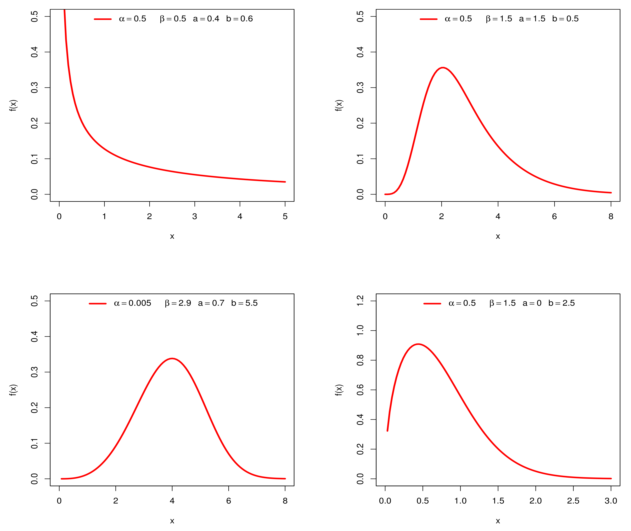
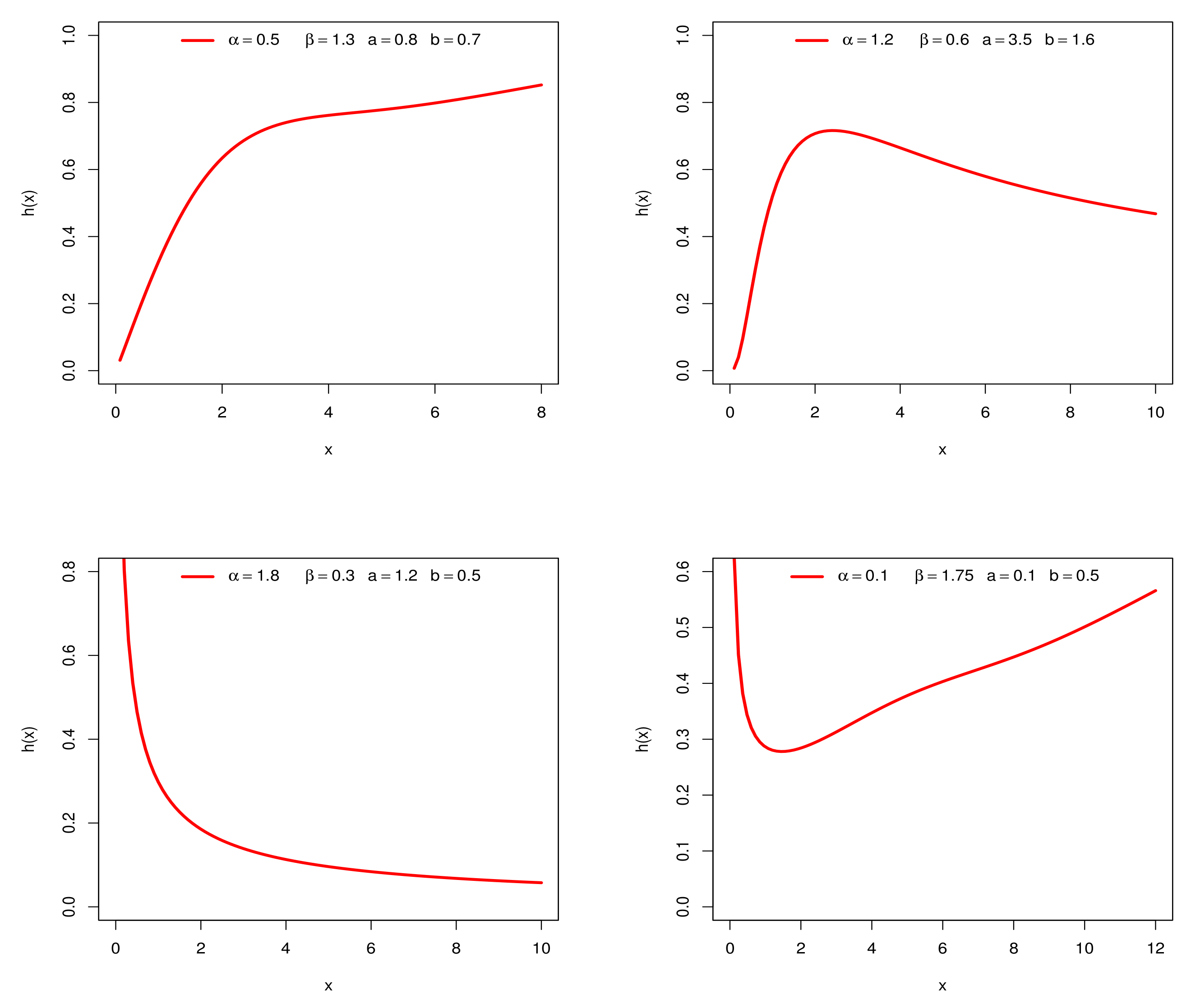
3.3. Analytic Shapes of the Density and Hazard Rate Function

The shapes of the density and hrf of X can be described analytically. The critical points of the density of X are the roots of the equation:

$$\begin{array}{ccc}& & \frac{g^{\prime }(x;\xi )}{g(x;\xi )}-\frac{G(x;\xi )g(x;\xi )}{\overline{G}(x;\xi )}+\frac{g(x;\xi )\left\{G(x;\xi )-2\right\}}{\{G(x;\xi )-1\}\left[G(x;\xi )+\{G(x;\xi )-1\}log\overline{G}(x;\xi )\right]}\hfill \\ & & +g(x;\xi )log\overline{G}(x;\xi )-\frac{(a-1)g(x;\xi )M\left[G(x;\xi )+\{G(x;\xi )-1\}log\overline{G}(x;\xi )\right]}{(M-1)\overline{G}(x;\xi )}\hfill \\ & & +\frac{a(b-1)g(x;\xi )M{\left(1-M\right)}^{a-1}\left[\frac{1}{G(x;\xi )-1}+log\overline{G}(x;\xi )+1\right]}{1-{\left(1-M\right)}^a}=0,\hfill \end{array}$$

where $M=M(x;\xi )={[1-G(x;\xi )]}^{G(x;\xi )}$.

The critical points of the hrf of X are obtained from the equation:

$$\begin{array}{ccc}& & \frac{g^{\prime }(x;\xi )}{g(x;\xi )}+\frac{1}{(M-1)\left[G(x;\xi )-1\right]\left[{(1-M)}^a-1\right]\left\{G(x;\xi )+\left[G(x;\xi )-1\right]log\overline{G}(x;\xi )\right\}}\hfill \\ & & \times g(x;\xi )[\left[1-{(1-M)}^a\right]\left[G(x;\xi )-1\right]\left\{-{log}^2\overline{G}(x;\xi )+G(x;\xi ){\left[log\overline{G}(x;\xi )+1\right]}^2+2\right\}\hfill \\ & & +M\{2-2{(1-M)}^a-a{log}^2\overline{G}(x;\xi )-aG{(x;\xi )}^2{\left[log\overline{G}(x;\xi )+1\right]}^2\hfill \\ & & +G(x;\xi )\left[{(1-M)}^a+2alog\overline{G}(x;\xi )\left\{log\overline{G}(x;\xi )+1\right\}-1\right]\left\}\right]=0.\hfill \end{array}$$

3.4. Linear Representation of the NKw-G Density

Here, we derive useful expansions for Equations (7) and (8) based on the concept of exponentiated distributions. For an arbitrary baseline cdf $G(x;\xi )$, a rv is said to have the exponentiated-G (exp-G) distribution with power parameter $a>0$ if its cdf and pdf are

$$H_a(x;\xi )=G{(x;\xi )}^a,h_a(x;\xi )=ag(x;\xi )G{(x;\xi )}^{a-1},$$

(10)

respectively.

The properties of the exponentiated distributions were studied by many authors in recent years. We consider the generalized binomial expansion

$${(1-z)}^b=\sum _{k=0}^{\infty }{(-1)}^k\left(\genfrac{}{}{0pt}{}{b}{k}\right)z^k,$$

(11)

which holds for any real non-integer b and $\left|z\right|<1$. Using (11) twice in the following expression $T(x;\xi )={\left\{1-{\left[1-P(x;\xi )\right]}^a\right\}}^b$ in Equation (7), where $P(x;\xi )=\overline{G}{(x;\xi )}^{G(x;\xi )}$, we can write $T(x;\xi )={\sum }_{j=0}^{\infty }{w}_{j+1}P{(x;\xi )}^{j+1}$, where $w_{j+1}={\sum }_{m=1}^{\infty }{(-1)}^{j+m+1}\left(\genfrac{}{}{0pt}{}{b}{m}\right)\left(\genfrac{}{}{0pt}{}{ma}{j+1}\right)$. Then, we can expand Equation (7) as

$$F\left(x\right)=1-\sum _{j=0}^{\infty }{w}_{j+1}{[1-G(x;\xi )]}^{(j+1)G(x;\xi )}.$$

(12)

Furthermore, using Mathematica, the power series holds

$${[1-G(x;\xi )]}^{(j+1)G(x;\xi )}=1+\sum _{i=2}^{\infty }{q}_i(j+1)G{(x;\xi )}^i,$$

(13)

where $q_2(j+1)=-(j+1)$, $q_3(j+1)=-(j+1)/2$, $q_4(j+1)=(j+1)(3j+1)/6$, $q_5(j+1)=(j+1)(2j+1)/4$, etc.

By inserting Equation (13) in Equation (12) and noting that ${\sum }_{j=0}^{\infty }{w}_{j+1}=1$, we obtain

$$F\left(x\right)=\sum _{i=2}^{\infty }{t}_{i}G{(x;\xi )}^i,$$

(14)

where

$$t_i=-\sum _{j=0}^{\infty }{w}_{j+1}{q}_i(j+1)\mathrm{for}i\ge 2.$$

(15)

By differentiating $F\left(x\right)$, the NKwG density has the form

$$f\left(x\right)=\sum _{i=1}^{\infty }{t}_{i+1}{h}_{i+1}(x;\xi ),$$

(16)

where $h_{i+1}(x;\xi )$ is the exp-G density with power parameter ($i+1$). Equation (16) reveals that the NKw-G density function is a linear combination of exp-G densities. Then, some of its mathematical properties can be determined directly from those of the exp-G distribution.

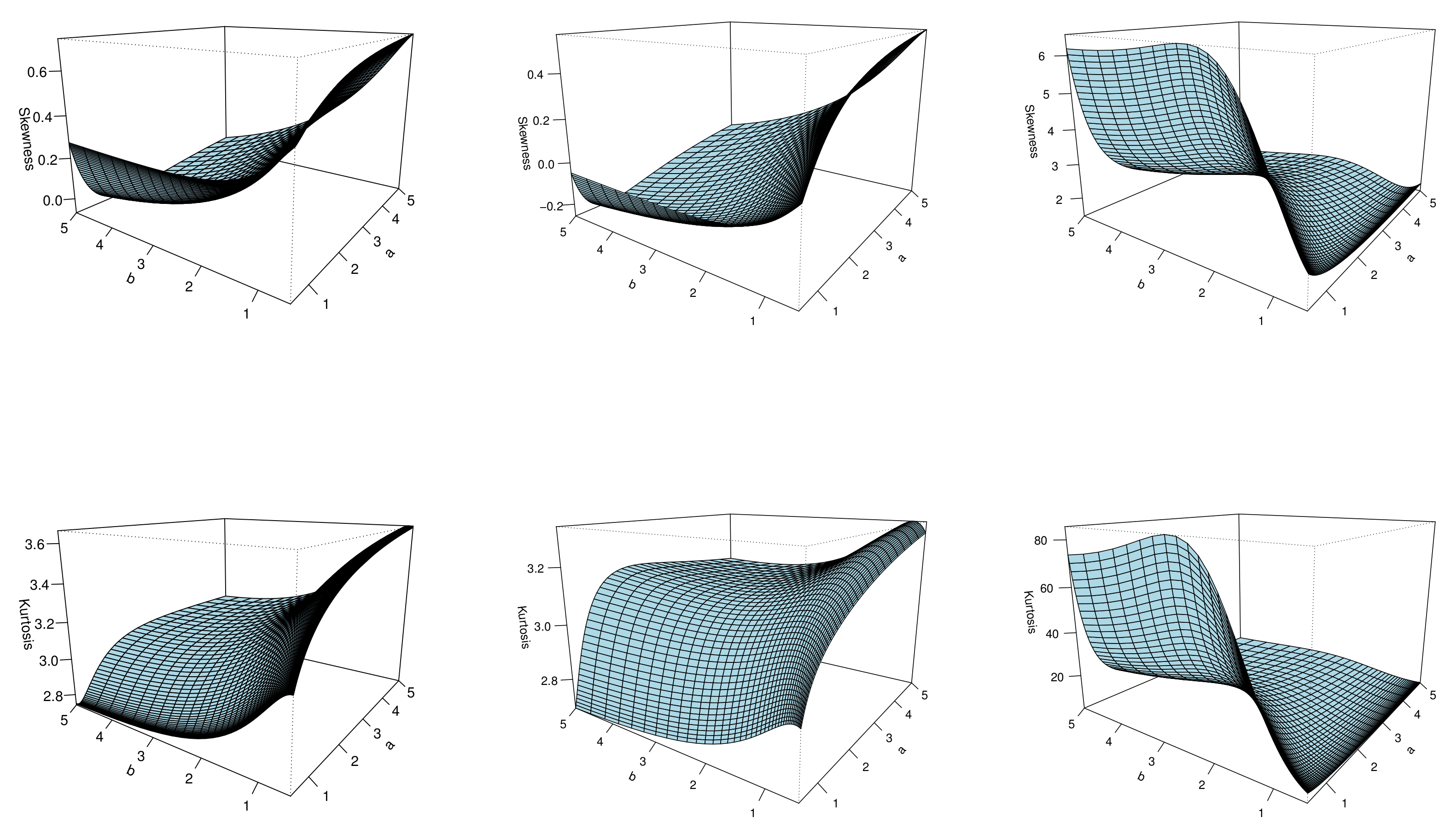
3.5. Mathematical Properties

The formulae derived throughout the paper can be easily handled in most symbolic computation platforms such as $\mathsf{Maple}$, $\mathsf{Mathematica}$ and $\mathsf{Matlab}$ which have the ability to deal with analytic expressions of formidable size and complexity. Henceforth, let $Y_{i+1}$ be a rv with the exp-G distribution with power parameter $(i+1)$. We obtain some mathematical quantities of the NKw-G family from (16) and those properties of the exp-G distribution. The exp-G properties are known for at least fifty distributions; see those distributions listed in Tahir and Nadarajah [16].

First, the nth ordinary moment of X, say $\mathbb{E}\left(X^n\right)$, can be expressed from (16) as

$$\mathbb{E}\left(X^n\right)=\sum _{i=1}^{\infty }{t}_{i+1}\mathbb{E}\left(Y_{i+1}^n\right)=\sum _{i=1}^{\infty }(i+1)t_{i+1}{\tau }_{n,i},$$

(17)

where ${\tau }_{n,i}={\int }_{-\infty }^{\infty }{x}^{n}G{(x;\xi )}^{i}g(x;\xi )dx={\int }_0^1{Q}_G{(u;\xi )}^n{u}^{i}du$, and $Q_G(u;\xi )$ is the qf of the baseline G. The quantities $\mathbb{E}\left(Y_{i+1}^n\right)$ are known for many G distributions as can been seen in those papers cited in Tahir and Nadarajah (2015).

Moments are important in any statistical analysis. Some of the most important features of a distribution can be studied through moments. For instance, the first four moments can be used to describe some characteristics of a distribution. Clearly, the central moments and cumulants of X can be determined from (17) using well-known relationships.

Second, the nth lower incomplete moment of X, say $m_n\left(y\right)={\int }_{-\infty }^y{x}^{n}f\left(x\right)dx$, is

$$\begin{array}{ccc}\hfill m_n\left(y\right)& =& \sum _{i=1}^{\infty }{t}_{i+1}{\int }_{-\infty }^y{x}^n{h}_{i+1}\left(x\right)dx=\sum _{i=1}^{\infty }(i+1)t_{i+1}{\int }_0^{G(y;\xi ))}{Q}_G{(u;\xi )}^n{u}^{i}du.\hfill \end{array}$$

(18)

The last two integrals can be evaluated numerically for most G distributions.

The first incomplete moment $m_1\left(y\right)$ is used to construct the Bonferroni and Lorenz curves (popular measures in economics, reliability, demography, insurance, and medicine) and to determine the totality of deviations from the mean and median of X (important statistics in statistical applications).

Third, for a given probability $\pi$, the Bonferroni and Lorenz curves (popular measures in economics, reliability, demography, insurance and medicine) of X are given by $B\left(\pi \right)=m_1\left(q\right)/\left(\pi {\mu }_1^{\prime }\right)$ and $L\left(\pi \right)=m_1\left(q\right)/{\mu }_1^{\prime }$, respectively, where $q=Q(\pi ;\xi )$ can be found from the procedure described at the last paragraph of Section 2.

Fourth, the total deviations from the mean and median are ${\delta }_1=2{\mu }_1^{\prime }F\left({\mu }_1^{\prime }\right)-2m_1\left({\mu }_1^{\prime }\right)$ and ${\delta }_2={\mu }_1^{\prime }-2m_1\left(M\right)$, where $F\left({\mu }_1^{\prime }\right)$ comes from (7).

Fifth, the moment generating function (mgf) $M\left(t\right)=\mathbb{E}\left({\mathrm{e}}^{\mathrm{t}\mathrm{X}}\right)$ of X follows from (16) as

$$\begin{array}{c}\hfill M\left(t\right)=\sum _{i=1}^{\infty }{t}_{i+1}{M}_{i+1}\left(t\right)=\sum _{i=0}^{\infty }(i+1)t_{i+1}{\rho }_i\left(t\right),\end{array}$$

(19)

where $M_{i+1}\left(t\right)$ is the mgf of $Y_{i+1}$ and ${\rho }_i\left(t\right)={\int }_0^{1}exp\left[t{Q}_G(u;\xi )\right]u^{i}du$. Hence, we can obtain the mgfs of many special NKw-G distributions directly from exp-G generating function and Equation (19).

3.6. Estimation

Here, we consider the estimation of the unknown parameters of the NKw-G family by the maximum likelihood method. The MLEs enjoy desirable properties and deliver simple approximations that work well in finite samples when constructing confidence intervals. The normal approximation for the MLEs can be handled either analytically or numerically.

The log-likelihood function $\ell \left(\theta \right)$ for the vector of parameters $\theta ={(a,b,\xi )}^{\top }$ from n observations $x_1,\cdots ,x_n$ has the form

$$\begin{array}{ccc}\hfill \ell =\ell \left(\theta \right)& =& nlog\left(ab\right)+\sum _{i=1}^{n}log\left[g(x_i;\xi )\right]+\sum _{i=1}^{n}G(x_i;\xi )log[1-G(x_i;\xi )]\hfill \\ & & +(a-1)\sum _{i=1}^{n}log\left\{1-{[1-G(x_i;\xi )]}^{G(x_i;\xi )}\right\}\hfill \\ & & +(b-1)\sum _{i=1}^{n}log\left[1-{\left\{1-{[1-G(x_i;\xi )]}^{G(x_i;\xi )}\right\}}^a\right]\hfill \\ & & +\sum _{i=1}^{n}log\left[\frac{G(x_i;\xi )}{1-G(x_i;\xi )}-log[1-G(x_i;\xi )]\right].\hfill \end{array}$$

The MLE $\widehat{\theta }$ of $\theta$ can be evaluated by maximizing $\ell \left(\theta \right)$. There are several routines for numerical maximization of $\ell \left(\theta \right)$ in the R program (optim function), SAS (PROC NLMIXED), Ox (sub-routine MaxBFGS), among others.

All distributions belonging to the NKw-G family can be fitted to real data using the AdequacyModel package for the R statistical computing environment (https://www.r-project.org/). An important advantage of this package is that it is not necessary to define the log-likelihood function and that it computes the MLEs, their standard errors and some GoF statistics. We only need to provide the pdf and cdf of the distribution to be fitted to a data set.

Alternatively, we can differentiate the log-likelihood and solving the resulting nonlinear likelihood equations. Then, the score components with respect to a, b and $\xi$ are

$$\begin{array}{ccc}\hfill \frac{\partial \ell }{\partial a}& =& \frac{n}{a}+\sum _{i=1}^{n}log\left\{1-{[1-G(x_i;\xi )]}^{G(x_i;\xi )}\right\}\hfill \\ & & -(b-1)\sum _{i=1}^n\frac{{\left\{1-{[1-G(x_i;\xi )]}^{G(x_i;\xi )}\right\}}^{a}log\left\{1-{[1-G(x_i;\xi )]}^{G(x_i;\xi )}\right\}}{1-{\left[1-{(1-G(x_i;\xi ))}^{G(x_i;\xi )}\right]}^a},\hfill \\ \hfill \frac{\partial \ell }{\partial b}& =& \frac{n}{b}+\sum _{i=1}^{n}log\left[1-{\left\{1-{[1-G(x_i;\xi )]}^{G(x_i;\xi )}\right\}}^a\right],\hfill \\ \hfill \frac{\partial \ell }{\partial \xi }& =& \sum _{i=1}^n\frac{g_i^{\xi }}{g(x_i;\xi )}-\sum _{i=1}^n\left\{\frac{G(x_i;\xi )}{1-G(x_i;\xi )}-log(1-G(x_i;\xi ))\right\}{G}_i^{\xi }\hfill \\ & & -\sum _{i=1}^n\frac{G_i^{\xi }\left[G(x_i;\xi )-2\right]}{(1-G(x_i;\xi ))\left[-log\{1-G(x_i;\xi )\}+G(x_i;\xi )\left\{1+log(1-G(x_i;\xi ))\right\}\right]}\hfill \\ & & +(a-1)\sum _{i=1}^n\frac{{\left(1-G(x_i;\xi )\right)}^{G(x_i;\xi )-1}}{{[1-G(x_i;\xi )]}^{G(x_i;\xi )}}[-log\{1-G(x_i;\xi )\}+G(x_i;\xi )\hfill \\ & & \times \left\{1+log(1-G(x_i;\xi ))\right\}]G_i^{\xi }-(b-1)\sum _{i=1}^n\frac{a{\left\{1-{(1-G(x_i;\xi ))}^{G(x_i;\xi )}\right\}}^{a-1}}{1-{\left[1-{(1-G(x_i;\xi ))}^{G(x_i;\xi )}\right]}^a}\hfill \\ & & \times {\left(1-G(x_i;\xi )\right)}^{G(x_i;\xi )-1}\left[-log\{1-G(x_i;\xi )\}+G(x_i;\xi )\left\{1+log(1-G(x_i;\xi ))\right\}\right]G_i^{\xi },\hfill \end{array}$$

where $g_i^{\xi }=\frac{\partial g(x_i;\xi )}{\partial \xi }$ and $G_i^{\xi }=\frac{\partial G(x_i;\xi )}{\partial \xi }$ are column vectors of the same dimension of $\xi$.

Setting the score components to zero and solving them simultaneously yields the MLEs of the model parameters. The resulting equations cannot be solved analytically, but some statistical softwares can be used to solve them numerically through iterative Newton-Raphson type algorithms.

For interval estimation and hypothesis tests on the model parameters, we can obtain the $(p+2)\times (p+2)$ observed information matrix $J\left(\theta \right)$ numerically (p is the dimension of $\xi$) since the expected information matrix $K\left(\theta \right)$ is very complicated and requires numerical integration.

Under standard regularity conditions, we have $(\widehat{\theta }-\theta )\stackrel{a}{\sim }{\mathcal{N}}_{p+2}(\mathbf{0},K{\left(\theta \right)}^{-1})$, where $\stackrel{a}{\sim }$ means approximately distributed and $K\left(\theta \right)$ is the expected information matrix. The asymptotic behavior remains valid if $K\left(\theta \right)$ is replaced by the observed information matrix $J\left(\theta \right)$ evaluated at $\widehat{\theta }$, i.e., $J\left(\widehat{\theta }\right)$. The multivariate normal ${\mathcal{N}}_{p+2}(\mathbf{0},J{\left(\widehat{\theta }\right)}^{-1})$ distribution can be used to construct approximate confidence intervals for the model parameters.

4. The NKwW Distribution

We now define the NKwW distribution by taking the Weibull baseline with cdf $G\left(x\right)=1-exp(-\alpha x^{\beta })$ and pdf $g\left(x\right)=\alpha \beta x^{\beta -1}exp(-\alpha x^{\beta })$. Then, the cdf and pdf of the NKwW distribution are, respectively, given by

$$\begin{array}{ccc}\hfill F_{NKwW}\left(x\right)& =& 1-{\left\{1-{\left[1-exp\left\{-\alpha x^{\beta }\left(1-exp(-\alpha x^{\beta })\right)\right\}\right]}^a\right\}}^b\hfill \end{array}$$

(20)

and

$$\begin{array}{ccc}\hfill f_{NKwW}\left(x\right)& =& ab\alpha \beta x^{\beta -1}exp\left\{-\alpha x^{\beta }\left(2-exp(-\alpha x^{\beta })\right)\right\}\hfill \\ & & \times {\left[1-exp\left\{-\alpha x^{\beta }\left(1-exp(-\alpha x^{\beta })\right)\right\}\right]}^{a-1}\hfill \\ & & \times {\left\{1-{\left[1-exp\left\{-\alpha x^{\beta }\left(1-exp(-\alpha x^{\beta })\right)\right\}\right]}^a\right\}}^{b-1}\hfill \\ & & \times \left[\frac{1-exp(-\alpha x^{\beta })}{exp(-\alpha x^{\beta })}+\alpha x^{\beta }\right].\hfill \end{array}$$

(21)

Henceforth, a rv with density (21) is denoted by $X\sim NKwW(a,b,\alpha ,\beta )$. The hrf of X has the form

$$\begin{array}{ccc}\hfill h\left(x\right)& =& ab\alpha \beta x^{\beta -1}exp\left\{-\alpha x^{\beta }\left(2-exp(-\alpha x^{\beta })\right)\right\}\hfill \\ & & \times {\left[1-exp\left\{-\alpha x^{\beta }\left(1-exp(-\alpha x^{\beta })\right)\right\}\right]}^{a-1}\hfill \\ & & \times {\left\{1-{\left[1-exp\left\{-\alpha x^{\beta }\left(1-exp(-\alpha x^{\beta })\right)\right\}\right]}^a\right\}}^{-1}\hfill \\ & & \times \left[\frac{1-exp(-\alpha x^{\beta })}{exp(-\alpha x^{\beta })}+\alpha x^{\beta }\right].\hfill \end{array}$$

Figure 1 and Figure 2 display some plots of the pdf and hrf of X for selected parameter values. Figure 1 reveals that the NKwW distribution is right-skewed and reversed-J shaped. Also, Figure 2 shows that the NKwW hrf can produce increasing, decreasing, bathtub and upside-down bathtub shapes.

4.1. Linear Representation

The cdf of the NKwW distribution follows from Equation (14) is

$$F_{NKwW}\left(x\right)=\sum _{i=2}^{\infty }{t}_i{\left[1-exp(-\alpha x^{\beta })\right]}^i.$$

(22)

By expanding the binomial term in (22) and noting that ${\sum }_{i=2}^{\infty }{t}_i=1$, we can write

$$F_{NKwW}\left(x\right)=1+\sum _{i=2}^{\infty }{t}_i\sum _{p=1}^i{(-1)}^p\left(\genfrac{}{}{0pt}{}{i}{p}\right)exp(-p\alpha x^{\beta })$$

and then by changing the index p by $(p+1)$ we get

$$F_{NKwW}\left(x\right)=1+\sum _{i=2}^{\infty }{t}_i\sum _{p=0}^i{(-1)}^{p+1}\left(\genfrac{}{}{0pt}{}{i}{p+1}\right)exp[-(p+1)\alpha x^{\beta }].$$

Let ${\delta }_p=2$ for $p=0,1,2$ and ${\delta }_p=p$ for $p\ge 3$. We can interchange the sums conveniently to obtain

$$F_{NKwW}\left(x\right)=1+\sum _{p=0}^{\infty }(-v_p)exp[-(p+1)\alpha x^{\beta }],$$

where $v_p={(-1)}^p{\sum }_{i={\delta }_p}^{\infty }\left(\genfrac{}{}{0pt}{}{i}{p+1}\right)t_i$.

By differentiating the last expression, the NKwW density can be expressed as

$$f_{NKwW}\left(x\right)=\sum _{p=0}^{\infty }{v}_p\pi (x;(p+1)\alpha ,\beta ),$$

(23)

where

$$\pi (x;(p+1)\alpha ,\beta )=(p+1)\alpha \beta x^{\beta -1}exp(-(p+1)\alpha x^{\beta })$$

denotes the Weibull density with scale parameter $(p+1)\alpha$ and shape parameter $\beta$.

Equation (23) shows that the NKwW density is a linear combination of Weibull densities. Therefore, several NKwW mathematical properties can be derived from those of the Weibull distribution.

4.2. Properties

Let $Z_p$ be a rv with density $\pi (x;(p+1)\alpha ,\beta )$. Then, several properties of X can follow from those of $Z_p$. First, the nth ordinary moment of X can be written as

$${\mu }_n^{\prime }=\Gamma \left(\frac{n}{\beta }+1\right)\sum _{p=0}^{\infty }\frac{v_p}{{\left[(p+1)\alpha \right]}^{n/\beta }}.$$

(24)

Second, the cumulants (${\kappa }_n$) of X can be determined recursively from (24) as ${\kappa }_s={\mu }_s^{\prime }-{\sum }_{k=1}^{s-1}\left(\genfrac{}{}{0pt}{}{s-1}{k-1}\right){\kappa }_k{\mu }_{s-k}^{\prime }$, respectively, where ${\kappa }_1={\mu }_1^{\prime }$.

The skewness ${\gamma }_1={\kappa }_3/{\kappa }_2^{3/2}$ and kurtosis ${\gamma }_2={\kappa }_4/{\kappa }_2^2$ of X can be calculated from the third and fourth standardized cumulants. The skewness and kurtosis plots of the NKwW distribution are displayed in Figure 3. These plots reveal that the parameters a and b play a significant role in modeling the skewness and kurtosis behaviors of X.

Third, we derive an approximation for the density of the sample average $\overline{X}={\sum }_{i=1}^n{X}_i/\sqrt{n}$ of independent and identically (iid) rvs $X_1,\cdots ,X_n$ with density (21). Without loss of generality, we can replace each $X_i$ by $(X_i-{\mu }_1^{\prime })/\mathrm{Var}\left(X_i\right)$ in order to simplify the approximation. By doing this, the previous third and fourth standardized cumulants are ${\gamma }_1={\mu }_3^{\prime }$ and ${\gamma }_2={\mu }_4^{\prime }-3$. Furthermore, we require the first six Hermite polynomials defined by ${(-1)}^n{\partial }^n\varphi \left(x\right)/\partial x^n=H_r\left(x\right)\varphi \left(x\right)$ for $n\ge 0$, where $\varphi \left(x\right)$ is the standard normal pdf. They satisfy the recurrence equation $H_r\left(x\right)=y{H}_{r-1}\left(x\right)-(r-1)H_{r-2}\left(x\right)(r\ge 2)$ and follow as $H_0\left(x\right)=1,H_1\left(x\right)=x,H_2\left(x\right)=x^2-1,H_3\left(x\right)=x^3-3x,H_4\left(x\right)=x^4-6x^2+3,H_5\left(x\right)=x^5-10x^3+15x$ and $H_6\left(x\right)=x^6-15x^4+45x^2-15$.

The second-order Edgeworth expansion for the sample mean $\overline{X}$ of standardized NKwW rvs can be expressed as

$$f_{\overline{X}}\left(x\right)=\varphi \left(x\right)\left\{1+\frac{{\mu }_3^{\prime }}{6\sqrt{n}}{H}_3\left(x\right)+\frac{({\mu }_4^{\prime }-3)}{24n}{H}_4\left(x\right)+\frac{{\mu }_3^{\prime 2}}{72n}{H}_6\left(x\right)\right\}+O\left(n^{-3/2}\right).$$

(25)

It is much more frequent in statistical applications to compute distribution functions than density functions. By integrating Equation (25), the cdf of $\overline{X}$ has the form

$$F_{\overline{X}}\left(x\right)=\Phi \left(x\right)-\varphi \left(x\right)\left\{\frac{{\mu }_3^{\prime }}{6\sqrt{n}}{H}_2\left(x\right)+\frac{({\mu }_4^{\prime }-3)}{24n}{H}_3\left(x\right)+\frac{{\mu }_3^{\prime 2}}{72n}{H}_5\left(x\right)\right\}+O\left(n^{-3/2}\right),$$

(26)

where $\Phi \left(x\right)$ is the standard normal cdf. Equation (26) provides highly accurate results for the probabilities associated with $\overline{Y}$.

Fourth, the nth incomplete moment of X, denoted by $m_n\left(y\right)=\mathbb{E}(X^n\mid X\le y)={\int }_0^y{x}^n{f}_{NKwW}\left(x\right)dx$, can easily be obtained by changing variables from the lower incomplete gamma function $\gamma (s,x)={\int }_0^{\infty }{x}^{s-1}{\mathrm{e}}^{-\mathrm{x}}\mathrm{dx}$ when calculating the corresponding moment of $Z_p$. Then, we obtain

$$m_n\left(z\right)=\sum _{p=0}^{\infty }\frac{v_p}{{\left[(p+1)\alpha \right]}^{n/\beta }}\gamma \left(\frac{n}{\beta }+1,(p+1)\alpha z^{\beta }\right).$$

(27)

Fifth, the first incomplete moment $m_1\left(z\right)$ is used to to determine the totality of deviations from the mean and median of a distribution and construct the Bonferroni and Lorenz curves. The total deviations from the mean and median M of X can be expressed as ${\delta }_1=2{\mu }_1^{\prime }{F}_{NKwW}\left({\mu }_1^{\prime }\right)-2m_1\left({\mu }_1^{\prime }\right)$ and ${\delta }_2={\mu }_1^{\prime }-2m_1\left(M\right)$, where M can be determined from $F_{NKwW}\left(M\right)=0.5$. The Bonferroni and Lorenz curves of X for a given probability $\pi$ are given by $B\left(\pi \right)=m_1\left(q\right)/\left(\pi m{u}_1^{\prime }\right)$ and $L\left(\pi \right)=\pi B\left(\pi \right)$, respectively, where $q=Q_{(}\pi )$ is the qf of X discussed in Section 4.1.

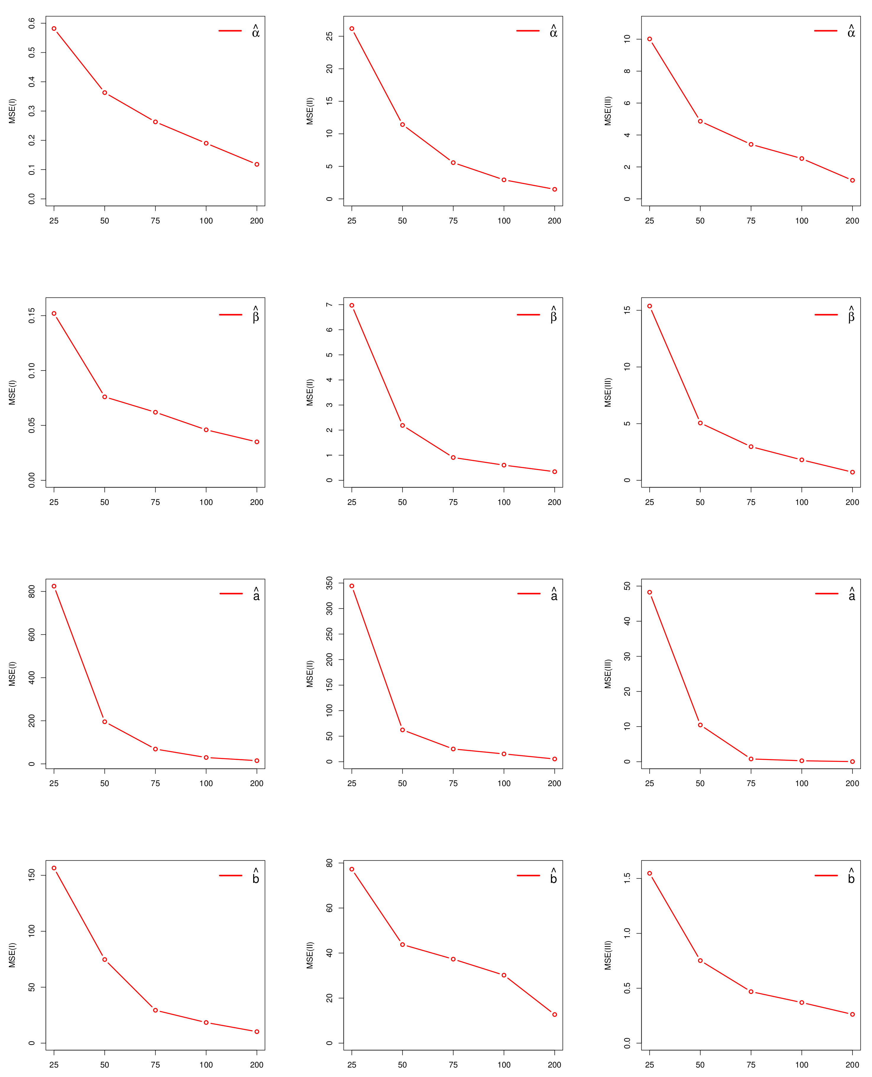
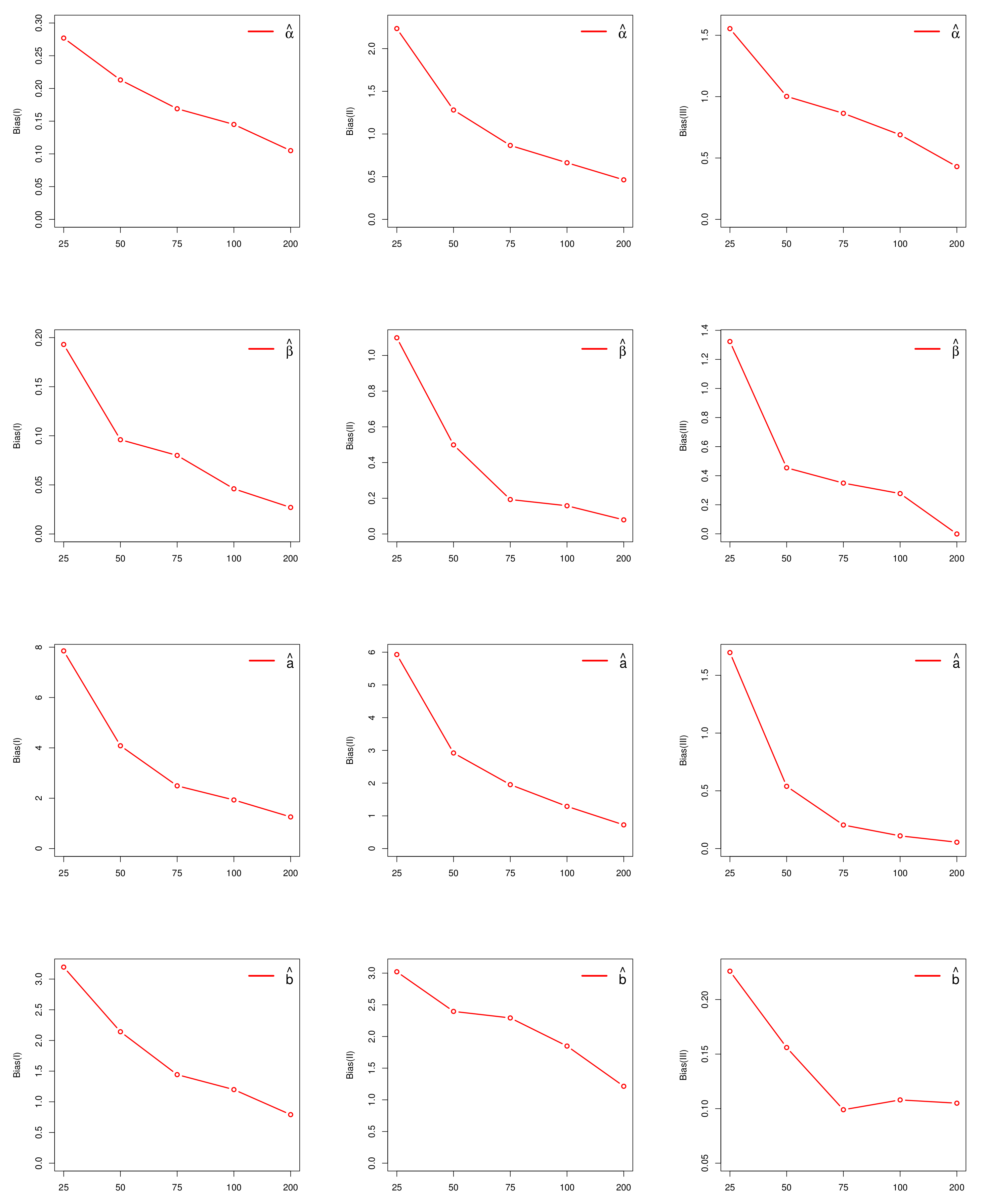
4.3. Quantile Function and Simulation Study

The qf of the NKwW distribution cannot be obtained explicitly. However, we can use Newton-Raphosn algorithm to generate NKwW variates as follows:

• Set n, $\alpha$, $\beta$, a, b and initial value $x^0$.
• Generate U ∼Uniform$(0,1)$.
• Update $x^0$ by using the Newton’s formula

  $$x*=x^0-R(x^0;\alpha ,\beta ,a,b),$$

  where $R(x^0;\alpha ,\beta ,a,b)=\frac{F_{NKwW}(x^0;\alpha ,\beta ,a,b)}{f_{NKwW}(x^0;\alpha ,\beta ,a,b)}$, and $F_{NKwW}$ and $f_{NKwW}$ are obtained from Equations (20) and (21), respectively.
• If $|x^0-x^{*}|\le ϵ$, ($ϵ>0$, very small tolerance limit), then store $x^0=x^{*}$ as a variate from the NKwW($\alpha ,\beta ,a,b$) distribution.
• If $|x^0-x^{*}|>ϵ$, then, set $x^0=x^{*}$ and go to step 3.
• Repeat steps (2)–(5) n times to generate $x_1,\cdots x_n$.

The R script to generate observations from the NKwW distribution is given in the Appendix A.

Here we study the performance and accuracy of maximum likelihood estimates of the NKwW parameters using Monte Carlo simulations. The simulation study is carried out for sample sizes $n=25,50,75,100,200$ and parameter scenarios: I: $\alpha =0.5$, $\beta =0.5$, $a=2.5$, and $b=1.5$, II: $\alpha =1.5$, $\beta =1.5$, $a=1.5$, and $b=1.5$ and III: $\alpha =1.1$, $\beta =5.5$, $a=0.5$, and $b=0.5$. We used the above algorithm for sample generation whose R-codes ae given in Appendix A. The simulation study is repeated for N = 1000 times each with given sample size and computed the average estimates (AE) along with their average biases (Bias)of the MLEs and mean squared errors (MSE).

$$Bias\left(\widehat{\theta }\right)=\sum _{i=1}^N\frac{\widehat{{\theta }_i}}{N}-\theta \mathrm{and}MSE\left(\widehat{\theta }\right)=\sum _{i=1}^N\frac{{(\widehat{{\theta }_i}-\theta )}^2}{N}.$$

We display Bias and MSE for the parameters $\alpha$, $\beta$, a and b in Figure 4 and Figure 5, respectively, which indicate that as sample size increases the bias and MSE decreases. Thus, MLEs perform well in estimating the parameters of the NKwW distribution.

4.4. Estimation

Let $x_1,\cdots ,x_n$ be a sample of size n from the NKwW distribution given in Equation (21). The log-likelihood function $\ell =\ell \left(\theta \right)$ for the vector of parameters $\theta ={(\alpha ,\beta ,a,b)}^{\top }$ is

$$\begin{array}{ccc}\hfill \ell & =& nlog\left(ab\alpha \beta \right)-2\alpha \sum _{i=1}^n{x}_i^{\beta }+\alpha \sum _{i=1}^n{x}_i^{\beta }exp(-\alpha x_i^{\beta })\hfill \\ & & +\sum _{i=1}^{n}log\left[\alpha x_i^{\beta }+exp(-\alpha x_i^{\beta })\left(1-exp(-\alpha x_i^{\beta })\right)\right]\hfill \\ & & +(\beta -1)\sum _{i=1}^{n}log{x}_i+(a-1)\sum _{i=1}^{n}log\left[1-exp(-\alpha x_i^{\beta })\left(1-exp(-\alpha x_i^{\beta })\right)\right]\hfill \\ & & +(b-1)\sum _{i=1}^{n}log\left[1-{\left\{1-exp(-\alpha x_i^{\beta })\left(1-exp(-\alpha x_i^{\beta })\right)\right\}}^a\right].\hfill \end{array}$$

The function ℓ can be easily maximized using the $\mathsf{AdequacyModel}$ package. The components of the score vector $U\left(\theta \right)$ are

$$\begin{array}{ccc}\hfill U_{\alpha }& =& \frac{n}{\alpha }+\sum _{i=1}^n\left(\frac{x_i^{\beta }\left[1+exp\left(\alpha x_i^{\beta }\right)\right]}{\alpha x_i^{\beta }+exp\left(\alpha x_i^{\beta }\right)-1}\right)-\sum _{i=1}^n{x}_i^{\beta }exp(-\alpha x_i^{\beta })\left[\alpha x_i^{\beta }+2exp\left(\alpha x_i^{\beta }\right)-1\right]\hfill \\ & & +(a-1)\sum _{i=1}^n\left(\frac{z_{i,\alpha }}{z_i}\right)-(b-1)\sum _{i=1}^n\left(\frac{a{z}_i^{a-1}{z}_{i,\alpha }}{1-z_i^a}\right),\hfill \\ \hfill U_{\beta }& =& \frac{n}{\beta }+\sum _{i=1}^{n}log{x}_i+\sum _{i=1}^n\left(\frac{\alpha x_i^{\beta }log\left(x\right)\left[1+exp\left(\alpha x_i^{\beta }\right)\right]}{\alpha x_i^{\beta }+exp\left(\alpha x_i^{\beta }\right)-1}\right)-\sum _{i=1}^n\left[\alpha x_i^{\beta }log\left(x\right)exp(-\alpha x_i^{\beta })\right]\hfill \\ & & \times \left[\alpha x_i^{\beta }+2exp\left(\alpha x_i^{\beta }\right)-1\right]+(a-1)\sum _{i=1}^n\left(\frac{z_{i,\beta }}{z_i}\right)-(b-1)\sum _{i=1}^n\left(\frac{a{z}_i^{a-1}{z}_{i,\beta }}{1-z_i^a}\right),\hfill \\ \hfill U_a& =& \frac{n}{a}+\sum _{i=1}^{n}log{z}_i-(b-1)\sum _{i=1}^n\left(\frac{z_i^{a}log{z}_i}{1-z_i^a}\right),\hfill \\ \hfill U_b& =& \frac{n}{b}+\sum _{i=1}^{n}log\left(1-z_i^a\right),\hfill \end{array}$$

where $z_i=1-exp\left\{-\alpha x_i^{\beta }\left[1-exp(-\alpha x_i^{\beta })\right]\right\}$,

$z_{i\alpha }=x_i^{\beta }\left[\alpha x_i^{\beta }+exp\left(\alpha x_i^{\beta }\right)-1\right]exp\left\{-\alpha x_i^{\beta }\left[2-exp(-\alpha x_i^{\beta })\right]\right\}$,

$z_{i\beta }=\alpha x_i^{\beta }log{x}_i\left[\alpha x_i^{\beta }+exp\left(\alpha x_i^{\beta }\right)-1\right]exp\left\{-\alpha x_i^{\beta }\left[2-exp(-\alpha x_i^{\beta })\right]\right\}.$

The MLE $\widehat{\theta }$ of $\theta$ can be obtained by solving the nonlinear equations $U_{\alpha }=0$, $U_{\beta }=0$, $U_a=0$ and $U_b=0$. These equations cannot be solved analytically and statistical software can be used to obtain the estimates numerically. We can use iterative techniques such as a Newton-Raphson type algorithm to obtain $\widehat{\theta }$ using a wide range of initial values. The initial values for the parameters are important but are not hard to obtain from the fit of the Weibull distribution. This process often results or leads to more than one maximum. However, in these cases, we consider the MLEs corresponding to the largest value of the maximum. In a few cases, no maximum is identified for the selected initial values. In these cases, a new initial value is tried in order to obtain a maximum.

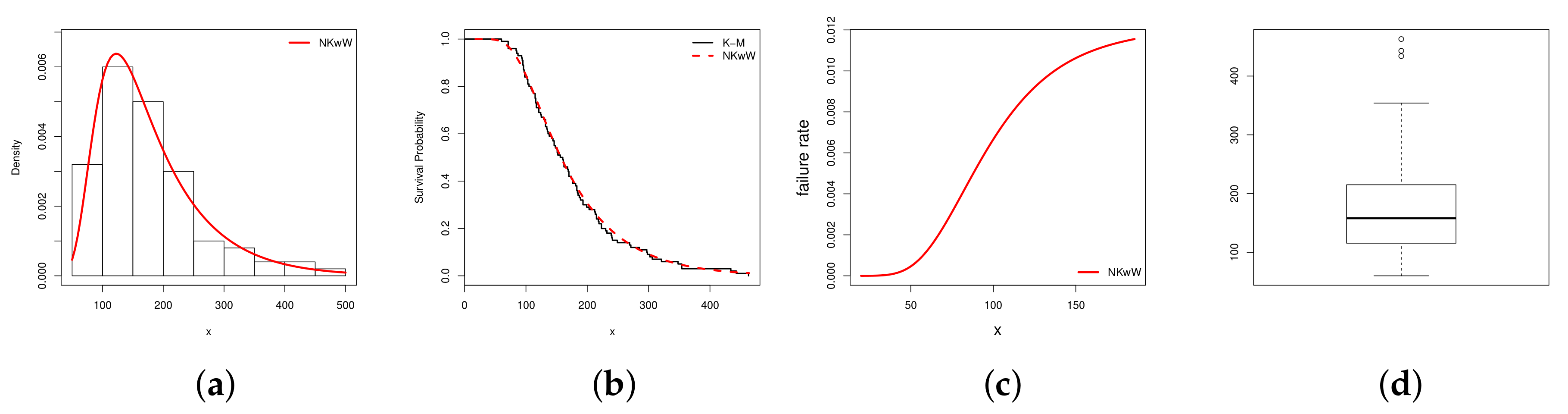
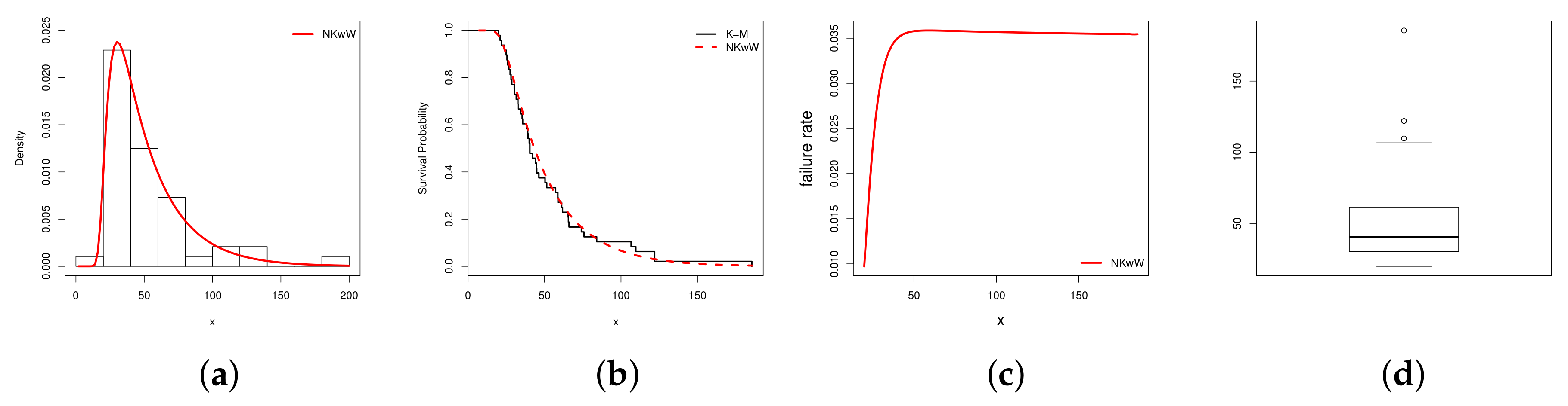
5. Empirical Illustrations of NKwW Model

In this section, we compare the NKwW distribution with some well-known extended (or generalized) Weibull distributions. To check the potentiality of the new distribution, we use two real data sets representing different hydrological events such as precipitation and flood. We compare the NKwW model with the Kumaraswamy-Weibull (KwW) (Cordeiro et al. [37]), beta-Weibull (BW) (Lee et al. [38]), exponentiated-generalized Weibull (EGW) (Oguntunde et al. [39]), McDonald-Weibull (McW) (Cordeiro et al. [40]), gamma-Weibull (GaW) (Cordeiro et al. [41]), odd log-logistc Weibull (OLLW) (da-Cruz et al. [42]), Marshall-Olkin Weibull (MOW) (Ghitany et al. [43]), transmuted-Weibull (TrW) (Khan et al. [44]) and Weibull (W) models by means of two real-life data sets which are described below:

Data Set 1. Precipitation data. The data were taken from Katz et al. [45] which represent the annual maximum precipitation (inches) for one rain gauge in Fort Collins, Colorado from 1900 through 1999. The data are: 239, 232, 434, 85, 302, 174, 170, 121, 193, 168, 148, 116, 132, 132, 144, 183, 223, 96, 298, 97, 116, 146, 84, 230, 138, 170, 117, 115, 132, 125, 156, 124, 189, 193, 71, 176, 105, 93, 354, 60, 151, 160, 219, 142, 117, 87, 223, 215, 108, 354, 213, 306, 169, 184, 71, 98, 96, 218, 176, 121, 161, 321, 102, 269, 98, 271, 95, 212, 151, 136, 240, 162, 71, 110, 285, 215, 103, 443, 185, 199, 115, 134, 297, 187, 203, 146, 94, 129, 162, 112, 348, 95, 249, 103, 181, 152, 135, 463, 183, 241.

Data set 2. Flood data. The data were taken from Asgharzadeh et al. [46] which represent the maximum annual flood discharges (in units of 1000 cubic feet per second) of the North Saskachevan River at Edmonton, over a period of 48 years. The data are: 19.885, 20.940, 21.820, 23.700, 24.888, 25.460, 25.760, 26.720, 27.500, 28.100, 28.600, 30.200, 30.380, 31.500, 32.600, 32.680, 34.400, 35.347, 35.700, 38.100, 39.020, 39.200, 40.000, 40.400, 40.400, 42.250, 44.020, 44.730, 44.900, 46.300, 50.330, 51.442, 57.220, 58.700, 58.800, 61.200, 61.740, 65.440, 65.597, 66.000, 74.100, 75.800, 84.100, 106.600, 109.700, 121.970, 121.970, 185.560.

All the calculations in these two applications are performed using the $\mathsf{AdequacyModel}$ package in R. The unknown parameters of the models are estimated by the maximum likelihood method. The log-likelihood function is evaluated at the MLEs ($\widehat{\ell }$). The well-known GoFS such as the Akaike information criterion (AIC), Bayesian Information Criterion (BIC), Hannan-Quinn Information Criterion (HQIC), Anderson-Darling ($A^{*}$), Cramér–von Mises ($W^{*}$) and Kolmogrov-Smirnov (K-S) are adopted for model comparisons. The lower values of GoFS and higher p-values of the K-S statistic indicate good fits.

Table 1. MLEs and their SEs (in parentheses) for data set 1.

Distribution	$\mathit{\alpha }$	$\mathit{\beta }$	a	b	$\mathit{\theta }$
NKwW	0.0089	1.1514	5.0192	0.5054	–
	(0.0023)	(0.0730)	(1.6716)	(0.1807)	–
KwW	0.0160	1.3962	5.7590	0.3381	–
	(0.0027)	(0.2113)	(1.9264)	(0.1554)	–
BW	0.0219	0.7969	13.2183	1.2340	–
	(0.0076)	(0.1903)	(5.1706)	(0.9787)	–
EGW	0.0086	0.9045	2.0898	10.5512	–
	(0.0022)	(0.1288)	(0.6257)	(4.4416)	–
McW	0.0132	1.2859	1.7925	0.5887	2.5824
	(0.0032)	(0.2544)	(0.6126)	(0.3831)	(0.9474)
GaW	1.1306	0.5469	17.6158	–	–
	(0.0496)	(0.0154)	(1.4970)	–	–
OLLW	0.0045	1.0313	2.4836	–	–
	(0.0003)	(0.1759)	(0.4532)	–	–
MOW	0.0032	3.4739	–	–	0.1039
	(0.0002)	(0.3436)	–	–	(0.0489)
TrW	0.0043	2.4549	–	–	0.6144
	(0.0003)	(0.1755)	–	–	(0.2078)
W	0.0050	2.2745	–	–	–
	(0.0002)	(0.1629)	–	–	–

and

Table 2. MLEs and their standard errors (in parentheses) for data set 2.

Distribution	$\mathit{\alpha }$	$\mathit{\beta }$	a	b	$\mathit{\theta }$
NKwW	0.1742	0.9887	59.0160	0.2183	–
	(0.0316)	(0.0619)	(0.4024)	(0.0585)	–
KwW	0.1609	1.0252	54.7825	0.2041	–
	(0.0153)	(0.0276)	(0.1358)	(0.0382)	–
BW	0.1320	1.1080	23.0602	0.1940	–
	(0.0073)	(0.0068)	(8.7941)	(0.0324)	–
EGW	0.0090	0.7774	5.5966	10.5493	–
	(0.0041)	(0.1370)	(2.0458)	(5.6821)	–
McW	0.1608	1.0049	14.5078	0.2210	2.5180
	(0.0340)	(0.0466)	(9.8227)	(0.0757)	(0.0895)
GaW	4.6144	0.4983	14.7225	–	–
	(0.1518)	(0.0217)	(1.7239)	–	–
OLLW	0.0154	0.9508	2.3925	–	–
	(0.0021)	(0.3378)	(0.9487)	–	–
MOW	0.0065	3.3556	–	–	0.0145
	(0.0014)	(0.4292)	–	–	(0.0146)
TrW	0.0137	1.9476	–	–	0.7003
	(0.0016)	(0.1941)	–	–	(0.2483)
W	0.0171	1.7719	–	–	–
	(0.0015)	(0.1776)	–	–	–

list the MLEs and their standard errors (SEs) for the NKwW distribution and other competitive models (KwW, BW, EGW, McW, GaW, OLLW, MOW, TrW and W) fitted to the two hydrological data sets. The values of the GoFS in

Table 3. The statistics AIC, BIC, HQIC, $A^{*}$, $W^{*}$, K-S and p-value for data set 1.

								K-S
Distribution	$\widehat{\mathit{\ell }}$	AIC	BIC	HQIC	${\mathit{A}}^{*}$	${\mathit{W}}^{*}$	K-S	P-Value
NKwW	565.2337	1138.4670	1148.8880	1142.6850	0.1722	0.0207	0.0454	0.9863
KwW	566.6253	1141.2510	1151.6710	1145.4680	0.3678	0.0477	0.0572	0.8987
BW	566.2292	1140.4580	1150.8790	1144.6760	0.3149	0.0411	0.0489	0.9707
EGW	566.2248	1140.4500	1150.8700	1144.6670	0.3266	0.0427	0.0487	0.9718
McW	567.4362	1144.8720	1157.8980	1150.1440	0.4868	0.0655	0.0596	0.8695
GaW	567.2618	1140.5240	1148.3390	1143.6870	0.5071	0.0689	0.0547	0.9257
OLLW	569.6909	1145.3820	1153.1970	1148.5450	0.6649	0.0932	0.0807	0.5335
MOW	568.4818	1142.9640	1150.7790	1146.1270	0.6431	0.0866	0.0595	0.8713
TrW	573.7855	1153.5710	1161.3870	1156.7340	1.4659	0.2183	0.0872	0.4321
W	576.1180	1156.2360	1161.4460	1158.3450	1.8275	0.2767	0.0936	0.3450

and

Table 4. The statistics AIC, BIC, HQIC, $A^{*}$, $W^{*}$, K-S and p-value for data set 2.

								K-S
Distribution	$\widehat{\mathit{\ell }}$	AIC	BIC	HQIC	${\mathit{A}}^{*}$	${\mathit{W}}^{*}$	K-S	P-Value
NKwW	215.1742	438.3485	445.8333	441.1770	0.2003	0.0277	0.0776	0.9346
KwW	215.5195	439.0389	446.5238	441.8675	0.2495	0.0347	0.0834	0.8924
BW	216.1573	440.3147	447.7995	443.1432	0.3387	0.0477	0.0973	0.7538
EGW	218.1801	444.3601	451.8449	447.1887	0.6147	0.0913	0.0973	0.7543
McW	215.7566	441.5132	450.8692	445.0489	0.2699	0.0374	0.0837	0.8895
GaW	219.4700	444.9401	450.5537	447.0615	0.8278	0.1250	0.1176	0.5203
OLLW	220.4104	446.8208	452.4344	448.9422	0.9051	0.1388	0.0934	0.7966
MOW	218.2594	442.5187	448.1323	444.6401	0.5773	0.0868	0.0791	0.9247
TrW	224.0997	454.1994	459.8130	456.3208	1.5006	0.2372	0.1291	0.4001
W	225.7065	455.4131	459.1555	456.8273	1.7286	0.2765	0.1399	0.3048

indicate that the NKwW model shows small values of these statistics and hence it provides the best fit as compared to the other models. The plots in Figure 6 and Figure 7 also support our claim.

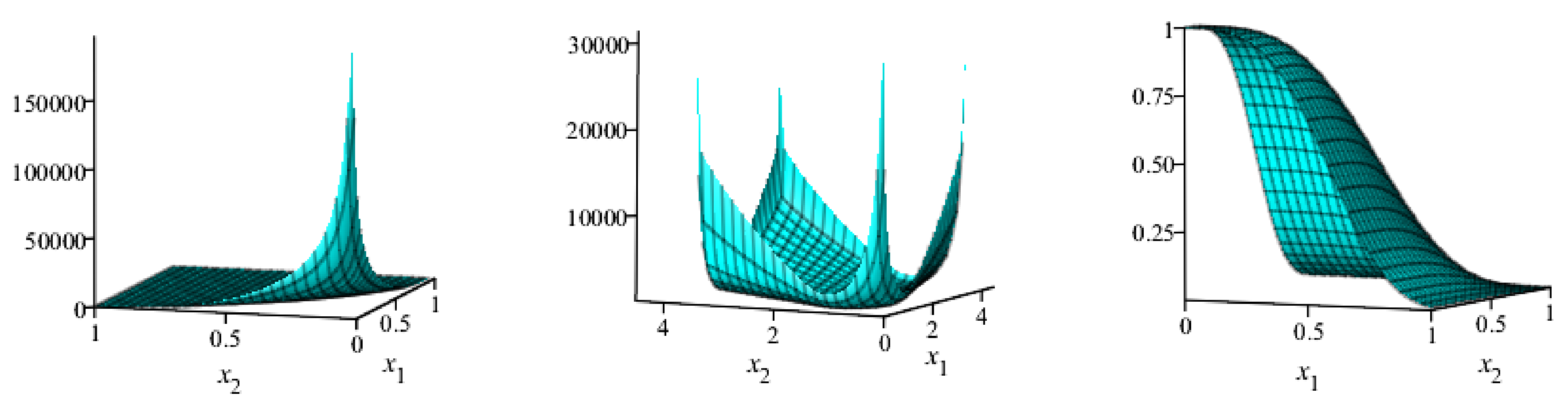
6. Bivariate New Kumaraswamy G-Family

In this Section, we introduce a bivariate extension of the NKw-G family according to Marshall and Olkin shock model (see, Marshall and Olkin, [47]). Several authors used the Marshall and Olkin approach as a method to generate bivariate distributions, see for example Sarhan and Balakrishnan, [48], Kundu and Dey [49], El-Gohary et al. [50], Muhammed [51], El-Bassiouny et al. [52], Ghosh and Hamedani [53], El-Morshedy et al. [54,55], Eliwa et al. [56], among others. The bivariate new Kumaraswamy (BvNKw) G-family is constructed from three independent NKw-G families by using a minimization process. Assume three independent rvs $Y_k\sim$NKw-G$(a,b_k,\xi );$$k=1,2,3$ and defining $X_j=min\{Y_j,Y_3\};j=1,2$, the bivaraite random vector $\mathbf{X}$ is said to have the BvNKw-G family with parameters vector ${\rm Y}=$($a,b_1,b_2$, $b_3,\xi$) if its joint reliability function (jrf) is given by

$$S_{X_1,X_2}(x_1,x_2;{\rm Y})=\left\{\begin{array}{c}{S}_{\mathrm{NKw}-\mathrm{G}}(x_1;a,b_1,\xi )S_{\mathrm{NKw}-\mathrm{G}}(x_2;a,b_2+b_3,\xi )\mathrm{if}{x}_1<x_2,\hfill \\ S_{\mathrm{NKw}-\mathrm{G}}(x_1;a,b_1+b_3,\xi )S_{\mathrm{NKw}-\mathrm{G}}(x_2;a,b_2,\xi )\mathrm{if}{x}_1\ge x_2.\hfill \end{array}\right.$$

(28)

The marginal reliability functions (rfs) corresponding to (28) can be written as

$$S_{X_i}\left(x_i\right)=S_{\mathrm{NKw}-\mathrm{G}}(x_i;a,b_i+b_3,\xi );i=1,2.$$

(29)

The corresponding joint pdf (jpdf) to (28) can be formulated as

$$f_{X_1,X_2}(x_1,x_2;{\rm Y})=\left\{\begin{array}{c}{f}_{\mathrm{NKw}-\mathrm{G}}(x_1;a,b_1,\xi )f_{\mathrm{NKw}-\mathrm{G}}(x_2;a,b_2+b_3,\xi )\mathrm{if}{x}_1<x_2,\hfill \\ f_{\mathrm{NKw}-\mathrm{G}}(x_1;a,b_1+b_3,\xi )f_{\mathrm{NKw}-\mathrm{G}}(x_2;a,b_2,\xi )\mathrm{if}{x}_1>x_2,\hfill \\ \frac{b_3}{b_1+b_2+b_3}{f}_{\mathrm{NKw}-\mathrm{G}}(x;a,b_1+b_2+b_3,\xi )\mathrm{if}{x}_1=x_2=x,\hfill \end{array}\right.$$

(30)

where the jpdf in Equation (30) can be derived from a well-known formula (see Eliwa and El-Morshedy, [57]). The marginal pdfs corresponding to Equation (29) can be proposed as

$$f_{X_i}\left(x_i\right)=f_{\mathrm{NKw}-\mathrm{G}}(x_i;a,b_i+b_3,\xi );i=1,2.$$

(31)

If $\mathbf{X}$ have the BvNKw-G family, then the distributions of $max\{X_1,X_2\}$ and $min\{X_1,X_2\}$ are

$$F_{max\{X_1,X_2\}}\left(w\right)=\prod _{i=1}^3{F}_{NKw-G}(w;a,b_i,\xi )\mathrm{and}{F}_{min\{X_1,X_2\}}\left(w\right)=1-\prod _{i=1}^3{S}_{\mathrm{NKw}-\mathrm{G}}(w;a,b_i,\xi ),$$

respectively. If $X_j\sim$NKw-G$(a,b_j+b_3,\xi );j=1,2$,then the coefficient of correlation between $X_1$ and $X_2$ is

$$Q{\left(u\right)}_{X_1,X_2}=\left\{\begin{array}{c}4F_{\mathrm{NKw}-\mathrm{G}}\left(Q{\left(u\right)}_{X_1};a,b_1,\xi \right)F_{\mathrm{NKw}-\mathrm{G}}\left(Q{\left(u\right)}_{X_2};a,b_2+b_3,\xi \right)-1\mathrm{if}{x}_1<x_2,\hfill \\ 4F_{\mathrm{NKw}-\mathrm{G}}\left(Q{\left(u\right)}_{X_1};a,b_1+b_3,\xi \right)F_{\mathrm{NKw}-\mathrm{G}}\left(Q{\left(u\right)}_{X_2};a,b_2,\xi \right)-1\mathrm{if}{x}_1>x_2.\hfill \end{array}\right.$$

(32)

The BvNKw-G family has a singular part along the line $x_1=x_2$ with weight $b_3{(b_1+b_2+b_3)}^{-1}$, whereas on $x_1\ne x_2$ with weight $(b_1+b_2){(b_1+b_2+b_3)}^{-1}$, the BvNKw-G family has an absolute continuous part. Assume ${\delta }_i$$=S_{X_i}\left(x_i\right)$ where $X_j\sim$NKw-G$(a,b_j+b_3,\xi );j=1,2$, the jrf of the proposed family can be derived by using copula of the Marshall-Olkin model as

$$S_{X_1,X_2}(x_1,x_2;{\rm Y})={\delta }_1^{1-{\tau }_1}{\delta }_2^{1-{\tau }_2}max\left({\delta }_1^{{\tau }_1},{\delta }_2^{{\tau }_2}\right),\mathrm{for}0<{\tau }_1,{\tau }_2<1,$$

where ${\tau }_j=\frac{b_3}{b_j+b_3}$. For more details on copula property, see Gijbels et al. [58] and Husková and Maciak [59].

Using Equations (28) and (30), the joint hrf (jhrf) can easily be reported by using $h_{X_1,X_2}(x_1,x_2;{\rm Y})=\frac{f_{X_1,X_2}(x_1,x_2;{\rm Y})}{S_{X_1,X_2}(x_1,x_2;{\rm Y})}$. Figure 8, Figure 9 and Figure 10 show the jpdf, jhrf, and jrf for different values of the BvNKw-Weibull (BvNKwW) parameters.

The MLE for the BvNKw-G Family

In this section, the unknown parameters of the BvNKw-G family are estimated by using the maximum likelihood approach. Assuming that $(x_{11},x_{21})$, $(x_{12},x_{22}),...,$$(x_{1p},x_{2p})$ is a sample of size p from the BvNKw-G family where ${\Lambda }_1=\{x_{1i}<x_{2i}\}$, ${\Lambda }_2=\{x_{1i}>x_{2i}\}$, ${\Lambda }_3=\{x_{1i}=x_{2i}=x_i\}$, $p_s=\left|{\Lambda }_s\right|;s=1,2,3$ and $\left|\Lambda \right|=p=p_1+p_2+p_3$. Using Equation (30), the likelihood function $l\left({\rm Y}\right)$ can be expressed as

$$\begin{array}{ccc}\hfill l\left({\rm Y}\right)& =& \prod _{i=1}^{p_1}{f}_{\mathrm{NKw}-\mathrm{G}}(x_{1i};a,b_1,\xi )f_{\mathrm{NKw}-\mathrm{G}}(x_{2i};a,b_2+b_3,\xi )\prod _{i=1}^{p_2}{f}_{\mathrm{NKw}-\mathrm{G}}(x_{1i};a,b_1+b_3,\xi )\hfill \\ & & \times f_{\mathrm{NKw}-\mathrm{G}}(x_{2i};a,b_2,\xi ){\left(\frac{b_3}{b_1+b_2+b_3}\right)}^{p_3}\prod _{i=1}^{p_3}{f}_{\mathrm{NKw}-\mathrm{G}}(x_i;a,b_1+b_2+b_3,\xi ).\hfill \end{array}$$

(33)

Through differentiation of the term $L\left(\mathrm{Y}\right)=log$$l\left(\mathrm{Y}\right)$ with respect to $a,b_1,b_2,b_3$ and $\xi$, and then equating the resulting equations to zeros, we get the non-linear normal equations. An iterative procedure such as Newton–Raphson technique is required to solve them numerically.

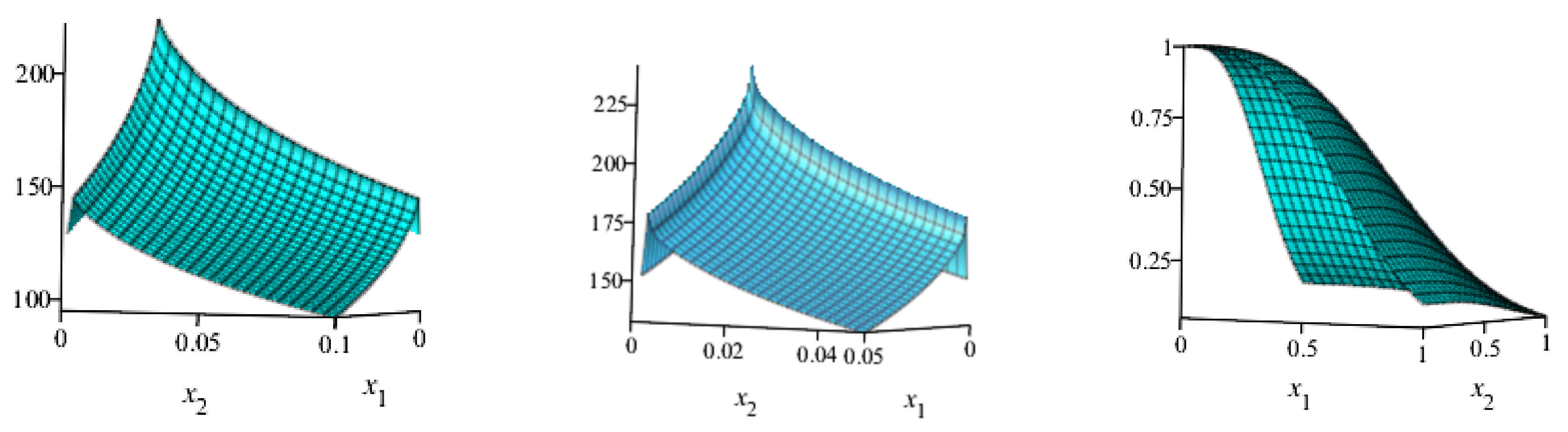
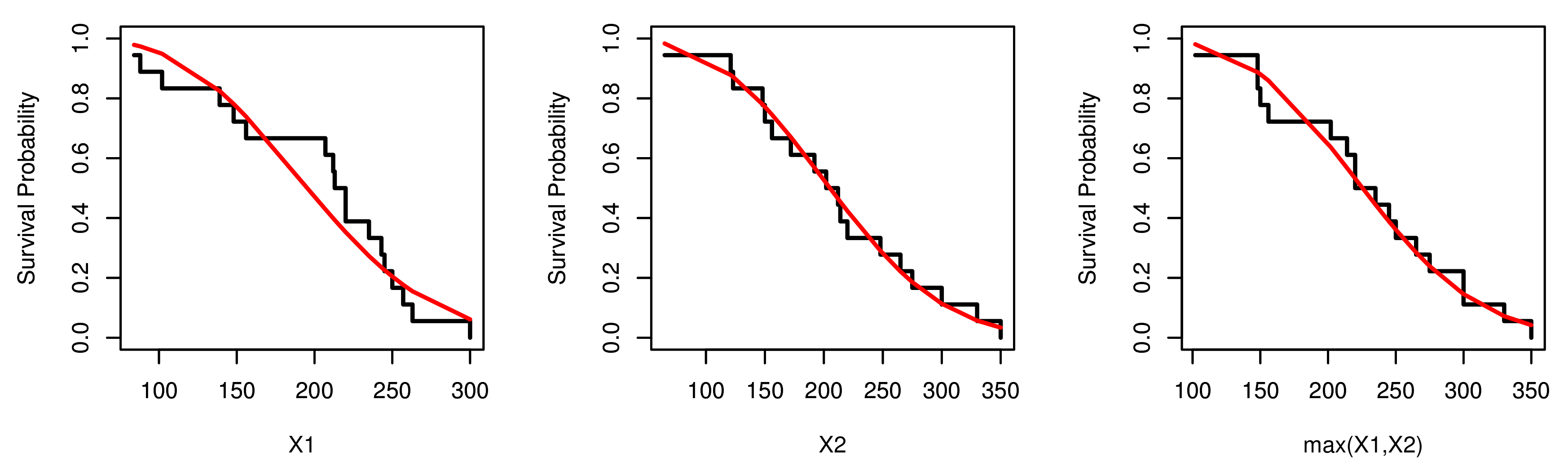
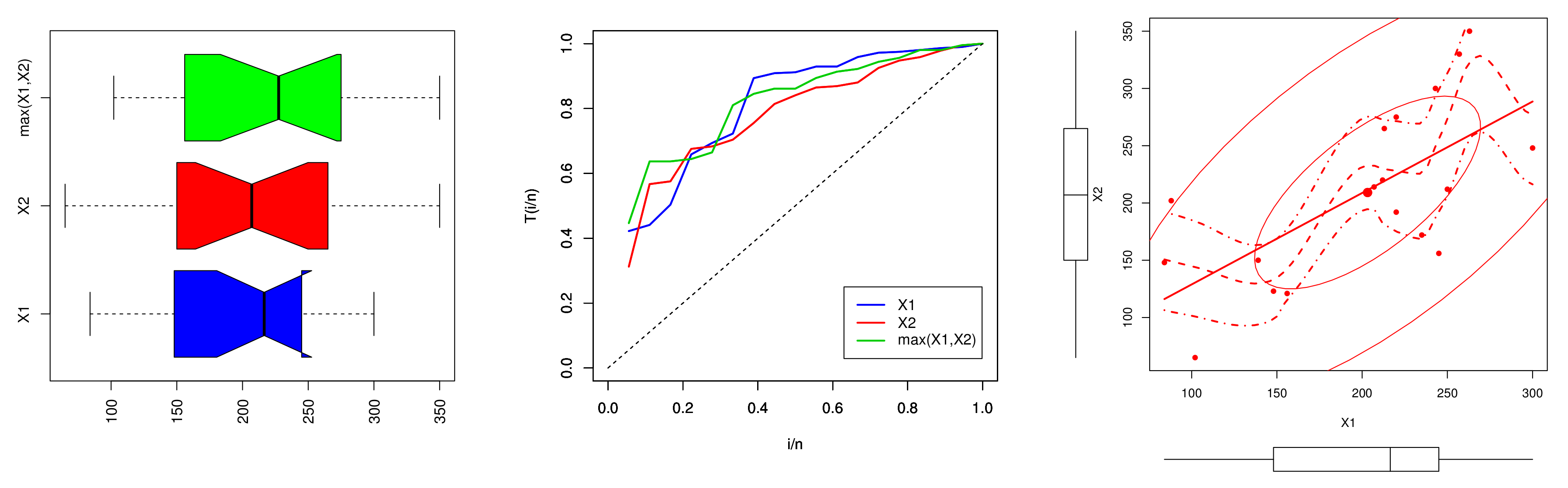
7. Empirical Illustrations of BvNKwW Model Through Motors Data

In this Section, the flexibility of the BvNKwW model is shown through a real-life data application. This data is reported in Relia and Staff [60] which represents the failure times of a parallel system constituted by two identical motors in days. The fitted bivariate models are compared using some statistical criteria, namely AIC, CAIC, BIC and HQIC. To fit the marginals of the BvNKwW model, the K-S with its p-value are used. The BvNKwW model is compared with other bivariate distributions such as: bivariate generalized power Weibull (BvGPW), bivariate exponentiated Weibull (BvEW), bivariate Weibull (BvW), bivariate generalized exponential (BvGEx), bivariate exponential (BvEx), and bivariate generalized linear failure rate (BvGLFR) distributions when applied to this data set. At first, the marginals $X_1$, $X_2$ and $max(X_1,X_2)$ are fitted separately to this data set. The MLEs of the parameters $(a,b,\alpha ,\beta )$ of the corresponding NKwW distribution for $X_1$, $X_2$ and $max(X_1,X_2)$ are ($60.5030$, $732.6059$, $0.9694$, $0.17440$), ($1.8182$, $84.4223$, $0.0019$, $0.9434$) and ($27.8306$, $263.4773$, $0.4649$, $0.2626$), respectively. The $-L$, K-S, p-value for the marginals are reported in

Table 5. The -L, K-S and p-values for $X_1$, $X_2$ and $max(X_1,X_2)$.

	${\mathit{X}}_1$			${\mathit{X}}_2$			$max({\mathit{X}}_1,{\mathit{X}}_2)$
Model	−L	K-S	P-Value	−L	K-S	P-Value	−L	K-S	P-Value
NKwW	$100.2890$	$0.2376$	$0.2614$	$102.9142$	$0.0902$	$0.9956$	$101.1965$	$0.1372$	$0.8871$

.

Table 5 lists that the NKwW model fits to the real data for the marginals. Figure 11, Figure 12 and Figure 13 show the fitted pdf, cdf and probability-probability (pp) plots, which support our empirical results in Table 5.

Figure 14 show the box and TTT plots for the $X_1$, $X_2$ and $max(X_1,X_2)$, and the scatter plot for the motors data.

It is noted that the BvNKwW model can be used to analyze and the real data on motors. The MLEs, $-L$, AIC, CAIC, BIC and HQIC values for the BvNKwW model and some competitive models are listed in

Table 6. The MLEs with its (SE) and goodness of fit measures for Motors data.

	Model
Statistic	BvNKwW	BvGPW	BvEW	BvW	BvGEx	BvEx	BvGLFR
$\widehat{a}$	$1.6395$	$0.0291$	$0.5203$	$0.0389$	$0.0137$	−	$6.99\times {10}^{-5}$
	$\left(0.0651\right)$	$\left(0.0557\right)$	$\left(0.0511\right)$	$\left(0.0158\right)$	$\left(0.0023\right)$	−	$\left(1.09\times {10}^{-5}\right)$
$\widehat{b_1}$	$3.1333$	1.5591	30.1381	0.2004	2.4541	0.0023	0.4171
	$\left(0.2364\right)$	$\left(3.0428\right)$	$\left(9.6756\right)$	$\left(0.0511\right)$	$\left(1.0189\right)$	$\left(0.0005\right)$	$\left(9.71\times {10}^{-7}\right)$
$\widehat{b_2}$	$3.3989$	$1.8581$	$24.1351$	$0.2383$	$2.8803$	$0.0021$	$0.4864$
	$\left(0.1896\right)$	$\left(3.6787\right)$	$\left(7.6763\right)$	$\left(0.0513\right)$	$\left(1.1158\right)$	$\left(0.0005\right)$	$\left(1.05\times {10}^{-6}\right)$
$\widehat{b_3}$	$4.2869$	$3.7191$	$61.8051$	$0.3381$	$6.0641$	$0.0051$	$1.0188$
	$\left(0.0985\right)$	$\left(7.2630\right)$	$\left(6.3779\right)$	$\left(0.0622\right)$	$\left(1.8113\right)$	$\left(0.0009\right)$	$\left(1.33\times {10}^{-6}\right)$
$\widehat{\alpha }$	$0.0008$	$0.0291$	$0.5203$	$0.0389$	$0.0137$	−	$6.99\times {10}^{-5}$
	$\left(0.0001\right)$	$\left(0.0557\right)$	$\left(0.0511\right)$	$\left(0.0158\right)$	$\left(0.0023\right)$	−	$\left(1.09\times {10}^{-5}\right)$
$\widehat{\beta }$	$1.2532$	−	−	−	−	−	−
	$\left(0.3421\right)$	−	−	−	−	−	−
$-L$	$211.1711$	$431.7909$	$339.2656$	$422.9532$	$335.2312$	$355.7323$	$331.7681$
AIC	$434.3422$	$871.5818$	$688.5312$	$853.9064$	$678.4624$	$717.4646$	$673.5362$
CAIC	$441.9786$	$874.6587$	$693.5312$	$856.9833$	$681.5393$	$719.1789$	$678.5362$
BIC	$439.6844$	$875.14328$	$692.9831$	$857.4679$	$682.0239$	$720.1357$	$677.9881$
HQIC	$435.0788$	$872.0729$	$689.1451$	$854.3975$	$678.9535$	$717.8329$	$674.1501$

.

From Table 6, it is observed that the BvNKwW model provides a better fit as compared to competitive models.

8. Concluding Remarks

Proposing new and flexible models through G-classes is an active research area in distribution theory. The new era has proved that flexible models can prove very helpful to researchers and practitioners in investigating data genertated from different phenomenons. G-classes are one of the basic source which provides a paradigm to data related science and its investigation.

The purpose of our article is to contribute a new G-family and hence a new Kumaraswamy-G family of distributions is introduced from a new generator $1-\overline{G}{\left(x\right)}^{G\left(x\right)}$ for support (0,1), that has ability to serve as an alternative to well-known Kumaraswamy-G family (pioneered in 2011) and other classes of distributions for $T\in (0,1)$. The proposed generator adopted here involves a different function of the cumulative function instead of existing generator which is only based on $G\left(x\right)$. In the literature, beta-G, Kw-G, Mc-G and TL-G families were introduced from the existing generator $G\left(x\right)$ for bounded unit interval. Therefore, similar G-families can be developed from our proposed generator $1-\overline{G}{\left(x\right)}^{G\left(x\right)}$. We obtain some structural properties of this new Kumaraswamy-G family, and also study some properties of the special model called the new Kumaraswamy-Weibull (NKwW) distribution. We compare this distribution with the well-known generalized Weibull models (Kumaraswamy-Weibull, McDonald-Weibull, beta-Weibull, exponentiated-generalized Weibull, gamma-Weibul, odd log-logistic-Weibull, Marshall-Olkin-Weibull, transmuted-Weibull and Weibull) using six popular GoF test-statistics. We found that the new distribution provides better estimates and minimum GoF-tests values. Thus, the NKwW distribution outperforms the well-established competitive models on the basis of numerical and graphical analysis. Similarly, the BvNKwW distribution is introduced, and is compared with other well-known bivariate models such as bivariate generalized power Weibull, bivariate exponentiated Weibull, bivariate Weibull, bivariate generalized exponential, bivariate exponential, and bivariate generalized linear failure rate distributions. The results of popular goodness-of-fit statistics showed that our proposed bivariate model is better as compared to other well-known bivariate models. We expect that this new family will be able to attract readers and applied statisticians.

References

1. Azzalini, A. A class of distributions which includes the normal ones. Scand. J. Stat. 1985, 12, 171–178. [Google Scholar]
2. Marshall, A.W.; Olkin, I. A new method for adding parameters to a family of distributions with application to the exponential and Weibull families. Biometrika 1997, 84, 641–652. [Google Scholar] [CrossRef]
3. Gupta, R.C.; Gupta, P.L.; Gupta, R.D. Modeling failure time data by Lehman alternatives. Commun. Stat. Theory Methods 1998, 27, 887–904. [Google Scholar] [CrossRef]
4. Eugene, N.; Lee, C.; Famoye, F. Beta-normal distribution and its applications. Commun. Stat. Theory Methods 2002, 31, 497–512. [Google Scholar] [CrossRef]
5. Gleaton, J.U.; Lynch, J.D. Properties of generalized log-logistic families of lifetime distributions. J. Prob. Stat. Sci. 2006, 4, 51–64. [Google Scholar]
6. Shaw, W.T.; Buckley, I.R. The alchemy of probability distributions: Beyond Gram-Charlier expansions, and a skew-kurtotic-normal distribution from a rank transmutation map. arXiv 2009, arXiv:0901.0434. [Google Scholar]
7. Zografos, K.; Balakrishnan, N. On families of beta- and generalized gamma generated distributions and associated inference. Stat. Methodol. 2009, 6, 344–362. [Google Scholar] [CrossRef]
8. Cordeiro, G.M.; de-Castro, M. A new family of generalized distributions. J. Stat. Comput. Simul. 2011, 81, 883–898. [Google Scholar] [CrossRef]
9. Alexander, C.; Cordeiro, G.M.; Ortega, E.M.M.; Sarabia, J.M. Generalized beta-generated distributions. Comput. Stat. Data Anal. 2012, 56, 1880–1897. [Google Scholar] [CrossRef]
10. Ristić, M.M.; Balakrishnan, N. The gamma-exponentiated exponential distribution. J. Stat. Comput. Simul. 2012, 82, 1191–1206. [Google Scholar] [CrossRef]
11. Cordeiro, G.M.; Ortega, E.M.M.; Cunha, D.C.C. The exponentiated generalized class of distributions. J. Data Sci. 2013, 11, 1–27. [Google Scholar]
12. Bourguignon, M.; Silva, R.B.; Cordeiro, G.M. The Weibull-G family of probability distributions. J. Data Sci. 2014, 12, 53–68. [Google Scholar]
13. Tahir, M.H.; Cordeiro, G.M.; Alizadeh, M.; Mansoor, M.; Zubair, M.; Hamedani, G.G. The odd generalized exponential family of distributions with applications. J. Stat. Distrib. App. 2015, 2. [Google Scholar] [CrossRef] [Green Version]
14. Tahir, M.H.; Cordeiro, G.M.; Alizadeh, M.; Mansoor, M.; Zubair, M. The logistic-X family of distributions and its applications. Commun. Stat. Theory Methods 2016, 45, 7326–7349. [Google Scholar] [CrossRef] [Green Version]
15. Rezaei, S.; Sadr, B.B.; Alizadeh, M.; Nadarajah, S. Topp-Leone generated family of distributions: Properties and applications. Commun. Stat. Theory Methods 2017, 46, 2893–2909. [Google Scholar] [CrossRef]
16. Tahir, M.H.; Nadarajah, S. Parameter induction in continuous univariate distributions: Well-established G families. An. Acad. Bras. Ciênc 2015, 87, 539–568. [Google Scholar] [CrossRef]
17. Tahir, M.H.; Cordeiro, G.M. Compounding of distributions: A survey and new generalized classes. J. Stat. Distrib. App. 2016, 3. [Google Scholar] [CrossRef] [Green Version]
18. Kumaraswamy, P. Generalized probability density function for double bounded random processes. J. Hydrol. 1980, 46, 79–88. [Google Scholar] [CrossRef]
19. Lai, C.D.; Xie, M.; Murthy, D.N.P. A modified Weibull distribution. IEEE Trans. Reliab. 2003, 52, 33–37. [Google Scholar] [CrossRef] [Green Version]
20. Bebbington, M.; Lai, C.D.; Zitikis, R. A flexible Weibull extension. Reliab. Eng. Syst. Saf. 2007, 92, 719–726. [Google Scholar] [CrossRef]
21. Alzaatreh, A.; Famoye, F.; Lee, C. A new method for generating families of continuous distributions. Metron 2013, 71, 63–79. [Google Scholar] [CrossRef] [Green Version]
22. Torabi, H.; Montazeri, N.H. The logistic-uniform distribution and its application. Commun. Stat. Simul. Comput. 2014, 43, 2551–2569. [Google Scholar] [CrossRef]
23. Al-Aqtash, R.; Lee, C.; Famoye, F. Gumbel-Weibull distribution: Properties and applications. J. Mod. Appl. Stat. Methods 2014, 13, 201–225. [Google Scholar] [CrossRef]
24. Ahmad, Z.; Elgarhy, M.; Hamedani, G.G. A new Weibull-X family of distributions: Properties, characterizations and applications. J. Stat. Distrib. Appl. 2018, 5. [Google Scholar] [CrossRef] [Green Version]
25. Torabi, H.; Montazeri, N.H. The gamma-uniform distribution and its application. Kybernetika 2012, 48, 16–30. [Google Scholar]
26. Silva, F.S.; Percontini, A.; de-Brito, E.; Ramos, M.W.; Venancio, R.; Cordeiro, G.M. The odd Lindley-G family of distribution. Austrian J. Stat. 2017, 46, 65–87. [Google Scholar] [CrossRef] [Green Version]
27. Cordeiro, G.M.; Alizadeh, M.; Ramires, T.G.; Ortega, E.M.M. The generalized odd half-Cauchy family of distributions: Properties and applications. Commun. Stat. Theory Methods 2018, 46, 5685–5705. [Google Scholar] [CrossRef]
28. Alizadeh, M.; Altun, E.; Cordeiro, G.M.; Rasekhi, M. The odd power-Cauchy family of distributions: Properties, regression models and applications. J. Stat. Comput. Simul. 2018, 88, 785–807. [Google Scholar] [CrossRef]
29. Cordeiro, G.M.; Yousof, H.M.; Ramires, T.G.; Ortega, E.M.M. The Burr XII system of densities: Properties, regression model and applications. J. Stat. Comput. Simul. 2017, 88, 432–456. [Google Scholar] [CrossRef]
30. Hassan, A.S.; Hemeda, S.E.; Maiti, S.S.; Pramanik, S. The generalized additive Weibull-G family of distributions. Int. J. Stat. Prob. 2017, 6, 65–83. [Google Scholar] [CrossRef] [Green Version]
31. Hassan, A.S.; Nassr, S.G. Power Lindley-G family of distributions. Ann. Data Sci. 2019, 6, 189–210. [Google Scholar] [CrossRef]
32. Maiti, S.S.; Pramanik, S. A generalized Xgamma generator family of distributions. arXiv 2009, arXiv:1805.03892. [Google Scholar]
33. El-Morshedy, M.; Eliwa, M.S. The odd flexible Weibull-H family of distributions: Properties and estimation with applications to complete and upper record data. Filomat 2019, 33, 2635–2652. [Google Scholar] [CrossRef]
34. Alizadeh, M.; Afify, A.Z.; Eliwa, M.S.; Ali, S. The odd log-logistic Lindley-G family of distributions: Properties, Bayesian and non-Bayesian estimation with applications. Comput. Stat. 2020, 35, 281–308. [Google Scholar] [CrossRef]
35. El-Morshedy, M.; Eliwa, M.S.; Afify, A.Z. The odd Chen generator of distributions: Properties and estimation methods with applications in medicine and engineering. J. Natl. Sci. Found. Sri Lanka 2020, 48, 113–130. [Google Scholar]
36. Eliwa, M.S.; El-Morshedy, M.; Ali, S. Exponentiated odd Chen-G family of distributions: Statistical properties, Bayesian and non-Bayesian estimation with applications. J. Appl. Stat. 2020. [Google Scholar] [CrossRef]
37. Cordeiro, G.M.; Ortega, E.M.M.; Nadarajah, S. The Kumaraswamy Weibull distribution with application to failure data. J. Frankl. Inst. 2010, 347, 1399–1429. [Google Scholar] [CrossRef]
38. Lee, C.; Famoye, F.; Olumolade, O. Beta-Weibull distribution: Some properties and applications to censored data. J. Mod. Appl. Stat. Methods 2007, 6, 173–186. [Google Scholar] [CrossRef]
39. Oguntunde, P.E.; Odetunmibi, O.A.; Adejum, A.O. On the exponentiated generalized Weibull distribution: A generalization of the Weibull distribution. Indian J. Sci. Technol. 2015, 8, 1–7. [Google Scholar] [CrossRef]
40. Cordeiro, G.M.; Hashimoto, E.M.; Ortega, E.M.M. The McDonald Weibull model. Statistics 2012, 48, 256–278. [Google Scholar] [CrossRef]
41. Cordeiro, G.M.; Aristizábal, W.D.; Suárez, D.M.; Lozano, S. The gamma modified Weibull distribution. Chil. J. Stat. 2011, 6, 37–48. [Google Scholar]
42. Da-Cruz, J.N.; Ortega, E.M.M.; Cordeiro, G.M. The log-odd log-logistic Weibull regression model: Modelling, estimation, influential diagnostics and residual analysis. J. Stat. Comput. Simul. 2016, 86, 1516–1538. [Google Scholar] [CrossRef]
43. Ghitany, M.E.; Al-Hussaini, E.K.; Al-Jarallah, R.A. Marshall-Olkin extended Weibull distribution and its application to censored data. J. Appl. Stat. 2005, 32, 1025–1034. [Google Scholar] [CrossRef]
44. Khan, M.S.; King, R.; Hudson, I.L. Transmuted Weibull distribution: Properties and estimation. Commun. Stat. Theory Methods 2017, 46, 5394–5418. [Google Scholar] [CrossRef]
45. Katz, R.W.; Parlange, M.B.; Naveau, P. Statistics of extremes in hydrology. Adv. Water Res. 2002, 25, 1287–1304. [Google Scholar] [CrossRef] [Green Version]
46. Asgharzadeh, A.; Bakouch, H.S.; Habibi, M. A generalized binomial exponential 2 distribution: Modeling and applications to hydrologic events. J. Appl. Stat. 2017, 44, 2368–2387. [Google Scholar] [CrossRef]
47. Marshall, A.W.; Olkin, I. A multivariate exponential model. J. Am. Stat. Assoc. 1967, 62, 30–44. [Google Scholar] [CrossRef]
48. Sarhan, A.M.; Balakrishnan, N. A new class of bivariate distributions and its mixture. J. Multivar. Anal. 2007, 98, 1508–1527. [Google Scholar] [CrossRef] [Green Version]
49. Kundu, D.; Dey, A.K. Estimating the parameters of the Marshall-Olkin bivariate Weibull distribution by EM algorithm. Comput. Stat. Data Anal. 2009, 53, 956–965. [Google Scholar] [CrossRef] [Green Version]
50. El-Gohary, A.; El-Bassiouny, A.H.; El-Morshedy, M. Bivariate exponentiated modified Weibull extension distribution. J. Stat. Appl. Prob. 2016, 5, 67–78. [Google Scholar] [CrossRef]
51. Muhammed, H.Z. Bivariate inverse Weibull distribution. J. Stat. Comput. Simul. 2016, 86, 2335–2345. [Google Scholar] [CrossRef]
52. El-Bassiouny, A.H.; EL-Damcese, M.; Abdelfattah, M.; Eliwa, M.S. Bivariate exponentaited generalized Weibull-Gompertz distribution. J. Appl. Probab. Stat. 2016, 11, 25–46. [Google Scholar]
53. Ghosh, I.; Hamedani, G.G. On the Ristic-Balakrishnan distribution: Bivariate extension and characterizations. J. Stat. Theory Pract. 2018, 12, 436–449. [Google Scholar] [CrossRef] [Green Version]
54. El-Morshedy, M.; Alhussain, Z.A.; Atta, D.; Almetwally, E.M.; Eliwa, M.S. Bivariate Burr X generator of distributions: Properties and estimation methods with applications to complete and type-II censored samples. Mathematics 2020, 8, 264. [Google Scholar] [CrossRef] [Green Version]
55. El-Morshedy, M.; Eliwa, M.S.; El-Gohary, A.; Khalil, A.A. Bivariate exponentiated discrete Weibull distribution: Statistical properties, estimation, simulation and applications. Math. Sci. 2020, 1–14. [Google Scholar] [CrossRef] [Green Version]
56. Eliwa, M.S.; Alhussain, Z.A.; Ahmed, E.A.; Salah, M.M.; Ahmed, H.H.; El-Morshedy, M. Bivariate Gompertz generator of distributions: Statistical properties and estimation with application to model football data. J. Natl. Sci. Found. 2020, 48, 54–72. [Google Scholar] [CrossRef]
57. Eliwa, M.S.; El-Morshedy, M. Bivariate Gumbel-G family of distributions: Statistical properties, Bayesian and non-Bayesian estimation with application. Ann. Data Sci. 2019, 6, 39–60. [Google Scholar] [CrossRef]
58. Gijbels, I.; Omelka, M.; Pesta, M.; Veraverbeke, N. Score tests for covariate effects in conditional copulas. J. Multivar. Anal. 2017, 159, 111–133. [Google Scholar] [CrossRef]
59. Husková, M.; Maciak, M. Discontinuities in robust nonparametric regression with alpha-mixing dependence. J. Nonparametr. Stat. 2017, 29, 447–475. [Google Scholar] [CrossRef]
60. Relia Softś, R.; Staff, D. Using QALT models to analyze system configurations with load sharing. Reliab. Edge 2002, 3, 1–4. Available online: http://www.reliasoft.com/pubs/reliabilityedge_4q2002.pdf (accessed on 9 January 2020).
Figure 1. Plots of the NKwW densities for some parameter values.
Mathematics 08 01989 g001
Figure 2. Plots of the NKwW hazard rate for some parameter values.
Mathematics 08 01989 g002
Figure 3. Skewness and kurtosis plots of the NKwW model for some values of α = 1.5, 0.5, 1.5 and β = 2.5, 3.5, 0.5.
Mathematics 08 01989 g003
Figure 4. Plots of estimated MSEs for selected parameter values.
Mathematics 08 01989 g004
Figure 5. Plots of estimated biases for selected parameter values.
Mathematics 08 01989 g005
Figure 6. Estimated (a) density (b) K-M (c) hazard rate, and (d) Box-plots for the data set 1.
Mathematics 08 01989 g006
Figure 7. Estimated (a) density (b) K-M (c) hazard rate, and (d) Box-plots for the data set 2.
Mathematics 08 01989 g007
Figure 8. The surface plots of the jpdf, jhrf and jrf of the BvNKwW model for a = 0.6 , b 1 = 4 , b 2 = 4 , b 3 = 4 , α = 0.6 and β = 2.9 .
Mathematics 08 01989 g008
Figure 9. The surface plots of the jpdf, jhrf and jrf of the BvNKwW model for a = 1.6 , b 1 = 2 , b 2 = 2 , b 3 = 2 , α = 1.6 and β = 2.9 .
Mathematics 08 01989 g009
Figure 10. The surface plots of the jpdf, jhrf and jrf of the BvNKwW model for a = 0.8 , b 1 = 1.5 , b 2 = 1.5 , b 3 = 1.5 , α = 0.9 and β = 1.9 .
Mathematics 08 01989 g010
Figure 11. The fitted pdfs plots for X 1 , X 2 and max ( X 1 , X 2 ) .
Mathematics 08 01989 g011
Figure 12. The estimated cdfs for X 1 , X 2 and max ( X 1 , X 2 ) .
Mathematics 08 01989 g012
Figure 13. The pp-plots for X 1 , X 2 and max ( X 1 , X 2 ) .
Mathematics 08 01989 g013
Figure 14. The box, TTT and scatter plots of the marginal models.
Mathematics 08 01989 g014