Article

Series Expansion and Fourth-Order Global Padé Approximation for a Rough Heston Solution

Department of Mathematics and Institute for Mathematical Research, University Putra Malaysia, Serdang 43400, Selangor, Malaysia
*
Author to whom correspondence should be addressed.
These authors contributed equally to this work.
Mathematics 2020, 8(11), 1968; https://doi.org/10.3390/math8111968
Submission received: 23 September 2020 / Revised: 8 October 2020 / Accepted: 13 October 2020 / Published: 6 November 2020

Abstract

:
The rough Heston model has recently been shown to be extremely consistent with the observed empirical data in the financial market. However, the shortcoming of the model is that the conventional numerical method to compute option prices under it requires great computational effort due to the presence of the fractional Riccati equation in its characteristic function. In this study, we contribute by providing an efficient method while still retaining the quality of the solution under varying Hurst parameter for the fractional Riccati equations in two ways. First, we show that under the Laplace–Adomian-decomposition method, the infinite series expansion of the fractional Riccati equation’s solution corresponds to the existing expansion method from previous work for at least up to the fifth order. Then, we show that the fourth-order Padé approximants can be used to construct an extremely accurate global approximation to the fractional Riccati equation in an unexpected way. The pointwise approximation error of the global Padé approximation to the fractional Riccati equation is also provided. Unlike the existing work of third-order global Padé approximation to the fractional Riccati equation, our work extends the availability of Hurst parameter range without incurring huge errors. Finally, numerical comparisons were conducted to verify that our methods are indeed accurate and better than the existing method for computing both the fractional Riccati equation’s solution and option prices under the rough Heston model.

Graphical Abstract

1. Introduction

Financial option pricing theory heavily relies on the development of the Black–Scholes model [1], which has several assumptions. One of the unrealistic assumptions assumes that the volatility is constant or non-fluctuating. Due to the mismatch between that expectation and real market prices, it caused a market crash on 19 October 1987—the world’s stock market lost more than 20 % of its value within a few hours. Due to the event, most investors have realized a lack of volatility that moves stochastically is a major problem. More models have been proposed to incorporate the observed features present in the current stock market.
One of the famous models is the Merton jump-diffusion model [2], which incorporates the stock price jump effect displayed in the financial market, especially when there is an update of the market or a company’s condition. Subsequently, the stochastic volatility models such as the Hull–White model [3] and Heston model [4] were proposed. The proposed models suggest that volatility should move stochastically instead of remaining constant. Evidently, the stochastic volatility models have played an important role to match the skew or smile effect displayed by the empirical implied volatility [5]. The skew is the change of implied volatility with respect to the change of strike price, whereas the term-structure is the change of the implied volatility with respect to the change of time to maturity. In [6,7,8], the skew slope of order O ( 1 ) has been observed in the classical stochastic volatility models, whereas the implied volatility observed in the financial market indicates that the skew slope should be of the order O ( T 1 / 2 ) where T is the time to maturity. Consequently, a combination of the stochastic volatility and jump effect (stochastic volatility jump-diffusion) models has been proposed for a better performance in fitting the empirical short-time skew; one notable model is the Bates model [9].
Fractional Brownian motion (fBm) was first proposed by [10] as a generalization of the Brownian motion. It has since been widely used in many fields, such as physics, engineering and of course in finance too. The pioneer of the usage of fBm in option pricing theory is credited to [11]. The authors have considered a model with fractional stochastic volatility which has the Hurst parameter component H that has the range 1 / 2 < H < 1 . The purpose of introducing of the fractional stochastic volatility is to capture the long memory effect displayed by the volatility component. In brief, the Hurst parameter H is the parameter that controls roughness of the fBm. Fractional Brownian motion with a Hurst parameter of 1 / 2 < H < 1 will have a long-range dependency effect, whereas fBm with 0 < H < 1 / 2 will display an anti-persistency effect. An improved version of the model considers the mixed fractional Brownian motion [12] as a sum of Brownian motion and independent fBm.
Recently, fBm driven by the Hurst parameter 0 < H < 1 / 2 was found to be able to be used to reflect the roughness of volatility accurately with only few parameters [13]. Subsequently, fBm with the Hurst parameter of 0 < H < 1 / 2 has been called as rough volatility due to its anti-persistency effect and roughness pattern. The discovery is also partly credited to the author of [14], as the author noticed that at-the-money implied volatility skew of order O ( T H 1 / 2 ) for small T that can be generated using a volatility component in the stochastic volatility model is driven by fBm with Hurst parameter H. An interesting study done by [15] that utilized fBm with a Hurst parameter of 0 < H < 1 / 2 serves as the earliest work of obtaining expression for the short-time behavior of at-the-money implied volatility skew of O ( T δ ) for δ > 1 / 2 on the generalization of Bates model using Malliavin calculus.
Stochastic volatility models incorporating rough volatility, such as the rBergomi model [16] and rough Heston model [17], were subsequently proposed. We will focus on the rough Heston model in this study. The authors of [17] derived the rough Heston model as an addition to the work of [18] in which they discovered that the microscopic asset’s price model with the leverage feature correspond to the rough version of Heston model. Before that, we wish to mention that the classical Heston model was proposed by [4] for the purpose of modeling the volatility stochastically. It remains a famous model but not so practical in the real world financial market. The characteristic functions of the classical Heston model and rough Heston model have a key difference, i.e., the replacement of the classical Riccati equation that is present in the classical Heston model with the fractional Riccati equation. Due to the absence of a closed form solution for the fractional Riccati equation, the computational cost of the rough Heston model is significantly higher than that of the classical Heston model. This disadvantage is the main cause of us shifting our attention from relying on numerical methods such as the fractional Adams–Bashforth–Moulton method for the computation of the fractional Riccati equation’s solution. It is noted that in [19] a large number of steps are required to obtain a stable solution for only the characteristic function of the rough Heston model, not forgetting that the inversion of a characteristic function to the call option price requires additional computational costs.
Besides using the Fourier-type method that involves a characteristic function, Monte Carlo simulation methods of rough volatility models are also currently an active research area. Particularly, the hybrid Brownian semistationary (BSS) method introduced by [20] can be used to reduce the computational cost. The specification of the BSS method involves using a kernel function when time is near zero to approximate the explosive behavior and the Riemann-sum discretization elsewhere. The availability of the BSS scheme subsequently enables a runtime reduction method [21]. The author took advantage of BSS scheme and variance reduction technique to obtain the solution of the rBergomi model with a significant runtime reduction—roughly 20 times on average. Moreover, a multifactor approximation method for the fractional Riccati equation was proposed by [22]. An interesting component of the approximation is that the method uses a n-dimensional classical Riccati equation to approximate the fractional Riccati equation. The authors managed to prove that when n , the approximation method becomes exact for the fractional Riccati equation. Specifically, the highest dimension of n = 500 was considered in the numerical study. A similar time-efficient method was also proposed by [23] with the introduction of a new model called the lifted Heston model which can be both a classical Heston model or a rough Heston model depending on the parameter n.
There are also methods proposed by [24,25]. The former method approximates the option prices under rough Heston model by substituting a scaled “volatility of volatility” term to the classical Heston model. This directly reduces the computational cost down to the same cost of classical Heston model, which is very appealing to compute for a reasonable accuracy of the call option prices. A hybrid method is proposed as the latter method; it contains Richardson–Romberg extrapolation method coupled with a series expansion of the fractional Riccati equation for approximating the solution to the fractional Riccati equation. The hybrid method is both efficient and flexible as far as the numerical tests have indicated.
In fact, the fractional Riccati equation has been studied for a long time, long before it was discovered that it would be relevant in option pricing theory. The most notable methods are the variational iteration method [26] and the Adomian decomposition method [27]. Furthermore, the homotopy analysis method [28] and the homotopy perturbation method [29] are also popular choices in approximating the fractional Riccati equation’s solution. Part of our work also relies on the Laplace–Adomian-decomposition method (LADM) which can be found in [30,31]. Other methods such as [32,33] are also employed to approximate for the solution of the fractional Riccati equation.
Moreover, decomposition formula for a rough volatility model [34] has been proposed and derived based on the work of [35]. The decomposition formulas involves using semi-closed form method to efficiently price European options under the rough volatility models. In particular, the rBergomi model has been successfully tested using a hybrid calibration scheme proposed in [20]. The result of the study is relatively consistent with AAPL options in the financial market. An interesting study done by [36] managed to derive a closed-form option pricing approximation formula for the fractional Heston model (the study has also focused on decomposing option prices as sums of the Black–Scholes formula).
The conventional algorithm to solve fractional ordinary differential equation is called fractional Adams–Bashforth–Moulton method. It is also normally known as the fractional Adams method; error analysis of the method is provided in [37]. Along with the introduction of the characteristic function of the rough Heston model by [17], the authors utilized fractional Adams to obtain the solution for the call option in the numerical experiment section. While it is noted that the fractional Adams method generally provides extremely consistent results with a large number of time steps, the time complexity of the method is at O ( N 2 ) , where N is the number of time steps of the fractional Adams method. Nevertheless, it has became a standard method to compare consistency on the computation of call option prices for different methods, such as in [19,24]. By the way, the time complexity O ( N 2 ) is not the final computational cost of the option pricing formula, as the time complexity is only for the characteristic function. To evaluate the call option pricing, it is necessary to use the inversion of characteristic function formula from [7,38,39]. Therefore, the total computational cost is O ( n a N 2 ) to evaluate a single call option price where n a is the number of space steps in the inversion of characteristic function formula. Similarly to other papers, we ought to use fractional Adams method to compare our hybrid method later on.
We move on to the discussion of multipoint Padé approximation method from [19]. The multipoint Padé approximation method matches two extreme points or the asymptotic solutions at t 0 and t using the series expansion solutions of the fractional Riccati equation. Due to the investigation of rational approximations on the power series by Georg Frobenis, it led Henri Padé to discover the Padé approximation method in the 1890s. Noticeably, the Padé approximation method has been used in many areas, such as physics, e.g., quantum resonances [40,41], the kinetic electron model [42] and many more noted in [43]. We utilize the literature given in [19]. The author of [44] provided the theory of convergence on the Padé approximants. In addition, Montessus de Ballore’s theorem states that for a fixed j, the sequence of { f ( i , j ) } i = 1 will converge uniformly to f in the compact subsets, omitting the poles only if the f is analytical in a ball centered at zero except when i is not a multiple of j.
Coincidentally, it is required for us to use diagonal Padé approximants for our multipoint Padé method. Particularly, diagonal Padé approximants refer to Padé approximants whenever i = j . Interestingly, the diagonal Padé approximant { f ( j , j ) } j = 1 is conjectured to converge uniformly to f under some certain conditions as noted in [45]. However, the conjecture was disproved using a counterexample [44]. Nevertheless, a theorem called Nutall–Pommerenke’s theorem implies the existence of the almost universal convergence for a subsequence of { f ( j , j ) } j = 1 . As of this condition, the authors of [19] took the initiative to try out different n values of the diagonal Padé approximant on the fractional Riccati equation. See [46] for additional details on the methods.
The multipoint approximation method for transcendental functions was originally used in [47] as a global rational approximant. As the name suggests, the main aim of the method is to utilize available points of their expansion series function and match them using the ( i , j ) Padé approximant. Interestingly, the Padé approximation method and multipoint Padé approximation method have been used to enhance the approximation at a longer interval [48,49]. In addition, the approximations to the Mittag–Leffler function and generalized Mittag–Leffler function using the Padé approximation method were proposed by [50,51] respectively. On a side note, the uniform convergence of the Mittag–Leffler function using Padé approximation function is given in [52]. It is noted that the Padé approximation method performs better than the corresponding truncated Taylor series as usual, but it is not necessarily compatible for large t. This is related to the study from [19] where the authors have utilized global rational approximants in obtaining the fractional Riccati equation’s solution by matching two series asymptotic expansions’ functions, as the expansion functions are similar to the Mittag–Leffler function and its asymptotic function. Just recently, fourth-order global Padé approximants have been successfully applied to the generalized Mittag–Leffler function by the authors of [53]. The authors managed to approximate the generalized Mittag–Leffler in a highly accurate manner as compared to the second-order global Padé approximants in [51]. Motivated by the study, we employ the methods from [53] in approximating the fractional Riccati equation’s solution, and subsequently we were able compute option prices under the rough Heston model in an extremely efficient and accurate manner.
This paper is organized as follows. Firstly, Riemann–Liouville fractional calculus will be introduced in Appendix A. Section 2 serves as an introduction to the rough Heston model. In particular, it contains the discussion of the rough Heston’s characteristic function and the evaluation of call option prices in terms of the characteristic function. In Section 3, we present a step-by-step approach using the Laplace–Adomian-decomposition method (LADM) to solve the generalized fractional Riccati equation with constant coefficients (mainly motivated by [30]). The details of the LADM on fractional Riccati equation are placed in Appendix B. Section 4 contains some existing work on fractional Adams–Bashforth–Moulton method, and both the small time expansion and large time expansion of the fractional Riccati equation under the rough Heston model by [19,37,54]. Global Padé approximants of third (work of [19]) and fourth order are presented to solve the fractional Riccati equation under the rough Heston model in Section 5. In Section 6, we show the graphical and numerical results of the performance of the fractional Adams method, the third-order Padé approximant and the fourth-order Padé approximants to solve for the fractional Riccati equation, and subsequently use the methods to compute for the option prices. Finally, we provide an overall summary to our work and some recommendations for future research in Section 7.

2. The Rough Heston Model

Using the ideas from [10,18], the authors from [17] were able to develop the rough version of the Heston model also now known as the rough Heston model. The rough Heston model composes several features of high frequency data in the stock market, e.g., fat tails in distribution, time-varying volatility and the leverage effect. As we have stated from the beginning, rough volatility models are introduced for the purpose of matching the short-time skew of an order of O ( T 1 / 2 ) . The numerical result shown in [17] was able to confirm the consistency of the rough Heston model against the empirical financial data.

2.1. The Model

We have decided not to introduce the base version of the rough Heston model from [17], instead we will introduce a concise version of the rough Heston model from [55]. How the model from [55] differs from the base model from [17] is that under the perfect hedging scheme, the same authors were able to remove a drift integral component and a part of fluctuating component from the variance dynamics by substituting a forward variance curve with the volatility component. Computation-wise, the authors have successfully removed an additional two parameters in an integral. From [55], we show the stock return dynamics as
d S u S u = V u ρ d B u + 1 ρ 2 d B u
and the variance dynamics as
V u = ξ t ( u ) + ν Γ ( H + 1 2 ) t u V s ( u 1 2 ) 1 2 H d B s
where V u is the variance at time u, ξ t ( u ) is the forward variance curve on time u observed at time t with u t , ρ [ 1 , 1 ] is the correlation between the volatility movement and the stock return, ν is the volatility of the volatility parameter and B t and B t are independent Brownian motions. The parameter H is known as the Hurst parameter or Hurst exponent. Hurst parameter H is used to control the roughness or smoothness of the fBm behavior in the integral of Equation (2) with a range of H ( 0 , 1 ) \ 1 / 2 . To give a perspective of how it works, the Hurst parameter in the range of 1 / 2 < H < 1 would cause the denominator term of integral in Equation (2) to favor long dependency on the previous volatility, whereas 0 < H < 1 / 2 would have the effect of favoring and enlarging the effect on volatility closer to the evaluation time at time u. In other words, the fBm displays a long dependency effect when 1 / 2 < H < 1 and it displays an anti-persistency effect when 0 < H < 1 / 2 . Specifically, we will limit the Hurst parameter range to 0 < H < 1 / 2 in Equation (2) since we are using the rough Heston model. By the way, the forward variance curve ξ t ( u ) can be obtained by differentiating the variance swap curve. More details can be found in [56].

2.2. Characteristic Function of the Rough Heston Model

From [54], using the forest expansion method, the characteristic function of the rough Heston model is given as
ϕ t T ( a ) = exp i a X t + t T D α h ( a , T u ) ξ t ( u ) d u
where h ( a , · ) is the unique solution of the following fractional Riccati equation:
D α h ( a , t ) = 1 2 a ( a + i ) + i ρ ν a h ( a , t ) + 1 2 ν 2 h 2 ( a , t ) ; I 1 α h ( a , 0 ) = 0
The D α ( · ) and I 1 α are the Riemann–Liouville fractional derivative and integration, respectively, as introduced in Appendix A. Meanwhile, X t is the log spot-price log ( S t ) , α is the equivalent to 1 / 2 < α = H + 1 / 2 < 1 and other parameters ρ , ν , ξ t ( u ) have the same meanings/definitions as in Equations (1) and (2).
To obtain the call option price, it is necessary to use the inversion of characteristic function formula derived by [7,38,39]. The call option prices can be evaluated using
C ( S , K , T ) = S 1 π S K 0 Re [ e i u k ϕ 0 T ( u i / 2 ) ] d u u 2 + 1 / 4
where S is the stock price, K is the strike price, T is the time to maturity, k is log ( K S ) and ϕ t T ( a ) is the characteristic function from Equation (3). We have made further assumptions of risk-free interest rate r and the dividend yield q being zero, and t = 0 , for simplicity. Before evaluating Equation (5), we have to solve the fractional Riccati equation (Equation (4)) first. As mentioned before, the standard method for solving a fractional ordinary differential equation, such as the fractional Riccati equation (Equation (4)), is computing through an iterative method called the fractional Adams–Bashforth–Moulton method, which we will be discussing further in Section 4.

3. Analytical Approximation

In this section, we present the Laplace–Adomian-decomposition method (LADM) for obtaining the analytical approximation in terms of infinite series for the generalized fractional Riccati equation’s solution with constant coefficients. The method will be applied in a step-by-step manner to ease readers. Readers can go through [30] for the LADM on non-constant coefficients of the fractional Riccati equation.

3.1. Preliminaries

The generalized fractional Riccati equation is denoted as
D α f ( t ) = W + R f ( t ) + U f 2 ( t )
where W , R , U C , α ( 0.5 , 1 ) , f ( t ) is the fractional Riccati equation’s unique solution and D α ( · ) is the Riemann–Liouville fractional derivative as introduced in Appendix A. The Laplace transform L ( · ) of the Riemann–Liouville fractional derivative can be obtained as
L { D α f ( t ) } = L 1 Γ ( 1 α ) d d t 0 t ( t u ) α f ( u ) d u = s Γ ( 1 α ) L 0 t ( t u ) α f ( u ) d u = s Γ ( 1 α ) L { u α } L { f ( t ) } = s Γ ( 1 α ) Γ ( 1 α ) s 1 α L { f ( t ) } = s α L { f ( t ) }
The generalized Mittag–Leffler function plays an important role in the realm of fractional calculus. We denote the following generalized Mittag–Leffler function as
E α , β ( z ) = n = 0 z n Γ ( α n + β )
where α , β > 0 , z C and Γ ( · ) is the Gamma function. Following the work of [30], we denote the kth derivative of the Mittag–Leffler function as
E α , β ( k ) ( z ) = n = 0 ( n + k ) ! z n n ! Γ ( α ( n + k ) + β )
Based on the work of [57], we treat one of its results as a lemma:
Lemma 1.
Suppose we consider the following function:
ε k ( t , a , α , β ) = t α k + β 1 E α , β ( k ) ( ± a t α )
Then, the Laplace transform of the function ε k ( t , a , α , β ) can be evaluated as
L { ε k ( t , a , α , β ) } = 0 e s t ε k ( t , a , α , β ) d t = k ! s α β ( s α a ) k + 1 , ( R e ( s ) > | a | 1 / α )
and the inverse Laplace transform relationship can be established as
L 1 k ! s α β ( s α a ) k + 1 = t α k + β 1 E α , β ( k ) ( ± a t α )
Proof of Lemma 1.
See pages 6 and 7 of [57]. □
The next lemma can be further developed from Lemma 1 and from page 210 of [58].
Lemma 2.
For R C , p > 1 and α > 0 , we can obtain the following inverse Laplace transform result:
L 1 1 s α R L ( t p ) = Γ ( p + 1 ) t p + α E α , p + α + 1 ( R t α )
Proof of Lemma 2.
The following relationship (see page 210 in [58]) is well known as:
L ( t p ) = Γ ( p + 1 ) s p + 1 , p > 1
Let k = 0 and β = p + α + 1 in Lemma 1; then we can obtain the following result:
L 1 1 s α R L ( t p ) = L 1 Γ ( p + 1 ) s p 1 s α R = Γ ( p + 1 ) t p + α E α , p + α + 1 ( R t α )
 □

3.2. Laplace–Adomian-Decomposition Method

In this section, the Laplace–Adomian-decomposition method (LADM) is used to provide a series expansion on the fractional Riccati equation’s solution in terms of h ( a , t ) . We provide a summary of the method over here. The details of the method is provided in Appendix B.
The general idea is to apply Laplace transform to Equation (11) which will yield us an easier-looking equation. Then, we employ the idea of the Adomian decomposition method to the solution; i.e., the fractional Riccati equation’s solution can be decomposed into an infinite series and the non-linear term can be decomposed into Adomian polynomials. Specifically, the Adomian polynomials can be computed using methods of [31,59,60]. Substituting the series expansions of the solution and the non-linear solution, we then compare and match the left and right side of the equation. In the next step, we can apply the inverse Laplace transform to obtain the terms of the solution. Lemmas 1 and 2 are used to speed up the derivation of the solutions. Repeat the process to construct more terms for the solution. Finally, we substitute the coefficients of the fractional Riccati equation (Equation (4)) into the series expansion. We approach the problem with four distinct steps that are listed in Appendix B. Specifically, the fractional Riccati equation’s solution h ( a , t ) from Equation (4) obtained using LADM is as follows:
h ( a , t ) = 1 2 a ( a + i ) Γ ( α + 1 ) t α + ( 1 2 a ( a + i ) ) ( i ρ a ν ) Γ ( 2 α + 1 ) t 2 α + [ ( 1 2 a ( a + i ) ) ( i ρ a ν ) 2 Γ ( 3 α + 1 ) + 1 2 ν 2 ( 1 2 a ( a + i ) ) 2 Γ ( 2 α + 1 ) Γ ( α + 1 ) 2 Γ ( 3 α + 1 ) ] t 3 α + [ ( 1 2 a ( a + i ) ) ( i ρ a ν ) 3 Γ ( 4 α + 1 ) + 1 2 i ρ a ν 3 ( 1 2 a ( a + i ) ) 2 Γ ( 2 α + 1 ) Γ ( α + 1 ) 2 Γ ( 4 α + 1 ) + i ρ a ν 3 ( 1 2 a ( a + i ) ) 2 Γ ( 3 α + 1 ) Γ ( α + 1 ) Γ ( 2 α + 1 ) Γ ( 4 α + 1 ) ] t 4 α + [ ( 1 2 a ( a + i ) ) ( i ρ a ν ) 4 Γ ( 5 α + 1 ) + 1 2 ν 2 ( 1 2 a ( a + i ) ) 2 ( i ρ a ν ) 2 Γ ( 4 α + 1 ) Γ ( 2 α + 1 ) 2 Γ ( 5 α + 1 ) + ν 2 ( 1 2 a ( a + i ) ) 2 ( i ρ a ν ) 2 Γ ( 4 α + 1 ) Γ ( α + 1 ) Γ ( 3 α + 1 ) Γ ( 5 α + 1 ) + 1 2 ν 2 ( 1 2 a ( a + i ) ) 2 ( i ρ a ν ) 2 Γ ( 2 α + 1 ) Γ ( α + 1 ) 2 Γ ( 5 α + 1 ) + ν 2 ( 1 2 a ( a + i ) ) 2 ( i ρ a ν ) 2 Γ ( 3 α + 1 ) Γ ( α + 1 ) Γ ( 2 α + 1 ) Γ ( 5 α + 1 ) + 1 2 ν 4 ( 1 2 a ( a + i ) ) 3 Γ ( 2 α + 1 ) Γ ( 4 α + 1 ) Γ ( α + 1 ) 3 Γ ( 3 α + 1 ) Γ ( 5 α + 1 ) ] t 5 α +

4. The Fractional Adams–Bashforth–Moulton Method and Series Expansion Solutions for the Fractional Riccati Equation

In this section, we present some existing work on the fractional Adams–Bashforth–Moulton method and the series expansion solution for the fractional Riccati equation. The aim is to let the readers familiarize themselves with some of the recent advancements on the computation for the rough Heston model. This section is crucial to developing Section 5 later and will be used in the numerical experiment in Section 6.

4.1. The Fractional Adams–Bashforth–Moulton

To solve the fractional Riccati Equation (4), we employ the fractional Adams–Bashforth–Moulton method originally introduced by [61,62] and further explored in [37]. In addition, the pseudocode of the fractional Adams method can be found in [63]. For a reference, we refer to the text [64] for a clearer presentation of the method. In particular, the fractional Adams method is also known as the PECE (predict-evaluate-correct-evaluate) method or the predictor corrector method. In particular, the product rectangle method and the product trapezoidal method from quadrature theory are used to construct the fractional Adams method. Using fractional order of α = H + 1 / 2 , the fractional Adams method is as follows:
D α h ( a , t ) = F ( a , h ( a , t ) ) , I 1 α h ( a , 0 ) = 0 ,
h k , 0 = i = 0 α 1 t k i i ! h 0 ( i ) + Δ α i = 1 k 1 b i , k F ( a , h ( a , t i ) ) ,
h k = i = 0 α 1 t k i i ! h 0 ( i ) + Δ α i = 1 k 1 a i , k F ( a , h ( a , t i ) ) + Δ α a k , k F ( a , h k , 0 )
h ( a , 0 ) = 0
where a i , k and b i , k are as follows:
a i , k = 1 Γ ( 2 + α ) × ( ( k 1 ) 1 + α ( k α 1 ) k α ) if   i = 0 , ( ( k i + 1 ) 1 + α + ( k i 1 ) 1 + α   2 ( k i ) 1 + α ) if   1 i k 1 , 1 if   i = k .
and
b i , k = 1 Γ ( 1 + α ) ( ( k i ) α ( k 1 i ) α ) if   1 i k
Note that h k is the final solution or h k = h ( a , t k ) for the fractional Adams method. Notice that the initial condition of h ( a , 0 ) in Equation (20) indicates that the first sums in Equations (18) and (19) are equal to zero, i.e., i = 0 α 1 x k i i ! h 0 ( i ) = 0 . Suppose that we set the total number of time steps as N and the time to maturity as T; then the step size is Δ = T / N . Moreover, it is apparent that the time complexity of this algorithm is O ( N 2 ) , which is extremely computational expensive considering it is only for obtaining the rough Heston model’s characteristic function.
Originally from [65], the convergence analysis has been done on the fractional Adams method. We follow the short literature from [17] for the result of convergence analysis. Suppose that h ( t j ) is the real solution and h j is the solution obtained by using the fractional Adams method. Consequently, for t > 0 and a R , the error is as follows:
max t j [ 0 , T ] | h j h ( t j ) | = O ( Δ )
and
max t j [ ε , T ] | h j h ( t j ) | = O ( Δ 2 α )
for any ε > 0 .

4.2. Expansions for the Solution of the Fractional Riccati Equation

Previously, we have discussed a standard method for obtaining the fractional Riccati equation’s solution. Depending on number of time steps N and fractional order α , the error of fractional Adams can be minimized to an extreme precision, as the Equations (23) and (24) have suggested. However, of course, there would be a sacrifice on efficiency in doing so.
Here we introduce work of [19,54] for their small and large time infinite series expansion of the fractional Riccati equation’s solution. The purpose of introducing such expansions is that in Section 5, these expansions will be put to use to solve for the terms of global Padé approximants.

4.2.1. Small Time Series Expansion

The solution as an infinite series expansion of the fractional Riccati Equation (4) can be obtained through the forest expansion method by [54]. Specifically, we have
h ( a , t ) = j = 0 Γ ( 1 + j α ) Γ ( 1 + ( j + 1 ) α ) β j ( a ) ν j t ( j + 1 ) α
where β k ( a ) is
β 0 ( a ) = 1 2 a ( a + i ) β k ( a ) = 1 2 i , j = 0 k 2 𝟙 i + j = k 2 β i ( a ) β j ( a ) Γ ( 1 + i α ) Γ ( 1 + ( i + 1 ) α ) Γ ( 1 + j α ) Γ ( 1 + ( j + 1 ) α ) + i ρ a Γ ( 1 + ( k 1 ) α ) Γ ( 1 + k α ) β k 1 ( a )
where 𝟙 is the indicator function; ρ and ν have the same meaning from the rough Heston model in Equations (1) and (2); and α = H + 1 / 2 where H is the Hurst parameter. Noticeably, Equation (25) can be used to construct a small time series expansion for the fractional Riccati equation’s solution, just as the authors of [19] did.
Remark 1.
Prior to this Equation (25), we obtained an analytical approximation solution to the fractional Riccati equation by using the Laplace–Adomian-decomposition method (LADM). We have verified that the solution (16) obtained using LADM and Equation (25) have the same order of coefficients up to at least fifth order ( t 5 α ). Since the coefficients of the solution from LADM are the same as the Equation (25) up to the fifth order, we will make use of Equation (25) throughout the rest of the paper, as it is easier to compute for the readers.

4.2.2. Large Time Series Expansion

The large time series expansion of the fractional Riccati equation’s solution was derived by [19]. Under x α = ν t α , the fractional Riccati equation can be re-expressed as
D α h ( a , x ) = 1 2 ( h ( a , x ) r ) ( h ( a , x ) r + )
where
r ± = i ρ a ± A ; A = a ( a + i ) ρ 2 a 2
Proposition 1.
Let A = { z C : ( z ) 0 , 1 1 ρ 2 ( z ) 0 } and h ( a , x ) = r [ 1 E α ( A x α ) ] where E α : = E α , 1 is the Mittag–Leffler function in Equation (8). Then, for x R 0 and a A , h ( a , x ) solves the Equation (27) up to an error term of O ( | A x α | 2 ) as x .
Proof of Proposition 1.
See page 5 in [19]. □
Subsequently, Proposition 1 motivated the same authors to provide an ansatz for the asymptotic expansion of h ( a , t ) as t is denoted as
h ( a , t ) = r ν k = 0 γ k t k α ( ν A ) k Γ ( 1 k α )
where the coefficient γ 0 , γ 1 , γ 2 are denoted as
γ 1 = γ 0 = 1 γ 2 = 1 + r 2 A Γ ( 1 2 α ) Γ ( 1 α ) 2
along with the general recursion formula of γ k as
γ k = γ k 1 + r 2 A i , j = 1 1 i + j = k γ i γ j Γ ( 1 k α ) Γ ( 1 i α ) Γ ( 1 j α )
where terms r and A are defined in Equation (28). Note that the authors of [19] used h ( a , x ) to construct their large time series expansion of the fractional Riccati equation’s solution, whereas we have merely transformed it back to h ( a , t ) in Equation (29) for consistency’s sake.

5. The Global Padé Approximation

The section was directly inspired by [53] for their work on the global approximation to the generalized Mittag–Leffler function. Here, we develop the global Padé approximation to the fractional Riccati equation’s solution that has a time complexity of O ( 1 ) ; thus, it is significantly more efficient to compute for the fractional Riccati equation’s solution as compared to the fractional Adams method that has a time complexity of O ( N 2 ) , where N is the number of time steps. Consequently, the fractional Riccati equation’s solution obtained by the approximation method can be applied to efficiently compute option prices under rough Heston model using Equation (5). The pointwise approximation errors for the global Padé approximation method on t 0 and t are also included. Existing work on the third-order global Padé approximation by [19] is also mentioned in this section.

5.1. Definition

We begin by letting t ^ = t α ; then we define a function
h ^ ( a , t ^ ) = ν r h ( a , t ^ )
such that the asymptotic expansion for h ^ ( a , t ^ ) 1 as t ^ . Specifically, the function admits the following behavior:
h ^ ( a , t ^ ) = a ( t ^ ) + O ( t ^ m ) , a s   t ^ 0 , m 2 b ( t ^ 1 ) + O ( t ^ n ) , a s   t ^ , n 1
where
a ( t ^ ) = ν r j = 0 m 2 Γ ( 1 + j α ) Γ ( 1 + ( j + 1 ) α ) β j ( a ) ν j t ^ j + 1
b ( t ^ 1 ) = k = 0 n 1 γ k t ^ k ( ν A ) k Γ ( 1 k α )
Since when n = 1 , then b ( t ^ 1 ) = 1 , we should always take n > 1 such that we can take advantage of the asymptotic expansions in the global approximation.
Subsequently, we move on to the global Padé approximation and its approximation error. Firstly, the x-th order Padé approximation is denoted as
G ( t ^ ) = p ( t ^ ) q ( t ^ ) = i = 0 x p i t ^ i i = 0 x q i t ^ i
where x N + . Then we denote the global Padé approximation to h ^ ( a , t ^ ) as
h ^ ( m , n ) ( a , t ^ ) G ( t ^ ) = i = 0 x p i t ^ i i = 0 x q i t ^ i
such that m + n is odd and x : = m + n 1 2 1 . Due to the transformation in Equation (32), h ^ ( m , n ) ( a , t ^ ) 1 as t ^ with the Padé approximation approaching lim t ^ p ( t ^ ) / q ( t ^ ) = p x / q x , we can thus set
p x = q x = 1
Using similar argument, we set
p 0 = 0
We are now left with 2 x 1 coefficients to solve. We can obtain the coefficients by solving the system of linear equations from the expansion Equations (34) and (35) as
p ( t ^ ) q ( t ^ ) a ( t ^ ) = O ( t ^ m ) , a s   t ^ 0
t ^ x p ( t ^ ) t ^ x q ( t ^ ) b ( t ^ 1 ) = O ( t ^ n ) , a s   t ^
In order to yield h ( m , n ) ( a , t ^ ) instead of h ^ ( m , n ) ( a , t ^ ) , a casual inverse transformation gives us
h ( m , n ) ( a , t ^ ) = r ν h ^ ( m , n ) ( a , t ^ ) = r ν p ( t ^ ) q ( t ^ )
where we only consider n > 1 , m 2 and m + n to be odd. Equation (42) is the x-th order global Padé approximation ( m , n ) to the fractional Riccati Equation (4). For q ( t ^ ) 0 , we can deduce from Equations (40) and (41):
p ( t ^ ) q ( t ^ ) = a ( t ^ ) + O ( t ^ m n + 1 2 ) , a s   t ^ 0 , b ( t ^ 1 ) + O ( t ^ n ) , a s   t ^ ,

5.2. Approximation Errors

Suppose now we consider the pointwise approximation error between the global Padé approximation method and the fractional Riccati equation’s solution for t ^ 0 and t ^ . From Equations (33) and (43), we obtain the pointwise approximation error as t ^ 0
e 0 ( m , n ) ( t ^ ) = h ( a , t ) h ( m , n ) ( a , t ) = r ν h ^ ( a , t ^ ) p ( t ^ ) q ( t ^ ) = r ν O ( t ^ m ) + O ( t ^ m x ) = O ( t ^ m n + 1 2 )
Similarly, we can obtain the following pointwise approximation error for t ^
e ( m , n ) ( t ^ ) = h ( a , t ) h ( m , n ) ( a , t ) = r ν h ^ ( a , t ^ ) p ( t ^ ) q ( t ^ ) = O ( t ^ n )
Remark 2.
The approximation errors (44) indicate that we should indeed pick m > n 1 for an accurate small time approximation for the solution of the fractional Riccati equation. Besides that, the approximation error for large time (45) indicates that the approximation error can be arbitrary small by taking a large n value.

5.3. Third-Order Global Padé Approximant

The second-order, third-order and fourth order global Padé approximants have been introduced in [19], but the authors did not consider different m and n values in solving the coefficients p 1 , , p x and q 0 , , q x with x, indicating the x-th order global Padé approximant. The work of [19] indicates that the third-order global Padé approximant with m = 4 and n = 3 performed the best overall as compared to the second-order and fourth-order. Although the authors did not specify which m and n values they used specifically for the fourth-order global Padé approximant, our numerical result shows that they used m = 5 and n = 4 . As compared to our work, the authors of [19] have presented their work in a different manner. Their third-order Padé approximant is as follows:
h ( 4 , 3 ) ( t ^ ) = p 1 t ^ 1 + p 2 t ^ 2 + p 3 t ^ 3 1 + q 1 t ^ + q 2 t ^ 2 + q 3 t ^ 3
Note that the authors set q 0 = 1 and did not set p 3 = q 3 = 1 . Specifically, the fractional Riccati equation’s solution as the small time series expansion (25) in a simplified form can be denoted as
h s ( t ^ ) = b 1 t ^ + b 2 t ^ 2 + b 3 t ^ 3 + O ( t ^ 4 )
where b 1 , b 2 and b 3 are to match the coefficients of Equation (25). Additionally, next, the fractional Riccati equation’s solution as the large time series expansion (29) in concise form can be denoted as
h l ( t ^ ) = u 0 + u 1 t ^ + u 2 t ^ 2 + O 1 t ^ 3
where u 0 , u 1 and u 2 are to match the coefficients of Equation (29). Matching the terms of Equations (46), (25) and (29) just like in Equations (40) and (41), we obtain the following sets of equations to be solved:
p 1 = b 1 p 2 p 1 q 1 = b 2 p 1 q 1 2 p 1 q 2 p 2 q 1 + p 3 = b 3 p 3 q 3 = u 0 p 2 q 3 p 3 q 2 q 3 2 = u 1 p 1 q 3 2 p 2 q 2 q 3 p 3 q 1 q 3 + p 3 q 2 2 q 3 3 = u 2
Solving Equation (49), we obtain the following constants as
p 1 = b 1 p 2 = b 1 3 u 1 + b 1 2 u 0 2 + b 1 b 2 u 0 u 1 b 1 b 3 u 0 u 2 + b 1 b 3 u 1 2 + b 2 2 u 0 u 2 b 2 2 u 1 2 + b 2 u 0 3 b 1 2 u 2 + 2 b 1 u 0 u 1 + b 2 u 0 u 1 + b 2 u 0 u 2 b 2 u 1 2 + u 0 3 p 3 = u 0 ( b 1 3 + 2 b 1 b 2 u 0 + b 1 b 3 u 1 b 2 2 u 1 + b 3 u 0 2 ) b 1 2 u 2 + 2 b 1 u 0 u 1 + b 2 u 0 u 1 + b 2 u 0 u 2 b 2 u 1 2 + u 0 3 = u 0 q 3 q 1 = b 1 2 u 1 b 1 b 2 u 2 + b 1 u 0 2 b 2 u 0 u 1 b 3 u 0 u 2 + b 3 u 1 2 b 1 2 u 2 + 2 b 1 u 0 u 1 + b 2 u 0 u 1 + b 2 u 0 u 2 b 2 u 1 2 + u 0 3 q 2 = b 1 2 u 0 b 1 b 2 u 1 b 1 b 3 u 2 + b 2 2 u 2 + b 2 u 0 2 b 3 u 0 u 1 b 1 2 u 2 + 2 b 1 u 0 u 1 + b 2 u 0 u 1 + b 2 u 0 u 2 b 2 u 1 2 + u 0 3 q 3 = b 1 3 + 2 b 1 b 2 u 0 + b 1 b 3 u 1 b 2 2 u 1 + b 3 u 0 2 b 1 2 u 2 + 2 b 1 u 0 u 1 + b 2 u 0 u 1 + b 2 u 0 u 2 b 2 u 1 2 + u 0 3
In order to separate our work from the work of [19], we refer to the third-order global Padé approximant in Equation (46) as GPadé.

5.4. Fourth-Order Global Padé Approximant

In this subsection, we present a highly accurate fourth-order Global Padé approximant for the fractional Riccati equation’s solution. Setting x = 4 , the fourth-order Global Padé approximant takes the form of
h ( m , n ) ( a , t ^ ) = r ν p 1 t ^ + p 2 t ^ 2 + p 3 t ^ 3 + t ^ 4 q 0 + q 1 t ^ + q 2 t ^ 2 + q 3 t ^ 3 + t ^ 4
We now present the system of equations in terms of matrix for ( m , n ) = ( 5 , 4 ) , ( 6 , 3 ) , ( 7 , 2 ) . Notice that with the the combinations of m and n values all correspond to m + n = 9 , which is an odd number.
Before that, we define two notations that will be used to simplify the matrices in Section 5.4.1, Section 5.4.2 and Section 5.4.3:
ϑ ( n ) = ν r Γ ( 1 + n α ) Γ ( 1 + ( n + 1 ) α ) β n ( a ) ν n
and
ς ( n ) = γ n 1 ( ν A ) n Γ ( 1 n α )
where n N 0 . We then utilize the Equations (40) and (41) for x = 4 and ( m , n ) = ( 5 , 4 ) , ( 6 , 3 ) , ( 7 , 2 ) to contruct the matrices in the following Section 5.4.1, Section 5.4.2 and Section 5.4.3. Finally, we are able to solve for the terms p 1 , p 2 , p 3 , q 0 , q 1 , q 2 , q 3 by inversing the matrices.

5.4.1. Fourth-Order h ( 5 , 4 ) ( a , t ^ ) Approximant

The coefficients p 1 , p 2 , p 3 , q 0 , q 1 , q 2 , q 3 for h ( 5 , 4 ) ( a , t ) satisfy the system
1 0 0 ϑ ( 0 ) 0 0 0 0 1 0 ϑ ( 1 ) ϑ ( 0 ) 0 0 0 0 1 ϑ ( 2 ) ϑ ( 1 ) ϑ ( 0 ) 0 0 0 0 ϑ ( 3 ) ϑ ( 2 ) ϑ ( 1 ) ϑ ( 0 ) 1 0 0 0 ς ( 0 ) ς ( 1 ) ς ( 2 ) 0 1 0 0 0 ς ( 0 ) ς ( 1 ) 0 0 1 0 0 0 ς ( 0 ) × p 1 p 2 p 3 q 0 q 1 q 2 q 3 = 0 0 0 1 ς ( 3 ) ς ( 2 ) ς ( 1 )

5.4.2. Fourth-Order h ( 6 , 3 ) ( a , t ^ ) Approximant

Likewise, the coefficients p 1 , p 2 , p 3 , q 0 , q 1 , q 2 , q 3 for h ( 6 , 3 ) ( a , t ) satisfy the system
1 0 0 ϑ ( 0 ) 0 0 0 0 1 0 ϑ ( 1 ) ϑ ( 0 ) 0 0 0 0 1 ϑ ( 2 ) ϑ ( 1 ) ϑ ( 0 ) 0 0 0 0 ϑ ( 3 ) ϑ ( 2 ) ϑ ( 1 ) ϑ ( 0 ) 0 0 0 ϑ ( 4 ) ϑ ( 3 ) ϑ ( 2 ) ϑ ( 1 ) 0 1 0 0 0 ς ( 0 ) ς ( 1 ) 0 0 1 0 0 0 ς ( 0 ) × p 1 p 2 p 3 q 0 q 1 q 2 q 3 = 0 0 0 1 ϑ ( 0 ) ς ( 2 ) ς ( 1 )

5.4.3. Fourth-Order h ( 7 , 2 ) ( a , t ^ ) Approximant

Finally, the coefficients p 1 , p 2 , p 3 , q 0 , q 1 , q 2 , q 3 for h ( 7 , 2 ) ( a , t ) satisfy the system
1 0 0 ϑ ( 0 ) 0 0 0 0 1 0 ϑ ( 1 ) ϑ ( 0 ) 0 0 0 0 1 ϑ ( 2 ) ϑ ( 1 ) ϑ ( 0 ) 0 0 0 0 ϑ ( 3 ) ϑ ( 2 ) ϑ ( 1 ) ϑ ( 0 ) 0 0 0 ϑ ( 4 ) ϑ ( 3 ) ϑ ( 2 ) ϑ ( 1 ) 0 0 0 ϑ ( 5 ) ϑ ( 4 ) ϑ ( 3 ) ϑ ( 2 ) 0 0 1 0 0 0 ς ( 0 ) × p 1 p 2 p 3 q 0 q 1 q 2 q 3 = 0 0 0 1 ϑ ( 0 ) ϑ ( 1 ) ς ( 1 )

6. Numerical Experiments

In this section, we focus on the numerical performance of the previous work by [19] (GPadé), our fourth-order global Padé approximation and the fractional Adams method introduced in Section 4.1. First, we compare the performance of the imaginary part of the solution from the fractional Riccati equation in terms of D α h ( 3 i / 2 , t ) as most of the imaginary part poses the most noticeable differences [19]. Accordingly, we will move on to the comparison of option prices obtained using GPadé [19], the fractional Adams method [61] and our newly proposed method—fourth order global Padé approximants. We will emphasize the errors of implied volatilities as a meaningful comparison.

6.1. Comparisons of Methods on the Fractional Riccati Equation

We consider the following parameters for our numerical experiments:
ν = 0.4 ; ρ = 0.65 ; T = 5 ; N = 3000
where ν , ρ are from Equations (1) and (2), N is the number of time steps for the fractional Adams method and T is the evaluated time period. Specifically, we let h ( a , t ) to be the solution obtained by the fractional Adams method as it converges when N , as indicated from Equations (23) and (24). Furthermore, we denote the maximum absolute error:
D ( H ) = max t [ 0 , 5 ] | ( D α h ( a , t ) D α h ( m , n ) ( a , t ) ) |
where H is the Hurst parameter, a = 3 i / 2 and ( · ) is the imaginary part of the solution. Note that we have included GPadé’s solution for h ( m , n ) ( a , t ) to be considered in Equation (58). The absolute error is denoted as
E ( t ) = | ( D α h ( a , t ) D α h ( m , n ) ( a , t ) ) |
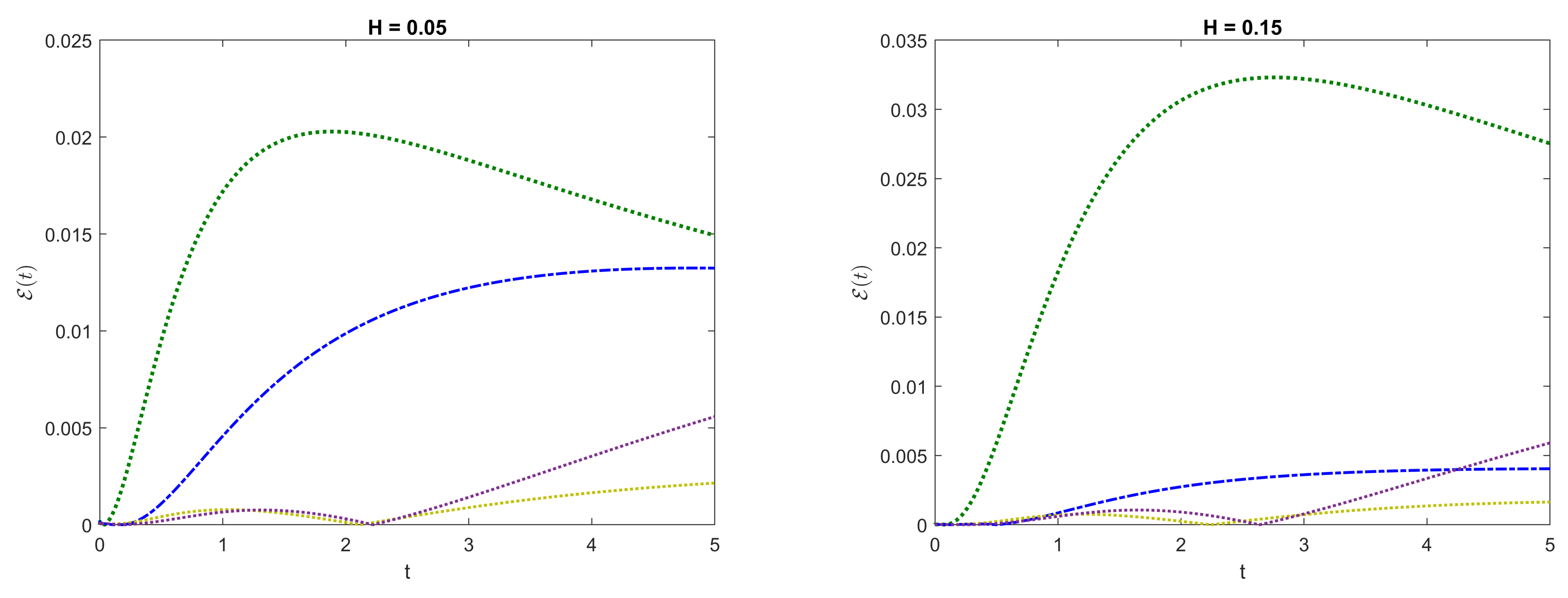
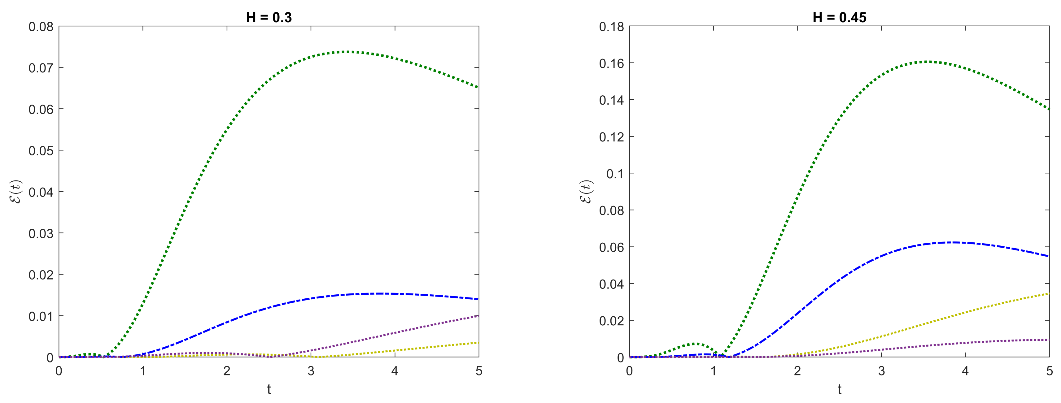
for the purpose of making comparisons on the solution of the fractional Riccati equation using different methods. Figure 1 shows the comparison of the solutions ( D α h ( 3 i / 2 , t ) ) by using the fractional Adams method, the GPadé method and the fourth-order global Padé approximation methods for ( m , n ) = ( 5 , 4 ) , ( 6 , 3 ) , ( 7 , 2 ) on different values of the Hurst parameter H.
Evidently, we can directly observe from Figure 1 and Figure 2 and Table 1 that fourth-order global Padé approximants h ( m , n ) ( a , t ) for ( m , n ) = ( 6 , 3 ) , ( 7 , 2 ) approximate the solution of the fractional Riccati equation in an extremely accurate manner. The key takeaway is that as compared to the GPadé method, the fourth-order global Padé approximants h ( m , n ) ( a , t ) for ( m , n ) = ( 6 , 3 ) , ( 7 , 2 ) remain well-behaved even when the Hurst parameter approaches 0.5.

6.2. Option Pricing

In this section, we utilize the methods we have developed throughout the paper to compute the option prices under the rough Heston model. The parameters used in the option pricing are:
ν = 0.4 ; ρ = 0.65 ; N = 100 ; ξ 0 ( t ) = 0.0225 t
where ν , ρ are from Equation (2), N is the number of time steps in fractional Adams method and ξ 0 ( t ) is the flat forward variance curve. We denote the average absolute error of the implied volatility as
E O ( T , H ) = 1 y i = 1 y | σ ( T , H , k i ) σ ( m , n ) ( T , H , k i ) |
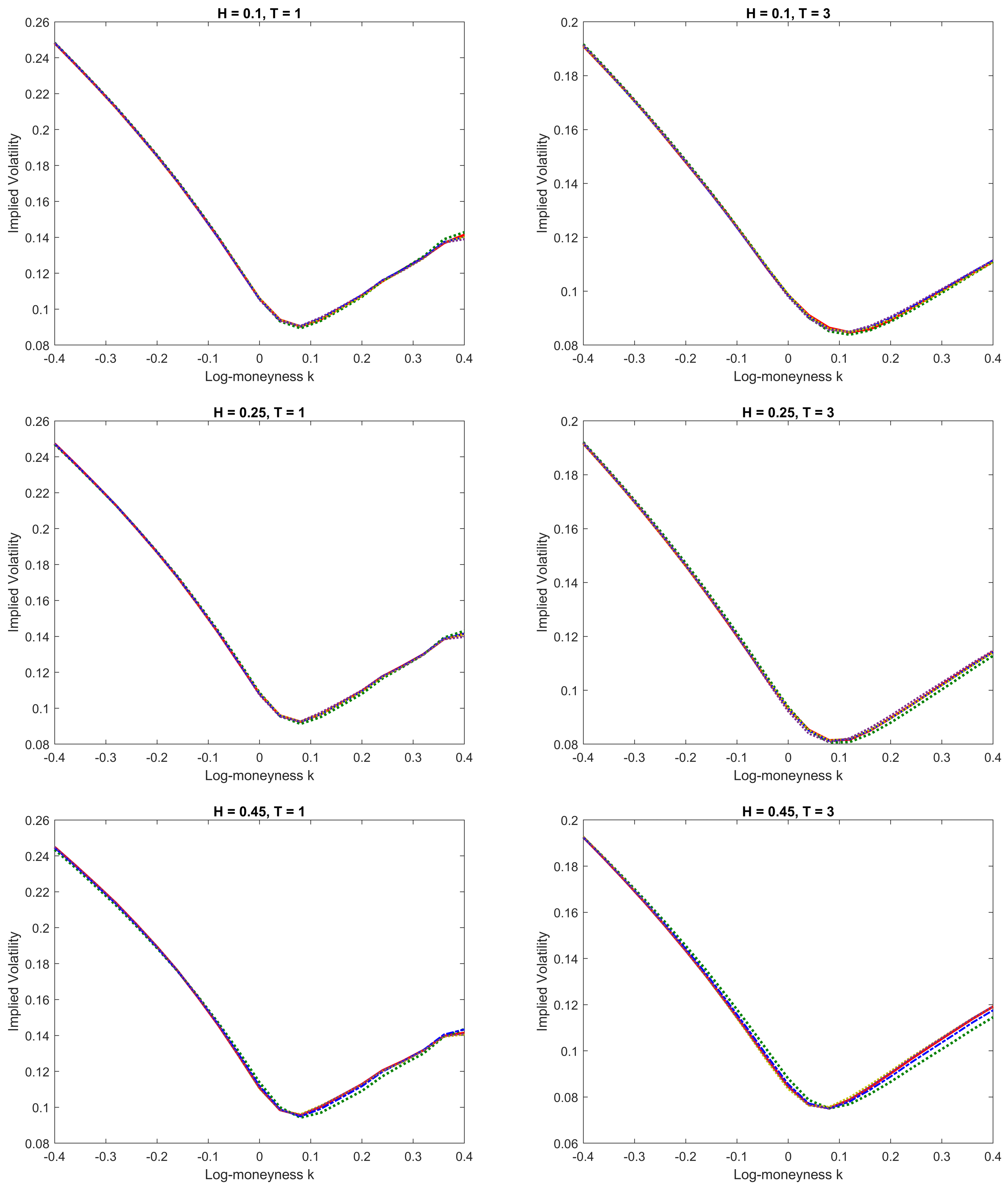
where k i [ 0.4 , 0.4 ] , y is the number of times implied volatility is sampled, σ ( T , H , k i ) is the implied volatility at log-moneyness k i obtained using the fractional Adams method and σ ( m , n ) ( T , H , k i ) is the implied volatility at log-moneyness k i being approximated using the GPadé method and fourth-order Padé approximants. From Table 2 and Figure 3, it is obvious that the fourth-order global Padé approximants performed better in all the circumstances that we evaluated. Notably, the use of the third-order global Padé approximant in computing option prices by [19] deteriorates the quality of the solution as the Hurst parameter H approaches 0.5 , whereas fourth-order global Padé approximants in computing option prices performed rather well and incurred lower errors. Fourth-order Padé approximants of h ( 6 , 3 ) ( a , t ) and h ( 7 , 2 ) ( a , t ) seem to provide the best overall performance as compared to h ( 5 , 4 ) ( a , t ) in computing the fractional Riccati equation’s solution.
It is important to realize that in the setting of option pricing under the rough Heston model, the application of the fractional Adams method to the fractional Riccati equation is undesirable in the real life calibration and computation due to its excessive computational cost needed (total time complexity of O ( n a N 2 ) where n a is the number of space steps for inversion of characteristic function (5), and N is the number of time steps for the fractional Adams method, (17)–(22)). For this reason, we have proposed and demonstrated the use of fourth-order global Padé approximants to approximate the fractional Riccati equation’s solution, and directly applied it to compute option prices under the rough Heston model with a total time complexity of just O ( n a ) . By considering efficiency, accuracy and robustness (Hurst parameter H), the proposed fourth-order global Padé approximation method is definitely preferable and superior in real life practice as compared to the existing work of the fractional Adams method and the third-order global Padé approximation [19].

7. Summary and Future Research

First off, we have provided an extensive literature review relevant to the fractional Riccati equation and rough Heston model. That included the general stochastic volatility models, rough volatility, the Hurst parameter and methods for obtaining option prices from the rough Heston model. This study heavily focuses on the numerical methods for computing the fractional Riccati equation’s solution. One of the key contributions from this paper is that the infinite series expansion of the fractional Riccati equation obtained using the Laplace–Adomian-decomposition method corresponds to the small time expansion of the fractional Riccati equation by [54] up to at least fifth order of the solution ( t 5 α ). Here we have implemented a fourth-order global Padé approximation method for the fractional Riccati equation; it includes the systems of equations in terms of the matrix to be solved in order to obtain the coefficients for fourth-order Padé approximants. The pointwise approximation errors on the global Padé approximation method for t 0 and t are also included, whereby it provides a sense of the number of terms (m and n) that we should pick from the small time and the large time series expansion solution of the fractional Riccati equation to solve for the coefficients of the fourth-order global Padé approximants. From the numerical computations of the fractional Riccati equation’s solution using different methods, we have found that indeed the fourth-order global Padé approximants performed the most consistently and robustly of any Hurst parameter on the solution of the fractional Riccati equation, unlike the third-order Padé approximant, for which it yields erroneous solutions as the Hurst parameters get closer to 0.5. Together with the application of the fractional Riccati equation, we computed option prices under different methods, and once again the fourth-order global Padé approximants performed the best as compared to the third-order global Padé approximant from the previous study by [19]. In addition to the accurate computation of the fractional Riccati equation’s solution, we note that the fourth-order global Padé approximation method possesses a time complexity of only O ( 1 ) (same as the third-order global Padé approximant) in solving the fractional Riccati equation as compared to the fractional Adams method that possesses a time complexity of O ( N 2 ) where N is the number of time steps. A key limitation of this global Padé approximation method is that while it guarantees pointwise convergence ( t 0 and t ) on the fractional Riccati equation’s solution, it does not provide any sense of convergence at elsewhere besides the two points.
Although we are able to reduce the errors of the fractional Riccati equation’s solution significantly as compared to the previous third-order Padé approximant, we wish to make three recommendations for future work: (1) consider higher order global Padé approximants such as fifth or sixth-order global Padé approximants to obtain for the fractional Riccati equation’s solution and subsequently apply them to the computation of option prices under the rough Heston model; (2) it would be interesting to see that this fourth order global Padé approximant is being applied to a general setting of the fractional Riccati equation, since they are applicable in many fields, such as physics, engineering and general mathematics; (3) while the third-order and fourth-order global Padé approximants have the same time complexity O ( 1 ) to compute for the fractional Riccati equation’s solution, we can further consider that by how much additional computational time is needed to switch from the third-order global Padé approximant to a fourth-order or perhaps fifth-order global Padé approximant given the advantage of accuracy and robustness in the Hurst parameter. Overall, it can be concluded that together with the small time and large time series expansions of the fractional Riccati equation’s solution, fourth-order global Padé approximants can be used to efficiently and accurately compute the option prices under varying Hurst parameter H.

Author Contributions

Conceptualization, S.W.J. and A.K.; methodology, S.W.J. and A.K.; software; S.W.J.; validation, S.W.J. and A.K.; formal analysis, S.W.J. and A.K.; investigation, S.W.J. and A.K.; resources, S.W.J. and A.K.; data curation, S.W.J.; writing—original draft preparation, S.W.J. and A.K.; writing—review and editing, A.K.; visualization, S.W.J.; supervision, A.K.; project administration, A.K.; funding acquisition, A.K. All authors have read and agreed to the published version of the manuscript.

Funding

The authors would like to acknowledge that this research is partially supported by Special Graduate Research Allowance (SGRA) with Vote number of 5540153.

Acknowledgments

The article was supported by the Fundamental Research Grant Scheme (FRGS) under the Ministry of Education with project number FRGS/1/2018/STG06/UPM/01/3.

Conflicts of Interest

The authors declare no conflict of interest.

Abbreviations

The following abbreviations are used in this manuscript:
fBmFractional Brownian motion
BSSHybrid Brownian semistationary method
LADMLaplace–Adomian-decomposition method
GPadéGatheral’s third-order Global Padé approximant

Appendix A. Riemann–Liouville Fractional Calculus

The Riemann–Liouville fractional integral and fractional derivative are presented in this Appendix A. More details of this section can be found in [64]. First, we define the Riemann–Liouville fractional integration as
I α f ( t ) = 1 Γ ( α ) 0 t f ( s ) ( t s ) 1 α d s
and the Riemann–Liouville fractional derivative as a
D α f ( t ) = d d t [ I 1 α f ( t ) ] = 1 Γ ( 1 α ) d d t 0 t f ( s ) ( t s ) α d s
where α ( 0 , 1 ] , t [ 0 , ) and Γ ( · ) is the standard gamma function. Moreover, Equations (A1) and (A2) revert back to the classical integration and differentiation when α = 1 .

Appendix B. The Laplace–Adomian-Decomposition Method on the Fractional Riccati Equation

In this Appendix B, we provide a step-by-step approach to obtaining a series expansion of the fractional Riccati equation’s solution using the Laplace–Adomian-decomposition method.
  • Step 1: We apply the Laplace transform to the both sides of the fractional Riccati Equation (6); then we can obtain the following equation:
    L { D α h ( a , t ) } = L { W } + R L { h ( a , t ) } + U L { h 2 ( a , t ) }
    From Equation (7), we can simplify the equation to
    s α L { h ( a , t ) } = W s + R L { h ( a , t ) } + U L { h 2 ( a , t ) }
    A further simplification gives us
    L { h ( a , t ) } = W s ( s α R ) + U s α R L { h 2 ( a , t ) }
  • Step 2: Let h ( t ) : = h ( a , t ) . The traditional Adomian decomposition method assumes that the solution is an infinite series:
    h ( t ) = n = 0 h n
    and the square of the solution h 2 is decomposed as
    f ( h ) : = h 2 ( t ) = n = 0 A n
    where A n : = A n ( h 0 , h 1 , , h n ) are the Adomian polynomials and can be computed using methods stated from [59,60]. The Adomian polynomials can be computed by the formula
    A n ( h 0 , h 1 , , h n ) = 1 n ! d n d λ n f ( i = 0 h i λ i ) λ = 0
    As for f ( h ) : = h 2 ( t ) , the first 12 Adomian polynomials A 0 , A 1 , , A 11 are computed by [31] as
    A 0 = h 0 2 , A 1 = 2 h 0 h 1 , A 2 = 2 h 0 h 2 + h 1 2 , A 3 = 2 h 0 h 3 + 2 h 1 h 2 , A 4 = 2 h 0 h 4 + 2 h 1 h 3 + h 2 2 , A 5 = 2 h 0 h 5 + 2 h 1 h 4 + 2 h 2 h 3 , A 6 = 2 h 0 h 6 + 2 h 1 h 4 + 2 h 2 h 4 + h 3 3 , A 7 = 2 h 0 h 7 + 2 h 1 h 6 + 2 h 2 h 5 + 2 h 3 h 4 , A 8 = 2 h 0 h 8 + 2 h 1 h 7 + 2 h 2 h 6 + 2 h 3 h 5 + h 4 2 , A 9 = 2 h 0 h 9 + 2 h 1 h 8 + 2 h 2 h 7 + 2 h 3 h 6 + 2 h 4 h 5 , A 10 = 2 h 0 h 10 + 2 h 1 h 9 + 2 h 2 h 8 + 2 h 3 h 7 + 2 h 4 h 6 + h 5 2 , A 11 = 2 h 0 h 11 + 2 h 1 h 10 + 2 h 2 h 9 + 2 h 3 h 8 + 2 h 4 h 7 + 2 h 5 h 6 .
  • Step 3: By substituting Equations (A6) and (A7) from Step 2 into Equation (A5), we obtain the following:
    L n = 0 h n = W s ( s α R ) + U s α R L n = 0 A n
    By matching both sides of Equation (A10) as in the usual Adomian decomposition method, we get
    L { h 0 } = W s ( s α R )
    L { h 1 } = U s α R L { A 0 }
    L { h 2 } = U s α R L { A 1 }
    L { h n } = U s α R L { A n 1 }
    Finally, we use the inverse Laplace transform on Equations (A11)–(A14) to obtain the terms h 0 , h 1 , . With the help of Lemma 1, we can obtain h 0 as
    h 0 = W t α E α , 1 + α ( R t α ) = W t α 1 Γ ( α + 1 ) + R t α Γ ( 2 α + 1 ) + ( R t α ) 2 Γ ( 3 α + 1 ) +
    Subsequently, A 0 is computed as follows:
    A 0 = h 0 2 = W 2 t 2 α [ 1 Γ ( α + 1 ) 2 + 2 R t α Γ ( α + 1 ) Γ ( 2 α + 1 ) + ( R t α ) 2 Γ ( 2 α + 1 ) 2 + 2 ( R t α ) 2 Γ ( α + 1 ) Γ ( 3 α + 1 ) + 2 ( R t α ) 3 Γ ( α + 1 ) Γ ( 4 α + 1 ) + 2 ( R t α ) 3 Γ ( 2 α + 1 ) Γ ( 3 α + 1 ) + 2 ( R t α ) 4 Γ ( α + 1 ) Γ ( 5 α + 1 ) + 2 ( R t α ) 4 Γ ( 3 α + 1 ) 2 + 2 ( R t α ) 4 Γ ( 2 α + 1 ) Γ ( 4 α + 1 ) + ]
    By performing an inverse Laplace transform on Equation (A12) and utilizing Lemma 2, we obtain h 1 as follows.
    h 1 = U W 2 [ Γ ( 2 α + 1 ) Γ ( α + 1 ) 2 t 3 α E α , 3 α + 1 ( R t α ) + 2 R Γ ( 3 α + 1 ) Γ ( α + 1 ) Γ ( 2 α + 1 ) t 4 α E α , 4 α + 1 ( R t α )   + R 2 Γ ( 4 α + 1 ) Γ ( 2 α + 1 ) 2 t 5 α E α , 5 α + 1 ( R t α ) + 2 R 2 Γ ( 4 α + 1 ) Γ ( α + 1 ) Γ ( 3 α + 1 ) t 5 α E α , 5 α + 1 ( R t α )   + 2 R 3 Γ ( 5 α + 1 ) Γ ( α + 1 ) Γ ( 4 α + 1 ) t 6 α E α , 6 α + 1 ( R t α ) + 2 R 3 Γ ( 5 α + 1 ) Γ ( 2 α + 1 ) Γ ( 3 α + 1 ) t 6 α E α , 6 α + 1 ( R t α )   + 2 R 4 Γ ( 6 α + 1 ) Γ ( α + 1 ) Γ ( 5 α + 1 ) t 7 α E α , 7 α + 1 ( R t α ) + R 4 Γ ( 6 α + 1 ) Γ ( 3 α + 1 ) 2 t 7 α E α , 7 α + 1 ( R t α )   + 2 R 4 Γ ( 6 α + 1 ) Γ ( 2 α + 1 ) Γ ( 4 α + 1 ) t 7 α E α , 7 α + 1 ( R t α ) + ] = U W 2 [ Γ ( 2 α + 1 ) t 3 α Γ ( α + 1 ) 2 Γ ( 3 α + 1 ) + R Γ ( 2 α + 1 ) t 4 α Γ ( α + 1 ) 2 Γ ( 4 α + 1 ) + 2 R Γ ( 3 α + 1 ) t 4 α Γ ( α + 1 ) Γ ( 2 α + 1 ) Γ ( 4 α + 1 )   + R 2 Γ ( 4 α + 1 ) t 5 α Γ ( 2 α + 1 ) 2 Γ ( 5 α + 1 ) + 2 R 2 Γ ( 4 α + 1 ) t 5 α Γ ( α + 1 ) Γ ( 3 α + 1 ) Γ ( 5 α + 1 ) + R 2 Γ ( 2 α + 1 ) t 5 α Γ ( α + 1 ) 2 Γ ( 5 α + 1 )   + 2 R 2 Γ ( 3 α + 1 ) t 5 α Γ ( α + 1 ) Γ ( 2 α + 1 ) Γ ( 5 α + 1 ) + ]
    We repeat the process by letting A 1 = 2 h 0 h 1 , and then performing an inverse Laplace transform on L { h 2 } in Equation (A13). Similarly, we use Lemma 2 to obtain h 2 as
    h 2 = 2 U 2 W 3 [ Γ ( 2 α + 1 ) Γ ( 4 α + 1 ) t 5 α Γ ( α + 1 ) 3 Γ ( 3 α + 1 ) Γ ( 5 α + 1 ) + R Γ ( 2 α + 1 ) Γ ( 4 α + 1 ) t 6 α Γ ( α + 1 ) 3 Γ ( 3 α + 1 ) Γ ( 6 α + 1 )   + R Γ ( 2 α + 1 ) Γ ( 5 α + 1 ) t 6 α Γ ( α + 1 ) 3 Γ ( 4 α + 1 ) Γ ( 6 α + 1 ) + R Γ ( 5 α + 1 ) t 6 α Γ ( α + 1 ) 3 Γ ( 3 α + 1 ) Γ ( 6 α + 1 )   + 2 R Γ ( 3 α + 1 ) Γ ( 5 α + 1 ) t 6 α Γ ( α + 1 ) 2 Γ ( 2 α + 1 ) Γ ( 4 α + 1 ) Γ ( 6 α + 1 ) + ]
    Repeat the process to obtain h 3 , h 4 , , h n , and finally we have the following expansion:
    h ( a , t ) = h 0 + h 1 + h 2 + = W t α Γ ( α + 1 ) + W R t 2 α Γ ( 2 α + 1 ) + W R 2 t 3 α Γ ( 3 α + 1 ) + U W 2 Γ ( 2 α + 1 ) t 3 α Γ ( α + 1 ) 2 Γ ( 3 α + 1 )   + W R 3 t 4 α Γ ( 4 α + 1 ) + U R W 2 Γ ( 2 α + 1 ) t 4 α Γ ( α + 1 ) 2 Γ ( 4 α + 1 ) + 2 U R W 2 Γ ( 3 α + 1 ) t 4 α Γ ( α + 1 ) Γ ( 2 α + 1 ) Γ ( 4 α + 1 )   + W R 4 t 5 α Γ ( 5 α + 1 ) + U W 2 R 2 Γ ( 4 α + 1 ) t 5 α Γ ( 2 α + 1 ) 2 Γ ( 5 α + 1 ) + 2 U W 2 R 2 Γ ( 4 α + 1 ) t 5 α Γ ( α + 1 ) Γ ( 3 α + 1 ) Γ ( 5 α + 1 )   + U W 2 R 2 Γ ( 2 α + 1 ) t 5 α Γ ( α + 1 ) 2 Γ ( 5 α + 1 ) + 2 U W 2 R 2 Γ ( 3 α + 1 ) t 5 α Γ ( α + 1 ) Γ ( 2 α + 1 ) Γ ( 5 α + 1 )   + 2 U 2 W 3 Γ ( 2 α + 1 ) Γ ( 4 α + 1 ) t 5 α Γ ( α + 1 ) 3 Γ ( 3 α + 1 ) Γ ( 5 α + 1 ) +
  • Step 4: For our purpose of study, from Equation (4), we substitute the following U = 1 2 ν 2 , R = i ρ a ν and W = 1 2 a ( a + i ) to Equation (A19). Let the series expansion of h ( a , t ) to be in the form of
    h ( a , t ) = Λ 1 t α + Λ 2 t 2 α + Λ 3 t 3 α + Λ 4 t 4 α + Λ 5 t 5 α +
    Finally, the first five coefficients are
    Λ 1 = 1 2 a ( a + i ) Γ ( α + 1 ) Λ 2 = ( 1 2 a ( a + i ) ) ( i ρ a ν ) Γ ( 2 α + 1 ) Λ 3 = ( 1 2 a ( a + i ) ) ( i ρ a ν ) 2 Γ ( 3 α + 1 ) + 1 2 ν 2 ( 1 2 a ( a + i ) ) 2 Γ ( 2 α + 1 ) Γ ( α + 1 ) 2 Γ ( 3 α + 1 ) Λ 4 = ( 1 2 a ( a + i ) ) ( i ρ a ν ) 3 Γ ( 4 α + 1 ) + 1 2 i ρ a ν 3 ( 1 2 a ( a + i ) ) 2 Γ ( 2 α + 1 ) Γ ( α + 1 ) 2 Γ ( 4 α + 1 )   + i ρ a ν 3 ( 1 2 a ( a + i ) ) 2 Γ ( 3 α + 1 ) Γ ( α + 1 ) Γ ( 2 α + 1 ) Γ ( 4 α + 1 ) Λ 5 = ( 1 2 a ( a + i ) ) ( i ρ a ν ) 4 Γ ( 5 α + 1 ) + 1 2 ν 2 ( 1 2 a ( a + i ) ) 2 ( i ρ a ν ) 2 Γ ( 4 α + 1 ) Γ ( 2 α + 1 ) 2 Γ ( 5 α + 1 )   + ν 2 ( 1 2 a ( a + i ) ) 2 ( i ρ a ν ) 2 Γ ( 4 α + 1 ) Γ ( α + 1 ) Γ ( 3 α + 1 ) Γ ( 5 α + 1 ) + 1 2 ν 2 ( 1 2 a ( a + i ) ) 2 ( i ρ a ν ) 2 Γ ( 2 α + 1 ) Γ ( α + 1 ) 2 Γ ( 5 α + 1 )   + ν 2 ( 1 2 a ( a + i ) ) 2 ( i ρ a ν ) 2 Γ ( 3 α + 1 ) Γ ( α + 1 ) Γ ( 2 α + 1 ) Γ ( 5 α + 1 ) + 1 2 ν 4 ( 1 2 a ( a + i ) ) 3 Γ ( 2 α + 1 ) Γ ( 4 α + 1 ) Γ ( α + 1 ) 3 Γ ( 3 α + 1 ) Γ ( 5 α + 1 )

References

  1. Black, F.; Scholes, M. The pricing of options and corporate liabilities. J. Political Econ. 1973, 81, 637–654. [Google Scholar] [CrossRef] [Green Version]
  2. Merton, R.C. Option pricing when underlying stock returns are discontinuous. J. Financ. Econ. 1976, 3, 125–144. [Google Scholar] [CrossRef] [Green Version]
  3. Hull, J.; White, A. The pricing of options on assets with stochastic volatilities. J. Financ. 1987, 42, 281–300. [Google Scholar] [CrossRef]
  4. Heston, S.L. A closed-form solution for options with stochastic volatility with applications to bond and currency options. Rev. Financ. Stud. 1993, 6, 327–343. [Google Scholar] [CrossRef] [Green Version]
  5. Renault, E.; Touzi, N. Option hedging and implied volatilities in a stochastic volatility model 1. Math. Financ. 1996, 6, 279–302. [Google Scholar] [CrossRef]
  6. Lee, R.W. Implied volatility: Statics, dynamics, and probabilistic interpretation. In Recent Advances in Applied Probability; Springer: Berlin, Germany, 2005; pp. 241–268. [Google Scholar]
  7. Lewis, A.L. Option Valuation under Stochastic Volatility II; Finance Press: Newport Beach, CA, USA, 2009. [Google Scholar]
  8. Medvedev, A.; Scaillet, O. Approximation and calibration of short-term implied volatilities under jump-diffusion stochastic volatility. Rev. Financ. Stud. 2007, 20, 427–459. [Google Scholar] [CrossRef] [Green Version]
  9. Bates, D.S. Jumps and stochastic volatility: Exchange rate processes implicit in deutsche mark options. Rev. Financ. Stud. 1996, 9, 69–107. [Google Scholar] [CrossRef]
  10. Mandelbrot, B.B.; Van Ness, J.W. Fractional Brownian motions, fractional noises and applications. SIAM Rev. 1968, 10, 422–437. [Google Scholar] [CrossRef]
  11. Comte, F.; Renault, E. Long memory in continuous-time stochastic volatility models. Math. Financ. 1998, 8, 291–323. [Google Scholar] [CrossRef]
  12. Cheridito, P. Mixed fractional Brownian motion. Bernoulli 2001, 7, 913–934. [Google Scholar] [CrossRef]
  13. Gatheral, J.; Jaisson, T.; Rosenbaum, M. Volatility is rough. Quant. Financ. 2018, 18, 933–949. [Google Scholar] [CrossRef]
  14. Fukasawa, M. Asymptotic analysis for stochastic volatility: Martingale expansion. Financ. Stoch. 2011, 15, 635–654. [Google Scholar] [CrossRef] [Green Version]
  15. Alòs, E.; León, J.A.; Vives, J. On the short-time behavior of the implied volatility for jump-diffusion models with stochastic volatility. Financ. Stoch. 2007, 11, 571–589. [Google Scholar] [CrossRef] [Green Version]
  16. Bayer, C.; Friz, P.; Gatheral, J. Pricing under rough volatility. Quant. Financ. 2016, 16, 887–904. [Google Scholar] [CrossRef]
  17. El Euch, O.; Rosenbaum, M. The characteristic function of rough Heston models. Math. Financ. 2019, 29, 3–38. [Google Scholar] [CrossRef] [Green Version]
  18. El Euch, O.; Fukasawa, M.; Rosenbaum, M. The microstructural foundations of leverage effect and rough volatility. Financ. Stoch. 2018, 22, 241–280. [Google Scholar] [CrossRef] [Green Version]
  19. Gatheral, J.; Radoicic, R. Rational approximation of the rough Heston solution. Int. J. Theor. Appl. Financ. 2019, 22, 1950010. [Google Scholar] [CrossRef]
  20. Bennedsen, M.; Lunde, A.; Pakkanen, M.S. Hybrid scheme for Brownian semistationary processes. Financ. Stoch. 2017, 21, 931–965. [Google Scholar] [CrossRef] [Green Version]
  21. McCrickerd, R.; Pakkanen, M.S. Turbocharging Monte Carlo pricing for the rough Bergomi model. Quant. Financ. 2018, 18, 1877–1886. [Google Scholar] [CrossRef] [Green Version]
  22. Abi Jaber, E.; El Euch, O. Multifactor Approximation of Rough Volatility Models. SIAM J. Financ. Math. 2019, 10, 309–349. [Google Scholar] [CrossRef] [Green Version]
  23. Abi Jaber, E. Lifting the Heston model. Quant. Financ. 2019, 19, 1995–2013. [Google Scholar] [CrossRef]
  24. El Euch, O.; Gatheral, J.; Rosenbaum, M. Roughening Heston. 2018. Available online: https://ssrn.com/abstract=3116887 (accessed on 25 March 2019).
  25. Callegaro, G.; Grasselli, M.; Pages, G. Rough but not so tough: Fast hybrid schemes for fractional Riccati equations. arXiv 2018, arXiv:1805.12587. [Google Scholar]
  26. Odibat, Z.; Momani, S. Application of variational iteration method to nonlinear differential equations of fractional order. Int. J. Nonlinear Sci. Numer. Simul. 2006, 7, 27–34. [Google Scholar] [CrossRef]
  27. Momani, S.; Shawagfeh, N. Decomposition method for solving fractional Riccati differential equations. Appl. Math. Comput. 2006, 182, 1083–1092. [Google Scholar] [CrossRef]
  28. Cang, J.; Tan, Y.; Xu, H.; Liao, S.J. Series solutions of non-linear Riccati differential equations with fractional order. Chaos Solitons Fractals 2009, 40, 1–9. [Google Scholar] [CrossRef]
  29. Odibat, Z.; Momani, S. Modified homotopy perturbation method: Application to quadratic Riccati differential equation of fractional order. Chaos Solitons Fractals 2008, 36, 167–174. [Google Scholar] [CrossRef]
  30. Khan, N.A.; Ara, A.; Khan, N.A. Fractional-order Riccati differential equation: Analytical approximation and numerical results. Adv. Differ. Equ. 2013, 185. [Google Scholar] [CrossRef] [Green Version]
  31. Tsai, P.-Y.; Chen, C.-K. An approximate analytic solution of the nonlinear Riccati differential equation. J. Frankl. Inst. 2010, 347, 1850–1862. [Google Scholar] [CrossRef]
  32. Jafari, H.; Tajadodi, H.; Matikolai, S.H. Homotopy perturbation pade technique for solving fractional Riccati differential equations. Int. J. Nonlinear Sci. Numer. Simul. 2010, 11, 271–276. [Google Scholar] [CrossRef]
  33. Raja, M.A.Z.; Khan, J.A.; Qureshi, I.M. A new stochastic approach for solution of Riccati differential equation of fractional order. Ann. Math. Artif. Intell. 2010, 60, 229–250. [Google Scholar] [CrossRef]
  34. Merino, R.; Vives, J. A generic decomposition formula for pricing vanilla options under stochastic volatility models. Int. J. Stoch. Anal. 2015, 3, 125–144. [Google Scholar] [CrossRef]
  35. Alòs, E. A decomposition formula for option prices in the Heston model and applications to option pricing approximation. Quant. Financ. 2012, 20, 13–27. [Google Scholar] [CrossRef]
  36. Alós, E.; Yang, Y. A Closed-Form Option Pricing Approximation Formula for a Fractional Heston Model. Economics Working Papers. 2014. Available online: https://econ-papers.upf.edu/papers/1446.pdf (accessed on 1 September 2020).
  37. Diethelm, K.; Ford, N.J.; Freed, A.D. Detailed error analysis for a fractional Adams method. Numer. Algorithms 2004, 36, 31–52. [Google Scholar] [CrossRef] [Green Version]
  38. Carr, P.; Madan, D. Option valuation using the fast Fourier transform. J. Comput. Financ. 1999, 2, 61–73. [Google Scholar] [CrossRef] [Green Version]
  39. Lewis, A.L. A Simple Option Formula for General Jump-Diffusion and Other Exponential Lévy Processes. 2001. Available online: https://ssrn.com/abstract=282110 (accessed on 15 February 2020).
  40. Thompson, I.J. Coupled reaction channels calculations in nuclear physics. Comput. Phys. Rep. 1988, 7, 167–212. [Google Scholar] [CrossRef]
  41. Rakityansky, S.; Sofianos, S.; Elander, N. Pade approximation of the S-matrix as a way of locating quantum resonances and bound states. J. Phys. A Math. Theor. 2007, 40, 14857. [Google Scholar] [CrossRef] [Green Version]
  42. Lanti, E.; Dominski, J.; Brunner, S.; McMillan, B.; Villard, L. Padé Approximation of the adiabatic electron contribution to the gyrokinetic quasi-neutrality equation in the ORB5 code. In Proceedings of the Joint Varenna-Lausanne International Workshop on the Theory of Fusion Plasmas, Varenna, Italy, 29 August–2 September 2016; IOP Publishing: Bristol, UK, 2016; Volume 775, p. 012006. [Google Scholar]
  43. Baker, G.A.; Graves-Morris, P. Padé Approximants; Cambridge University Press: Cambridge, UK, 1996; Volume 59. [Google Scholar]
  44. Lubinsky, D.S. Rogers-Ramanujan and the Baker-Gammel-Wills (padé) conjecture. Ann. Math. 2003, 157, 847–889. [Google Scholar] [CrossRef]
  45. Lubinsky, D.S. Reflections on the Baker–Gammel–Wills (Padé) Conjecture. In Analytic Number Theory, Approximation Theory, and Special Functions; Springer: Berlin, Germany, 2014; pp. 561–571. [Google Scholar]
  46. Jeng, S.W.; Kilicman, A. Fractional Riccati Equation and Its Applications to Rough Heston Model Using Numerical Methods. Symmetry 2020, 12, 959. [Google Scholar] [CrossRef]
  47. Winitzki, S. Uniform approximations for transcendental functions. In International Conference on Computational Science and Its Applications; Springer: Berlin, Germany, 2003; pp. 780–789. [Google Scholar]
  48. Abassy, T.A.; El-Tawil, M.A.; El-Zoheiry, H. Exact solutions of some nonlinear partial differential equations using the variational iteration method linked with laplace transforms and the padé technique. Comput. Math. Appl. 2007, 54, 940–954. [Google Scholar] [CrossRef] [Green Version]
  49. Dehghan, M.; Hamidi, A.; Shakourifar, M. The solution of coupled Burgers’ equations using Adomian–Pade technique. Appl. Math. Comput. 2007, 189, 1034–1047. [Google Scholar] [CrossRef]
  50. Atkinson, C.; Osseiran, A. Rational solutions for the time-fractional diffusion equation. SIAM J. Appl. Math. 2011, 71, 92–106. [Google Scholar] [CrossRef]
  51. Zeng, C.; Chen, Y.Q. Global Padé approximations of the generalized Mittag-Leffler function and its inverse. Fract. Calc. Appl. Anal. 2015, 18, 1492–1506. [Google Scholar] [CrossRef] [Green Version]
  52. Starovoitov, A.P.; Starovoitova, N.A. Padé approximants of the Mittag-Leffler functions. Sb. Math. 2007, 198, 1011. [Google Scholar] [CrossRef]
  53. Sarumi, I.O.; Furati, K.M.; Khaliq, A.Q. Highly Accurate Global Padé Approximations of Generalized Mittag–Leffler Function and Its Inverse. J. Sci. Comput. 2020, 82, 46. [Google Scholar] [CrossRef] [Green Version]
  54. Alos, E.; Gatheral, J.; Radoičić, R. Exponentiation of conditional expectations under stochastic volatility. Quant. Financ. 2020, 20, 13–27. [Google Scholar] [CrossRef]
  55. El Euch, O.; Rosenbaum, M. Perfect hedging in rough Heston models. Ann. Appl. Probab. 2018, 28, 3813–3856. [Google Scholar] [CrossRef] [Green Version]
  56. Gatheral, J. The Volatility Surface: A Practitioner’s Guide; John Wiley & Sons: Hoboken, NJ, USA, 2011; Volume 357. [Google Scholar]
  57. Podlubny, I. The Laplace transform method for linear differential equations of the fractional order. arXiv 1997, arXiv:funct-an/9710005. [Google Scholar]
  58. Schiff, J.L. The Laplace Transform: Theory and Applications; Springer Science & Business Media: New York, NY, USA, 2013. [Google Scholar]
  59. Biazar, J.; Pourabd, M. A Maple program for computing Adomian polynomials. Int. Math. Forum 2006, 1, 1919–1924. [Google Scholar] [CrossRef]
  60. Biazar, J.; Shaof, S. A simple algorithm for calculating Adomian polynomials. Int. J. Contemp. Math. Sci. 2007, 2, 975–982. [Google Scholar] [CrossRef] [Green Version]
  61. Diethelm, K.; Freed, A.D. The FracPECE Subroutine for the Numerical Solution of Differential Equations of Fractional Order. Semantic Scholar. 1999. Available online: https://static.aminer.org/pdf/PDF/000/243/047/numerical_approaches_to_the_solution_of_some_fractional_differential_equations.pdf (accessed on 15 May 2020).
  62. Diethelm, K.; Freed, A.D. On the solution of nonlinear fractional-order differential equations used in the modeling of viscoplasticity. In Scientific Computing in Chemical Engineering II; Springer: Berlin/Heidelberg, Germany, 1999; pp. 217–224. [Google Scholar]
  63. Diethelm, K.; Ford, N.J.; Freed, A.D.; Luchko, Y. Algorithms for the fractional calculus: A selection of numerical methods. Comput. Methods Appl. Mech. Eng. 2005, 194, 743–773. [Google Scholar] [CrossRef] [Green Version]
  64. Dumitru, B.; Kai, D.; Enrico, S. Fractional Calculus: Models and Numerical Methods; World Scientific: Singapore, 2012; Volume 3. [Google Scholar]
  65. Li, C.; Tao, C. On the fractional Adams method. Comput. Math. Appl. 2009, 58, 1573–1588. [Google Scholar] [CrossRef] [Green Version]
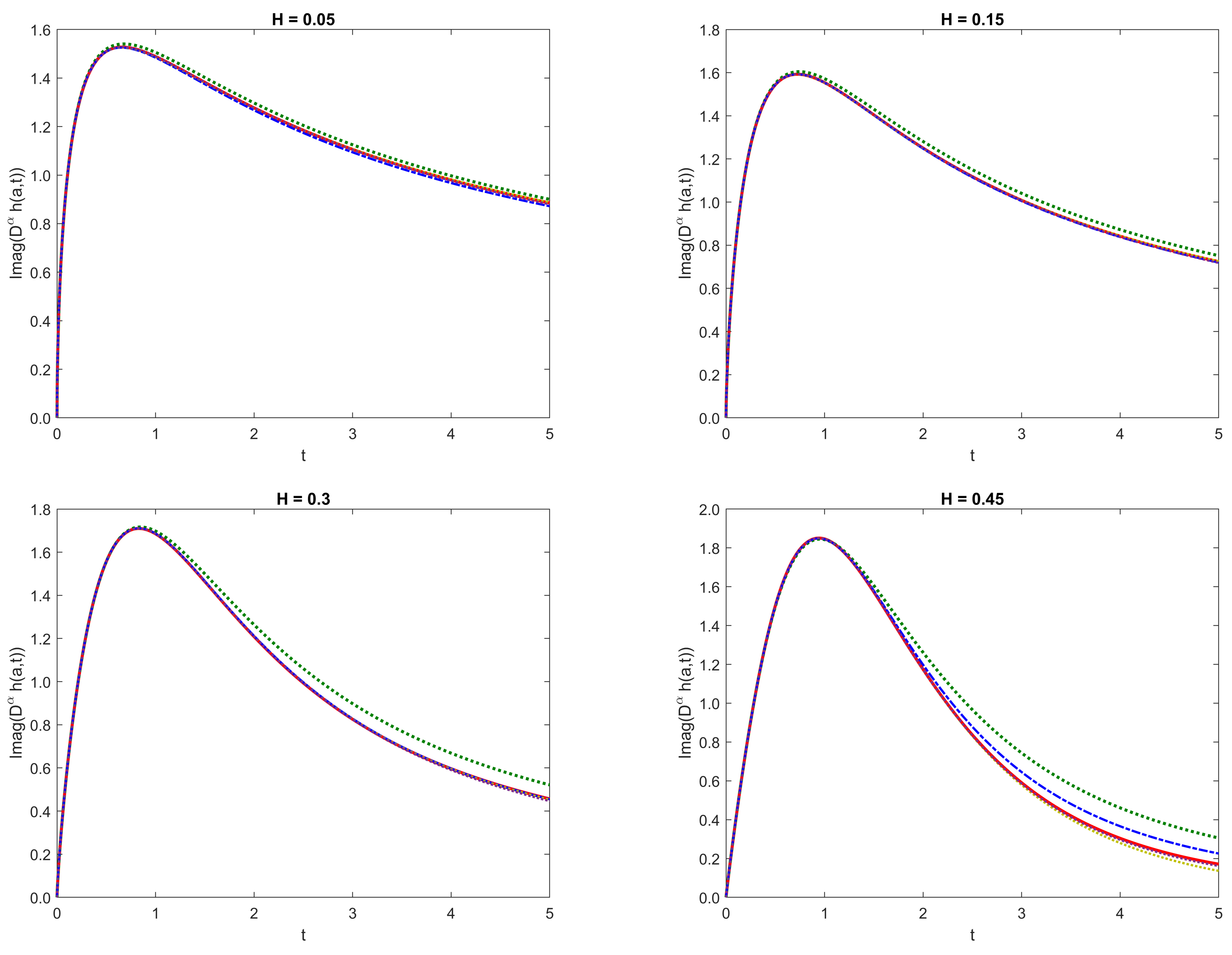
Figure 1. Comparison of solutions ( D α h ( 3 i / 2 , t ) ) using the fractional Adams method (solid red line) [61], the third-order GPadé approximant (dotted dark green) [19] and the fourth-order h ( m , n ) ( a , t ) for ( m , n ) = ( 5 , 4 ) , ( 6 , 3 ) , ( 7 , 2 ) (dashed-dotted dark blue, dotted mustard and dotted dark purple lines respectively) and a = 3 i / 2 .
Mathematics 08 01968 g001
Figure 2. Plots of E ( t ) for third-order GPadé approximant (dotted dark green) [19] and fourth-order h ( m , n ) ( a , t ) for ( m , n ) = ( 5 , 4 ) , ( 6 , 3 ) , ( 7 , 2 ) (dashed-dotted dark blue, dotted mustard and dotted dark purple lines respectively) and a = 3 i / 2 .
Mathematics 08 01968 g002aMathematics 08 01968 g002b
Figure 3. Implied volatility plots using the fractional Adams method (solid red line), the third-order GPadé approximant (dotted dark green) [19] and the fourth-order h ( m , n ) ( a , t ) for ( m , n ) = ( 5 , 4 ) , ( 6 , 3 ) , ( 7 , 2 ) (dashed-dotted dark blue, dotted mustard and dotted dark purple lines respectively).
Mathematics 08 01968 g003
Table 1. Maximum absolute errors for different approximants.
GPadé [19] h ( 5 , 4 ) ( a , t ) h ( 6 , 3 ) ( a , t ) h ( 7 , 2 ) ( a , t )
D ( 0.05 ) 0.02830.01320.00220.0056
D ( 0.10 ) 0.02520.00800.00190.0057
D ( 0.15 ) 0.03230.00400.00160.0059
D ( 0.20 ) 0.04230.00080.00130.0065
D ( 0.30 ) 0.07370.01530.00350.0100
D ( 0.45 ) 0.16050.06230.03460.0094
D ( 0.49 ) 0.19460.08380.04690.0155
Table 2. Average absolute error of the implied volatility in terms of 10 3 .
GPadé [19] h ( 5 , 4 ) ( a , t ) h ( 6 , 3 ) ( a , t ) h ( 7 , 2 ) ( a , t )
E O ( 1 , 0.10 ) 0.62400.25680.24000.4816
E O ( 1 , 0.25 ) 0.76630.07120.11790.3834
E O ( 1 , 0.45 ) 1.79170.63080.26510.1009
E O ( 3 , 0.10 ) 0.58020.28740.22320.5417
E O ( 3 , 0.25 ) 1.07780.12570.11240.5995
E O ( 3 , 0.45 ) 2.64520.94040.53560.1566
Publisher’s Note: MDPI stays neutral with regard to jurisdictional claims in published maps and institutional affiliations.