Perspectives on Adversarial Classification

Abstract

Adversarial classification (AC) is a major subfield within the increasingly important domain of adversarial machine learning (AML). So far, most approaches to AC have followed a classical game-theoretic framework. This requires unrealistic common knowledge conditions untenable in the security settings typical of the AML realm. After reviewing such approaches, we present alternative perspectives on AC based on adversarial risk analysis.

1. Introduction

Classification is a major research area with important applications in security and cybersecurity, including fraud detection [1]: phishing detection [2], terrorism [3] or cargo screening [4]. An increasing number of processes are being automated through classification algorithms; it is essential that these are robust to trust key operations based on their output. State-of-the-art classifiers perform extraordinarily well on standard data, but they have been shown to be vulnerable to adversarial examples, that is, data instances targeted at fooling the underlying algorithms. Ref. [5] provides an excellent introduction from a policy perspective, pointing out the potentially enormous security impacts that such attacks may have over systems for filter content, predictive policing or autonomous driving, to name but a few.

Most research in classification has focused on obtaining more accurate algorithms, largely ignoring the eventual presence of adversaries who actively manipulate data to fool the classifier in pursue of a benefit. Consider spam detection: as classification algorithms are incorporated to such task, spammers learn how to evade them. Thus, rather than sending their spam messages in standard language, they slightly modify spam words (frequent in spam messages but not so much in legitimate ones), misspell them or change them with synonyms; or they add good words (frequent in legitimate emails but not in spam ones) to fool the detection system.

Consequently, classification algorithms in critical AI-based systems must be robust against adversarial data manipulations. To this end, they have to take into account possible modifications of input data due to adversaries. The subfield of classification that seeks for algorithms with robust behaviour against adversarial perturbations is known as adversarial classification (AC) and was pioneered by [6]. Stemming from their work, the prevailing paradigm when modelling the confrontation between classification systems and adversaries has been game theory, see recent reviews [7,8]. This entails well-known common knowledge hypothesis [9,10] according to which agents share information about their beliefs and preferences. From a fundamental point of view, this is not sustainable in application areas such as security or cybersecurity, as participants try to hide and conceal information.

After reviewing key developments in game-theoretic approaches to AC in Section 2 and Section 3, we cover novel techniques based on adversarial risk analysis (ARA) in Section 4 and Section 5 [11]. Their key advantage is that they do not assume strong common knowledge hypothesis concerning belief and preference sharing, as with standard game theoretic approaches to AML. In this, we unify, expand and improve upon earlier work in [12,13]. Our focus will be on binary classification problems in face only of exploratory attacks, defined to have influence over operational data but not over training ones. In addition, we restrict our attention to attacks affecting only malicious instances, denominated integrity-violation attacks, the usual context in most security scenarios. We assume that the attacker will, at least, try to modify every malicious instance before the classifier actually observes it. Moreover, attacks will be assumed to be deterministic, in that we can predict for sure the results of their application over a given instance. Refs. [14,15] provide taxonomies of attacks against classifiers. We first consider approaches in which learning about the adversary is performed in the operational phase, studying how to robustify generative and discriminative classifiers against attacks. In certain applications, these could be very demanding from a computational perspective; for those cases, we present in Section 5 an approach in which adversarial aspects are incorporated in the training phase. Section 6 illustrates the proposed framework with spam detection and image processing examples.

2. Attacking Classification Algorithms

2.1. Binary Classification Algorithms

In binary classification settings, an agent that we call classifier (C, she) may receive instances belonging to one of two possible classes denoted, in our context, as malicious ($y=y_1$) or innocent ($y=y_2$). Instances have features $x\in {\mathbb{R}}^d$ whose distribution informs about their class y. Most classification approaches can be typically broken down in two separate stages, the training and operational phases [16].

The first one is used to learn the distribution $p_C\left(y\right|x)$, modelling the classifier’s beliefs about the instance class y given its features x. Frequently, a distinction is introduced between generative and discriminative models. In the first case, models $p_C\left(x\right|y)$ and $p_C\left(y\right)$ are learnt from training data; based on them, $p_C\left(y\right|x)$ is deduced through Bayes formula. Typical examples include Naive Bayes [17] and (conditional) variational autoencoders [18]. In discriminative cases, $p_C\left(y\right|x)$ is directly learnt from data. Within these, an important group of methods uses a parameterised function $f_{\beta }:{\mathbb{R}}^d\to {\mathbb{R}}^2$ so that the prediction is given through $p_C\left(y\right|x,\beta )=\mathrm{softmax}\left(f_{\beta }\left(x\right)\right)\left[y\right]$: when $f_{\beta }\left(x\right)={\beta }^{\prime }x$, we recover the logistic regression model [19]; if $f_{\beta }$ is a sequence of linear transformations alternating certain nonlinear activation functions, we obtain a feed-forward neural network [16]. Learning depends then on the underlying methodology adopted.

• In frequentist approaches, training data $D$ is typically used to construct a (possibly regularised) maximum likelihood estimate $\widehat{\beta }$, and $p_C\left(y\right|\widehat{\beta },x)$ is employed for classification. Parametric differentiable models are amenable to training with stochastic gradient descent (SGD) [20] using a minibatch of samples at each iteration. This facilitates, e.g., training deep neural networks with large amounts of high-dimensional data as with images or text data [21].
• In Bayesian approaches, a prior $p_C\left(\beta \right)$ is used to compute the posterior $p_C\left(\beta \right|D)$, given the data $D$, and the predictive distribution

  $$p_C\left(y\right|x,D)=\int p_C\left(y\right|\beta ,x)p_C\left(\beta \right|D)d\beta$$

  (1)

  is used to classify. Given current technology, in complex environments we are sometimes only able to approximate the posterior mode $\widehat{\beta }$, then using $p_C\left(y\right|\widehat{\beta },x)$.

In any case, and whatever the learning approach adopted, we shall use the notation $p_C\left(y\right|x)$.

The second stage is operational. The agent makes class assignment decisions based on $p_C\left(y\right|x)$. This may be formulated through the influence diagram (ID) [22] in Figure 1. In it, square nodes describe decisions; circle nodes, uncertainties; hexagonal nodes refer to the associated utilities. Arcs pointing to decision nodes are dashed and represent information available when the corresponding decisions are made. Arcs pointing to chance and value nodes suggest conditional dependence.

The classifier guess $y_c$ for an observed instance x provides her with a utility $u_C(y_c,y_i)$ when the actual class is $y_i$ and she aims at maximising expected utility through

$$arg\underset{y_c}{max}\sum _{i=1}^2{u}_C(y_c,y_i)p_C\left(y_i\right|x).$$

(2)

An important example of utility functions is the 0-1 utility: $u_C(y_c,y_i)=\mathbb{I}(y_c=y_i)$, where $\mathbb{I}$ is the indicator function. This leads to deciding based on maximising the predictive probability of correct classification

$$arg\underset{y_c}{max}\sum _{i=1}^2\mathbb{I}(y_c=y_i)p_C\left(y_i\right|x)=arg\underset{y_c}{max}{p}_C\left(y_c\right|x).$$

(3)

In general, the utility is characterised as a $2\times 2$ matrix, whose $ij$-th entry represents the utility that the classifier receives for classifying an instance of true label j as of being of class i. This essentially balances the relative importance of false positives and negatives. Consider the case of autonomous driving systems. In it, proper classification of identified objects is of major importance. Misclassification errors increase the likelihood of incorrect forecasts of an object’s behaviour and an inaccurate assessment of the environment. To minimise the risk of accidents, the system should be very sensitive and react safely when there is uncertainty about the situation. Regrettably, such systems are prone to false-positive emergency identifications that lead to unnecessary reactions.

Recall, anyway, that there are classification techniques, such as those based on SVMs, that rather than breaking classification in training and operational stages, directly learn a function that maps features x into labels y. Should we like to apply the methodologies described below to this type of classifiers, we would need to produce estimates of $p_C\left(y\right|x)$ using their outputs. This can be achieved using calibration techniques such as [23] scaling.

2.2. Attacks to Binary Classification Algorithms

Consider now another agent called adversary (A, he). He aims at fooling C and make her err in classifying instances to attain some benefit. A applies an attack a to the features x leading to $x^{\prime }=a\left(x\right)$, the actual observation received by C, which does not observe the originating instance x. For notational convenience, we sometimes write $x=a^{-1}\left(x^{\prime }\right)$. Upon observing $x^{\prime }$, C needs to determine the instance class. As we next illustrate, an adversary unaware classifier may incur in gross mistakes if she classifies based on features $x^{\prime }$, instead of the original ones.

Attacks to spam detection systems let us focus on attacks to standard classifiers used in spam detection. Experiments are carried out with the UCI Spam Data Set [24]. This set contains data from 4601 emails, out of which $39.4\%$ are spam. For classification purposes, we represent each email through 54 binary variables indicating the presence (1) or absence (0) of 54 designated words in a dictionary.

Table 1. Accuracy comparison (with precision) of four classifiers on clean (untainted) and attacked (tainted) data.

Classifier	Acc. Unt.	Acc. Taint.
Naive Bayes	$0.891\pm 0.003$	$0.774\pm 0.026$
Logistic Reg.	$0.928\pm 0.004$	$0.681\pm 0.009$
Neural Net	$0.905\pm 0.003$	$0.764\pm 0.007$
Random Forest	$0.946\pm 0.002$	$0.663\pm 0.006$

Observe the important loss in accuracy of the four classifiers, showcasing a major degradation in performance of adversary unaware classifiers when facing attacks.

presents the performance of four standard classifiers (Naive Bayes, logistic regression, neural net and random forest) based on a 0–1 utility function, against tainted and untainted data. The neural network model is a two layer one. The logistic regression is applied with L1 regularisation; this is equivalent to performing maximum a posteriori estimation in a logistic regression model with a Laplace prior [25]. Means and standard deviations of accuracies are estimated via repeated hold-out validation over ten repetitions [26].

3. Adversarial Classification: Game-Theoretic Approaches

As exemplified, an adversary unaware classifier may be fooled into issuing wrong classifications leading to severe performance deterioration. Strategies to mitigate this problem are thus needed. These may be based on building models of the attacks likely to be undertaken by the adversaries and enhancing classification algorithms to be robust against such attacks.

For this, the ID describing the classification problem (Figure 1) is augmented to incorporate adversarial decisions, leading to a biagent influence diagram (BAID) [27], Figure 2. In it, grey nodes refer to elements solely affecting A’s decision; white nodes to issues solely pertaining to C’s decision; striped nodes affect both agents’ decisions. We only describe the new elements. First, the adversary decision is represented through node a (the chosen attack). The impact of the data transformation over x implemented by A is described through node $x^{\prime }$, the data actually observed by the classifier; the corresponding node is deterministic (double circle) as we assume deterministic attacks. Finally, the utility of A is represented with node $u_A$, with form $u_A(y_c,y)$, when C says $y_c$ and the actual label is y. We assume that attack implementation has negligible costs. As before, C aims at maximising her expected utility; A also aims at maximising his expected utility trying to confuse the classifier (and, consequently, reducing her expected utility).

3.1. Adversarial Classification. The Pioneering Model.

Dalvi et al. [6] provided a pioneering approach to enhance classification algorithms when an adversary is present, calling it adversarial classification (AC). Because of its importance, we briefly review it, using our notation. The authors view the problem as a game between a classifier C and an adversary A, using the following forward myopic proposal.

1.

C first assumes that data is untainted and computes her optimal classifier through (2). Ref. [6] focuses on a utility sensitive Naive Bayes algorithm [28].

2.

Then, assuming that A has complete information about the classifier’s elements (a common knowledge assumption) and that C is not aware of his presence, the authors compute A’s optimal attack. To that end, they propose solving the integer programming problem

$$\begin{array}{c}\hfill \begin{array}{cc}\hfill min& \left\{\sum _{X_i\in {\mathcal{X}}_C}\sum _{x_i^{\prime }\in {\mathcal{X}}_i}\mathcal{C}(x_i,x_i^{\prime }){\delta }_{i,x_i^{\prime }}\right\}\mathrm{s}.\mathrm{t}.\hfill \\ \hfill & \sum _{X_i\in {\mathcal{X}}_C}\sum _{x_i^{\prime }\in {\mathcal{X}}_i}\left(log\frac{p_C\left(x_i\right|y_1)}{p_C\left(x_i\right|y_2)}-log\frac{p_C\left(x_i^{\prime }\right|y_1)}{p_C\left(x_i^{\prime }\right|y_2)}\right){\delta }_{i,x_i^{\prime }}\ge gap\left(x\right).\hfill \end{array}\end{array}$$

(4)

where ${\mathcal{X}}_C$ is the set of features the classifier uses for making her decision and $X_i$, the i-th feature, with original value $x_i\in {\mathcal{X}}_i$, assumed to be discrete. ${\delta }_{i,x_i^{\prime }}$ is a binary variable adopting value 1 when feature $X_i$ is changed from $x_i$ to $x_i^{\prime }$, being $\mathcal{C}(x_i,x_i^{\prime })$ the cost of such change. It is easy to see that problem (4) reflects the fact that the adversary tries to minimise the cost of modifying an instance, provided that such modification induces a change in the classification decision.

3.

Subsequently, the classifier, assuming that A implements the previous attack (again a common knowledge assumption) and that the training data is untainted, deploys her optimal classifier against it: she chooses $y_c$ maximising ${\sum }_{i=1}^2{u}_C(y_c,y_i)p_C\left(y_i\right|x^{\prime })$, her posterior expected utility given that she observes the possibly modified instance $x^{\prime }$. This is equivalent to optimising

$$\begin{array}{c}\hfill u_C(y_c,y_1)p_C\left(x^{\prime }\right|y_1)p_C\left(y_1\right)+u_C(y_c,y_2)p_C\left(x^{\prime }\right|y_2)p_C\left(y_2\right).\end{array}$$

(5)

Estimating all these elements is straightforward, except for $p_C\left(x^{\prime }\right|y_1)$. Again, appealing to a common knowledge assumption, the authors assume that the classifier, who knows all the adversary’s elements, can solve (4) and compute $x^{\prime }=a\left(x\right)$, for each x the adversary may receive. Thus

$$\begin{array}{c}\hfill p_C\left(x^{\prime }\right|y_1)=\sum _{x\in {\mathcal{X}}^{\prime }}{p}_C\left(x\right|y_1)p_C\left(x^{\prime }\right|x,y_1)\end{array}$$

where ${\mathcal{X}}^{\prime }$ is the set of possible instances leading to the observed one and $p_C\left(x^{\prime }\right|x,y_1)=1$ if $a\left(x\right)=x^{\prime }$ and 0 otherwise.

The procedure could continue for more stages. However, [6] considers it sufficient to use these three.

As presented (and the authors actually stress this in their paper), very strong common knowledge assumptions are made: all parameters of both players are known to each other. Although standard in game theory, such assumption is unrealistic in the security scenarios typical of AC.

3.2. Other Adversarial Classification Game-Theoretic Developments

In spite of this, stemming from [6], AC has been predated by game-theoretic approaches, as reviewed in [29] or [30]. Subsequent attempts have focused on analysing attacks over classification algorithms and assessing their robustness against them, under various assumptions about the adversary. Regarding attacks, these have been classified as white box, when the adversary knows every aspect of the defender’s system like the data used, the algorithms and the entire feature space; black box, that assume limited capabilities for the adversary, e.g., he is able to send membership queries to the classification system as in [31]; and, finally, gray box, which are in between the previous ones, as in [32] where the adversary, who has no knowledge about the data and the algorithm used seeks to push his malicious instances as innocent ones, thus assuming that he is able to estimate such instances and has knowledge about the feature space.

Of special importance in the AC field, mainly within the deep learning community, are the so called adversarial examples [33] which may be formulated in game-theoretic terms as optimal attacks to a deployed classifier, requiring, in principle, precise knowledge about the model used by the classifier. To create such examples, A finds the best attack which leads to perturbed data instances obtained from solving problem ${min}_{\parallel \delta \parallel \le ϵ}{\widehat{c}}_A(h_{\theta }\left(a\left(x\right)\right),y),$ with $a\left(x\right)=x+\delta$, a perturbation of the original data instance x; $h_{\theta }\left(x\right)$, the output of a predictive model with parameters $\theta$; and ${\widehat{c}}_A(h_{\theta }\left(x\right),y)$ the adversary’s cost when instance x of class y is classified as of being of class $h_{\theta }\left(x\right)$. This cost is usually taken to be $-{\widehat{c}}_D(h_{\theta }\left(x\right),y)$, where $c_D$ is the defender’s cost. The Fast Gradient Signed Method (FGSM, [33]) and related attacks in the literature [34] assume that the attacker has precise knowledge of the underlying model and parameters of the involved classifier, debatable in most security settings.

A few methods have been proposed to robustify classification algorithms in adversarial settings. Most of them have focused on application-specific domains, as [35] on spam detection. Ref. [36] study the impact of randomisation schemes over classifiers against adversarial attacks proposing an optimal randomisation scheme as best defence. To date, adversarial training (AT) [37] is one of the most promising defence techniques: it trains the defender model using attacked samples, solving the problem

$$\underset{\theta }{min}{\mathbb{E}}_{(x,y)\sim D}\left[\underset{\parallel {\delta }_x\parallel \le ϵ}{max}{\widehat{c}}_D(h_{\theta }\left(a\left(x\right)\right),y)\right],$$

thus minimising the empirical risk of the model under worst case perturbations of the data $D$. AT can be formulated as a zero-sum game. The inner maximisation problem is solved through project gradient descent (PGD) with iterations $x_{t+1}={\Pi }_{B\left(x\right)}(x_t-\alpha {\nabla }_x{\widehat{c}}_A(h_{\theta }\left(x_t\right),y)),$ where $\Pi$ is a projection operator ensuring that the perturbed input falls within an acceptable boundary $B\left(x\right)$, and $\alpha$ is an intensity hyperparameter referring to the attack strength. After T PGD iterations, set $a\left(x\right)=x_T$ and optimise with respect to $\theta$. Other attacks that use gradient information are deepfool [38], yet [37] argue that the PGD attack is the strongest one based only on gradient information from the target model. However, there is evidence that it is not sufficient for full defence in neural models since it is possible to perform attacks using global optimisation routines, such as the one pixel attack from [39] or [40].

Other approaches have focused on improving the game theoretic model in [6]. However, to our knowledge, none has been able to overcome the above mentioned unrealistic common knowledge assumptions, as may be seen in recent reviews [7,8], who point out the importance of this issue. As an example, [41] use a Stackelberg game in which both players know each other’s payoff functions. Only [42] have attempted to relax common knowledge assumptions in adversarial regression settings, reformulating the corresponding problem as a Bayesian game.

4. Adversarial Classification: Adversarial Risk Analysis Approaches

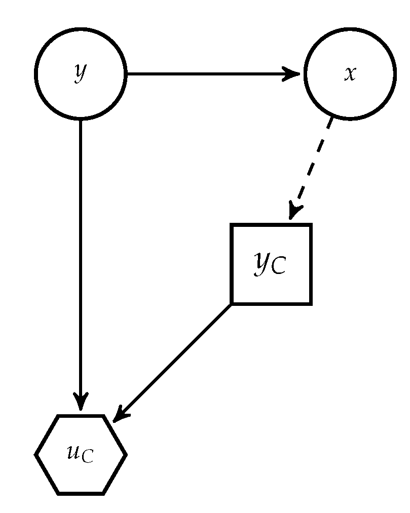
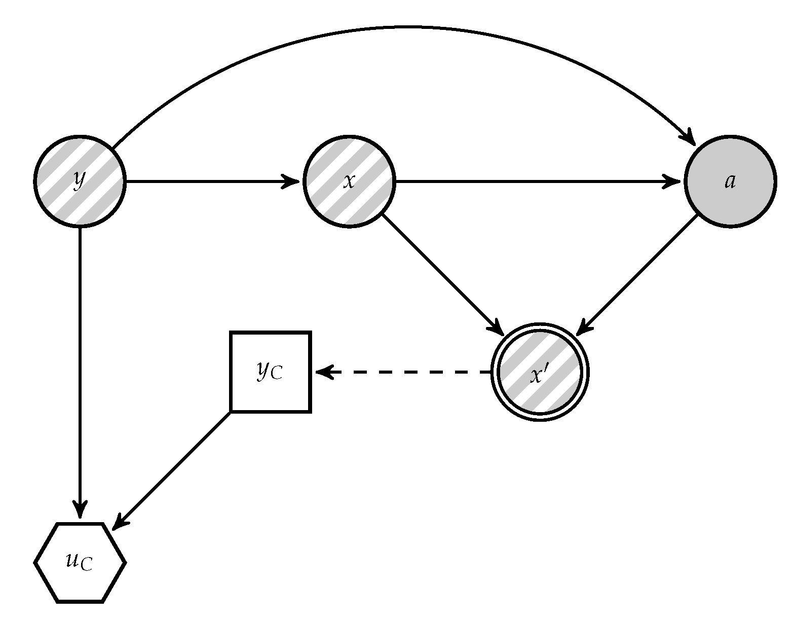
Given the above mentioned issue, we provide ARA solutions to AC. We focus first on modelling the adversary’s problem in the operation phase. We present the classification problem faced by C as a Bayesian decision analysis problem in Figure 3, derived from Figure 2. In it, A’s decision appears as random to the classifier, since she does not know how the adversary will attack the data. For notational convenience, when necessary we distinguish between random variables and realisations using upper and lower case letters, respectively; in particular, we denote by X the random variable referring to the original instance (before the attack) and $X^{\prime }$ that referring to the possibly attacked instance. $\widehat{z}$ will indicate an estimate of z.

An adversary unaware classifier would classify the observed instance $x^{\prime }$ based on

$$arg\underset{y_c}{max}\sum _{i=1}^2{u}_C(y_c,y_i)p_C\left(y_i\right|X=x^{\prime }).$$

(6)

This leads to performance degradation as reflected in Section 2.2. In contrast, an adversary aware classifier would use

$$arg\underset{y_c}{max}\sum _{i=1}^2{u}_C(y_c,y_i)p_C\left(y_i\right|X^{\prime }=x^{\prime }).$$

(7)

In the adversary unaware case, $p_C\left(y_i\right|X=x^{\prime })$ is easily estimated using the training data. However, estimating the probabilities $p_C\left(y_i\right|X^{\prime }=x^{\prime })$ is harder, as it entails modelling how the adversary will modify the original instance x, which is unobserved. Moreover, recall that common knowledge is not available, so we actually lack A’s beliefs and preferences. ARA helps us in modelling our uncertainty about them. In doing so, robustness is typically enhanced. We discuss two strategies depending on whether we use generative or discriminative classifiers as base models.

4.1. The Case of Generative Classifiers

Suppose first that a generative classifier is required. As training data is clean by assumption, we can estimate $p_C\left(y\right)$ (modelling the classifier’s beliefs about the class distribution) and $p_C(X=x|y)$ (modelling her beliefs about the feature distribution given the class when A is not present). In addition, assume that when C observes $X^{\prime }=x^{\prime }$, she can estimate the set ${\mathcal{X}}^{\prime }$ of original instances x potentially leading to the observed $x^{\prime }$. As later discussed, in most applications this will typically be a very large set. When the feature space is endowed with a metric d, an approach to approximate ${\mathcal{X}}^{\prime }$ would be to consider ${\mathcal{X}}^{\prime }=\{x:d(x,x^{\prime })<\rho \}$ for a certain threshold $\rho$.

Given the above, when observing $x^{\prime }$ the classifier should choose the class with maximum posterior expected utility (7). Applying Bayes formula, and ignoring the denominator, which is irrelevant for optimisation purposes, she must find the class

$$\begin{array}{ccc}\hfill y_c^{*}\left(x^{\prime }\right)& =& \underset{y_c}{\arg \max }\sum _{i=1}^2{u}_C(y_c,y)p_C\left(y_i\right)p_C(X^{\prime }=x^{\prime }|y_i)\hfill \\ & =& \underset{y_c}{\arg \max }\sum _{i=1}^2{u}_C(y_c,y_i)p_C\left(y_i\right)\left[\sum _{x\in {\mathcal{X}}^{\prime }}{p}_C(X^{\prime }=x^{\prime }|X=x,y_i)p_C(X=x|y_i)\right].\hfill \end{array}$$

(8)

In such a way, A’s modifications are taken into account through the probabilities $p_C(X^{\prime }=x^{\prime }|X=x,y)$. At this point, recall that the focus is restricted to integrity violation attacks. Then, $p_C(X^{\prime }=x^{\prime }|X=x,y_2)=\delta (x^{\prime }-x)$ and problem (8) becomes

$$\begin{array}{cc}\hfill & \arg {\max }_{y_c}[u_C(y_c,y_1)p_C\left(y_1\right){\sum }_{x\in {\mathcal{X}}^{\prime }}{p}_C(X^{\prime }=x^{\prime }|X=x,y_1)p_C(X=x|y_1)\\ & +u_C(y_c,y_2)p_C\left(y_2\right)p_C(X=x^{\prime }|y_2)].\end{array}$$

(9)

Note that should we assume full common knowledge, we would know A’s beliefs and preferences and, therefore, we would be able to solve his problem exactly: when A receives an instance x from class $y_1$, we could compute the transformed instance. In this case, $p_C\left(X^{\prime }\right|X=x,y_1)$ would be 1 just for the x whose transformed instance coincides with that observed by the classifier and 0, otherwise. Inserting this in (9), we would recover Dalvi’s formulation (5). However, common knowledge about beliefs and preferences does not hold. Thus, when solving A’s problem we have to take into account our uncertainty about his elements and, given that he receives an instance x with label $y_1$, we will not be certain about the attacked output $x^{\prime }$. This will be reflected in our estimate $p_C\left(x^{\prime }\right|x,y_1)$ which will not be 0 or 1 as in Dalvi’s approach (stage 3). With this estimate, we would solve problem (9), summing $p_C\left(x\right|y_1)$ over all possible originating instances, with each element weighted by $p_C\left(x^{\prime }\right|x,y_1)$.

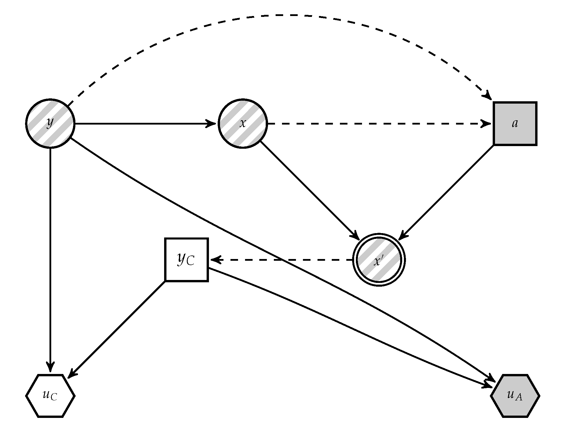
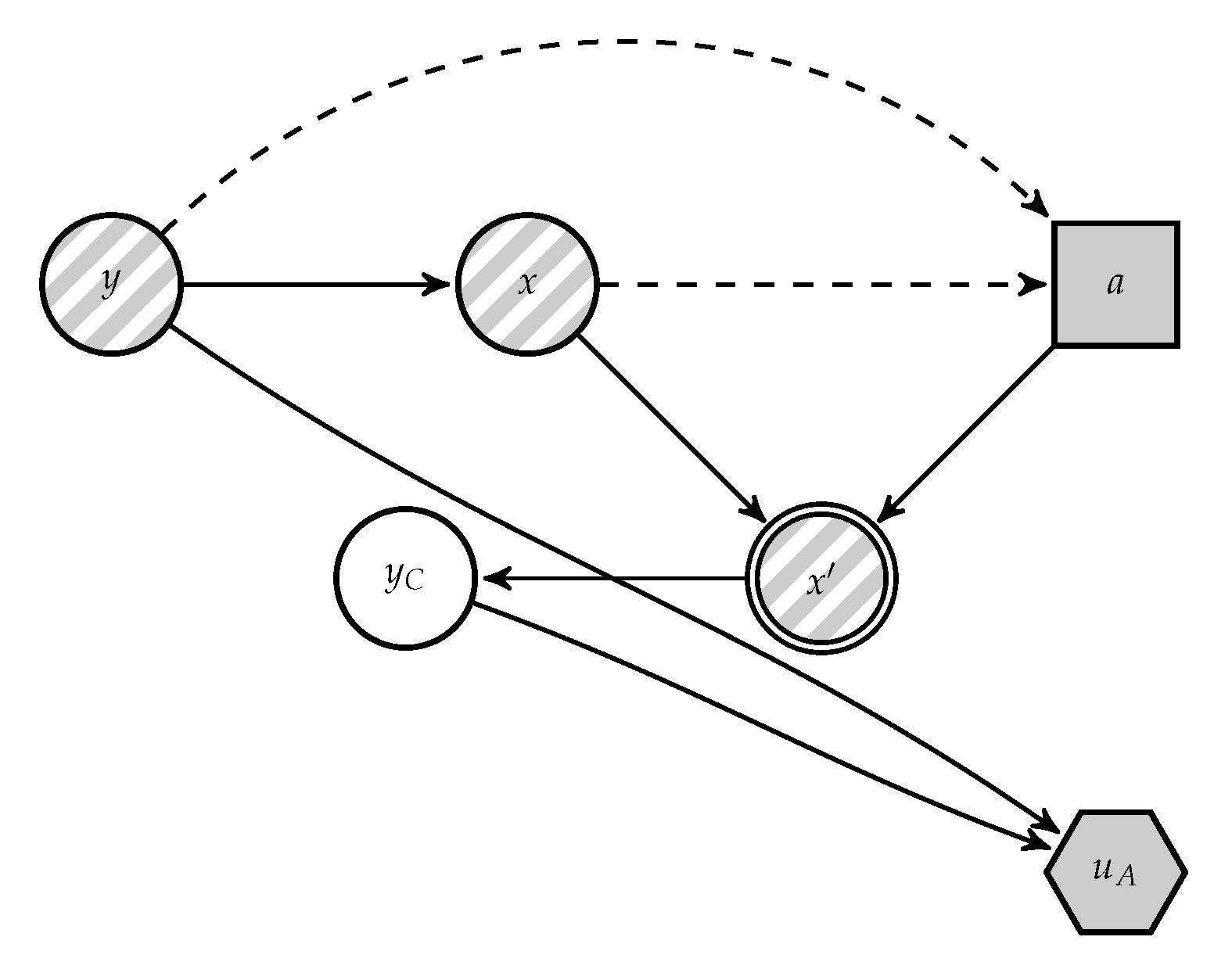
To estimate these last distributions, we resort to A’s problem, assuming that this agent aims at modifying x to maximise his expected utility by making C classify malicious instances as innocent. The decision problem faced by A is presented in Figure 4, derived from Figure 2. In it, C’s decision appears as an uncertainty to A.

To solve the problem, we need $p_A\left(y_c^{*}\left(x^{\prime }\right)\right|x^{\prime })$, which models A’s beliefs about C’s decision when she observes $x^{\prime }$. Let p be the probability $p_A(y_c^{*}\left(a\left(x\right)\right)=y_1|a\left(x\right))$ that A concedes to C saying that the instance is malicious when she observes $x^{\prime }=a\left(x\right)$. Since A will have uncertainty about it, let us model its density using $f_A\left(p\right|x^{\prime }=a\left(x\right))$ with expectation $p_{x^{\prime }=a\left(x\right)}^A$. Then, upon observing an instance x of class $y_1$, A would choose the data transformation maximising his expected utility:

$$\begin{array}{ccc}\hfill x^{\prime }(x,y_1)& \equiv & a^{*}(x,y_1)=\underset{z}{\arg \max }\int [u_A(y_c^{*}\left(z\right)=y_1,y_1)·p\hfill \\ & +& u_A(y_c^{*}\left(z\right)=y_2,y_1)·(1-p)]f_A\left(p\right|z=a\left(x\right))\mathrm{d}p\hfill \\ & =& \underset{z}{\arg \max }\left[u_A(y_1,y_1)-u_A(y_2,y_1)\right]p_{z=a\left(x\right)}^A+u_A(y_2,y_1),\hfill \end{array}$$

(10)

where $u_A(y_i,y_j)$ is the attacker’s utility when the defender classifies an instance of class $y_j$ as one of class $y_i$.

However, the classifier does not know the involved utilities $u_A$ and probabilities $p_{z=a\left(x\right)}^A$ from the adversary. Let us model such uncertainty through a random utility function $U_A$ and a random expectation $P_{z=a\left(x\right)}^A$. Then, we could solve for the random attack, optimising the random expected utility

$$\begin{array}{c}\hfill X^{\prime }(x,y_1)\equiv A^{*}(x,y_1)=\underset{z}{\arg \max }\left(\left[U_A(y_1,y_1)-U_A(y_2,y_1)\right]P_{z=a\left(x\right)}^A+U_A(y_2,y_1)\right).\end{array}$$

We then use such distribution and make (assuming that the set of attacks is discrete, and similarly in the continuous case) $p_C\left(x^{\prime }\right|x,y_1)=Pr(X^{\prime }(x,y_1)=x^{\prime })$ which was the missing ingredient in problem (9). Observe that it could be the case that $Pr(X^{\prime }(x,y_1)=x)>0$, i.e., the attacker does not modify the instance.

Now, without loss of generality, we can associate utility 0 with the worst consequence and 1 with the best one, having the other consequences intermediate utilities. In A’s problem, his best consequence holds when the classifier accepts a malicious instance as innocent (he has opportunities to continue with his operations) while the worst consequence appears when the defender stops an instance (he has wasted effort in a lost opportunity), other consequences being intermediate. Therefore, we adopt $U_A(y_1,y_1)\sim {\delta }_0$ and $U_A(y_2,y_1)\sim {\delta }_1$. Then, the Attacker’s random optimal attack would be

$$X^{\prime }(x,y_1)\equiv A^{*}(x,y_1)=\underset{z}{\arg \max }\left[\left(0-1\right)P_{z=a\left(x\right)}^A+1\right]=\underset{z}{\arg \max }{P}_{z=a\left(x\right)}^A.$$

(11)

Modelling $P_{z=a\left(x\right)}^A$ is more delicate. It entails strategic thinking and could lead to a hierarchy of decision making problems, described in [43] in a simpler context. A heuristic to assess it is based on using the probability $r=P{r}_C(y_c^{*}\left(z\right)=y_1|z)$ that C assigns to the instance received being malicious assuming that she observed z, with some uncertainty around it. As it is a probability, r ranges in $[0,1]$ and we could make $P_{z=a\left(x\right)}^A\sim \beta e({\delta }_1,{\delta }_2)$, with mean ${\delta }_1/({\delta }_1+{\delta }_2)=r$ and variance $\left({\delta }_1{\delta }_2\right)/\left[{({\delta }_1+{\delta }_2)}^2({\delta }_1+{\delta }_2+1)\right]=var$ as perceived. $var$ has to be tuned depending on the amount of knowledge C has about A. Details on how to estimate r are problem dependent.

In general, to approximate $p_C\left(x^{\prime }\right|x,y_1)$ we use Monte Carlo (MC) simulation drawing K samples $\left(P_z^{A,k}\right)$, $k=1,\cdots ,K$ from $P_z^A$, finding $X_k^{\prime }(x,y_1)= \arg {\min }_z{P}_z^{A,k}$ and estimating $p_C\left(x^{\prime }\right|x,y_1)$ using the proportion of times in which the result of the random optimal attack coincides with the instance actually observed by the defender:

$$\begin{array}{c}\hfill {\widehat{p}}_C\left(x^{\prime }\right|x,y_1)=\frac{\#\{X^{\prime }(x,y_1)=x^{\prime }\}}{K}.\end{array}$$

(12)

It is easy to prove, using arguments in [44], that (12) converges almost surely to $p_C\left(x^{\prime }\right|x,y_1)$. In this, and other MC approximations considered, recall that the sample sizes are essentially dictated by the required precision. Based on the Central Limit Theorem [45], MC sums approximate integrals with probabilistic bounds of the order $\sqrt{\frac{var}{N}}$ where N is the MC sum size. To obtain a variance estimate, we run a few iterations and estimate the variance, then choose the required size based on such bounds.

Once we have an approach to estimate the required probabilities, we implement the scheme described through Algorithm 1, which reflects an initial training phase to estimate the classifier and an operational phase which performs the above once a (possibly perturbated) instance $x^{\prime }$ is received by the classifier.

Algorithm 1 General adversarial risk analysis (ARA) procedure for AC. Generative

Input: Training data $D$, test instance $x^{\prime }$. Output: A classification decision $y_c^{*}\left(x^{\prime }\right)$. Training     Train a generative classifier to estimate $p_C\left(y\right)$ and $p_C\left(x\right|y)$ End Training Operation     Read $x^{\prime }$.     Estimate $p_C\left(x^{\prime }\right|x,y_1)$ for all $x\in {\mathcal{X}}^{\prime }$.     Solve $$\begin{array}{ccccc}\hfill y_c^{*}\left(x^{\prime }\right)& =& \underset{y_C}{\arg \max }[u_C(y_C,y_1){\widehat{p}}_C\left(y_1\right)\sum _{x\in {\mathcal{X}}^{\prime }}{\widehat{p}}_C\left(x^{\prime }\right|x,y_1){\widehat{p}}_C\left(x\right|y_1)\hfill & +& u_C(y_C,y_2){\widehat{p}}_C\left(x^{\prime }\right|y_2){\widehat{p}}_C\left(y_2\right)].\end{array}$$     Output $y_c^{*}\left(x^{\prime }\right)$. End Operation

4.2. The Case of Discriminative Classifiers

With discriminative classifiers, we cannot use the previous approach as we lack an estimate of $p_C(X=x|y)$. Alternatively, assume for the moment that the classifier knows the attack that she has suffered and that this is invertible in the sense that she may recover the original instance $x=a^{-1}\left(x^{\prime }\right)$. Then, rather than classifying based on (6), as an adversary unaware classifier would do, she should classify based on

$$\arg \underset{y_c}{\max }\sum _{i=1}^2{u}_C(y_c,y_i)p_C\left(y_i\right|X=a^{-1}\left(x^{\prime }\right)).$$

However, she actually has uncertainty about the attack a, which induces uncertainty about the originating instance x. Suppose we model our uncertainty about the origin x of the attack through a distribution $p_C(X=x|X^{\prime }=x^{\prime })$ with support over the set ${\mathcal{X}}^{\prime }$ of reasonable originating features x. Now, marginalising out over all possible originating instances, the expected utility that the classifier would get for her classification decision $y_c$ would be

$$\begin{array}{ccc}\hfill \psi \left(y_c\right)& =& \sum _{x\in {\mathcal{X}}^{\prime }}\left(\sum _{i=1}^2{u}_C(y_c,y_i)p_C\left(y_i\right|X=x)\right)p_C(X=x|X^{\prime }=x^{\prime })\hfill \\ & =& \sum _{i=1}^2{u}_C(y_c,y_i)\left[\sum _{x\in {\mathcal{X}}^{\prime }}{p}_C\left(y_i\right|X=x)p_C(X=x|X^{\prime }=x^{\prime })\right],\hfill \end{array}$$

(13)

and we would solve for

$$y_c^{*}\left(x^{\prime }\right)=\arg \underset{y_c}{\max }\psi \left(y_c\right).$$

Typically, the expected utilities (13) are approximated by MC using a sample ${\left\{x_n\right\}}_{n=1}^N$ from $p_C\left(x\right|x^{\prime })$. Algorithm 2 summarises a general procedure.

Algorithm 2 General ARA procedure for AC. Discriminative

Input: Monte Carlo size N, training data $D$, test instance $x^{\prime }$. Output: A classification decision $y_c^{*}\left(x^{\prime }\right)$. Training     Based on $D$, train a discriminative classifier to estimate $p_C\left(y\right|x)$. End Training Operation     Read $x^{\prime }$     Estimate ${\mathcal{X}}^{\prime }$ and $p_C\left(x\right|x^{\prime }),x\in {\mathcal{X}}^{\prime }$     Draw sample ${\left\{x_n\right\}}_{n=1}^N$ from $p_C\left(x\right|x^{\prime })$.     Find $y_c^{*}\left(x^{\prime }\right)= \arg {\max }_{y_c}\frac{1}{N}{\sum }_{i=1}^2\left(u_C(y_c,y_i)\left[{\sum }_{n=1}^N{p}_C\left(y_i\right|x_n)\right]\right)$     Output $y_c^{*}\left(x^{\prime }\right)$ End Operation

To implement this approach, we need to be able to estimate ${\mathcal{X}}^{\prime }$ and $p_C\left(x\right|x^{\prime })$ or, at least, sample from such distribution. A powerful approach samples from $p_C\left(X\right|X^{\prime }=x^{\prime })$ by leveraging approximate Bayesian computation (ABC) techniques, [46]. This requires being able to sample from $p_C\left(X\right)$ and $p_C\left(X^{\prime }\right|X=x)$, which we address first.

Estimating $p_C\left(x\right)$ is done using training data, untainted by assumption. For this, we can employ an implicit generative model, such as a generative adversarial network [47] or an energy-based model [48]. In turn, sampling from $p_C\left(x^{\prime }\right|x)$ entails strategic thinking. Notice first that

$$p_C\left(x^{\prime }\right|x)=\sum _{c=1}^2{p}_C\left(x^{\prime }\right|x,y_c)p_C\left(y_c\right|x)=p_C\left(x^{\prime }\right|x,y_1)p_C\left(y_1\right|x)+\delta (x^{\prime }-x)p_C\left(y_2\right|x).$$

We easily generate samples from $p_C\left(y_c\right|x)$, as we can estimate those probabilities based on training data as in Section 2.1. Then, we can obtain samples from $p_C\left(x^{\prime }\right|x)$ sampling $y\sim p_C\left(y\right|x)$ first; next, if $y=y_2$ return x or, otherwise, sample $x^{\prime }\sim p_C\left(x^{\prime }\right|x,y_1)$. To sample from the distribution $p_C\left(x^{\prime }\right|x,y_1)$, we model the problem faced by the attacker when he receives instance x with label $y_1$.The attacker will maximise his expected utility by transforming instance x to $x^{\prime }$ given by (10). Again, associating utility 0 with the attacker’s worst consequence and 1 with the best one; and modelling our uncertainty about the attacker’s estimates of $p_{z=a\left(x\right)}^A$ using random expected probabilities $P_{z=a\left(x\right)}^A$, we would look for random optimal attacks $X^{\prime }(x,y_1)$ as in (11). By construction, if we sample $p_{z=a\left(x\right)}^A\sim P_{z=a\left(x\right)}^A$ and solve

$$x^{\prime } = \underset{z\in {\mathcal{X}}^{\prime }}{\arg \min }{p}_{z=a\left(x\right)}^A,$$

$x^{\prime }$ is distributed according to $p_C\left(x^{\prime }\right|x,y_i)$ which was the last ingredient required.

Once with these two sampling procedures, we generate samples from $p_C\left(X\right|X^{\prime }=x^{\prime })$ with ABC techniques. This entails generating $x\sim p_C\left(X\right)$, ${\tilde{x}}^{\prime }\sim p_C\left(X^{\prime }\right|X=x)$ and accepting x if $\varphi ({\tilde{x}}^{\prime },x^{\prime })<\delta$, where $\varphi$ is a distance function defined in the space of features and $\delta$ is a tolerance parameter. The x generated in this way is distributed approximately according to the desired $p_C\left(x\right|x^{\prime })$. However, the probability of generating samples for which $\varphi ({\tilde{x}}^{\prime },x^{\prime })<\delta$ decreases with the dimension of $x^{\prime }$. One possible solution replaces $x^{\prime }$ by $s\left(x^{\prime }\right)$, a set of summary statistics that capture the relevant information in $x^{\prime }$; then, the acceptance criterion would be replaced by $\varphi (s\left({\tilde{x}}^{\prime }\right),s\left(x^{\prime }\right))<\delta$. The choice of summary statistics is problem specific. We sketch the complete ABC sampling procedure in Algorithm 3, to be integrated within Algorithm 2 in its drawing sample command.

Algorithm 3 ABC scheme to sample from $p_C\left(x\right|x^{\prime })$ within Algorithm 2

Input: Observed instance $x^{\prime }$, data model $p_C\left(x\right)$, $p_C\left(y\right|x)$, $P_z^A$, family of statistics s. Output: A sample approximately distributed according to $p_C\left(x\right|x^{\prime })$. while$\varphi (s\left(x^{\prime }\right),s\left({\tilde{x}}^{\prime }\right))>\delta$do     Sample $x\sim p_C\left(x\right)$     Sample $y\sim p_C\left(y\right|x)$     if $y=y_2$ then         ${\tilde{x}}^{\prime }=x$     else         Sample $p_z^A\sim P_z^A$         Compute ${\tilde{x}}^{\prime }= \arg {\min }_z{p}_z^A$     end if     Compute $\varphi (s\left(x^{\prime }\right),s\left({\tilde{x}}^{\prime }\right))$ end while Output x

5. Scalable Adversarial Classifiers

The approach in Section 4 performs all relevant inference about the adversary during operations. This could be too expensive computationally, especially in applications that require fast predictions based on large scale deep models as motivated by the following image processing problem.

Attacks to neural-based classifiers. Section 3.2 discussed adversarial examples. This kind of attack may harm intensely neural network performance, such as that used in image classification tasks [49]. It has been shown that simple one-pixel attacks can seriously affect performance, [39]. As an example, consider a relatively simple deep neural network (a multilayer perceptron model) [21], trained to predict the handwritten digits in the MNIST dataset [50]. In particular, we used a 2 layer feed-forward neural network with relu activations and a final softmax layer to compute the predictions over the 10 classes. This requires simple extensions from binary to multi-class classification. This network accurately predicts 99% of the digits. Figure 5 provides ten MNIST original samples (top row) and the corresponding images (bottom row) perturbed through FGSM, which are misclassified. For example, the original 0 (first column) is classified as such; however, the perturbed one is not classified as a 0 (more specifically, as an 8) even if it looks as such to the human eye.

Globally, accuracy gets reduced to around 50% (see Figure 6a, curve NONE far right). This suggests a very important performance degradation due to the attack. Section 6.3 continues this example to evaluate the robustification procedure we introduce in Section 5.1

The computational difficulties entailed by the approach in Section 4 stem from two issues:

• Iteration over the set ${\mathcal{X}}^{\prime }$ of potentially originating instances. If no assumptions about attacks are made, this set grows rapidly. For instance, in the spam detection example in Section 2.2, let n be the number of words in the dictionary considered by C to undertake the classification (54 in our spam case). If we assume that the attacker modifies at most one word, the size of ${\mathcal{X}}^{\prime }$ is $\mathcal{O}\left(n\right)$; if he modifies at most two words, it is $\mathcal{O}\left(n^2\right)$, …, and if he modifies at most n words, the number of possible adversarial manipulations (and thus the size of ${\mathcal{X}}^{\prime }$) is $2^n$.
  Even more extremely, in the image processing example we would have to deal with very high-dimensional data (the MNIST images above consist of $28\times 28$ pixels, each taking 256 possible values depending on the gray level). This deems any enumeration over the set ${\mathcal{X}}^{\prime }$ totally unfeasible. In order to tackle this issue, constraints over the attacks could be adopted, for example based on distances.
• Sampling from $p_C\left(x\right|x^{\prime })$. In turn, a huge ${\mathcal{X}}^{\prime }$ renders sampling from this distribution inefficient. As an example, the ABC scheme in Algorithm 3, could converge very slowly requiring careful tuning of the tolerance rate $\delta$. In addition, such algorithm demands the use of an unconditional generative model $p_C\left(x\right)$ to draw realistic samples from the data distribution. This could be computationally demanding, especially when dealing with high-dimensional data.

Therefore, as the key adversary modelling steps are taken during operations, the approach could be inefficient in applications requiring fast predictions.

5.1. Protecting Differentiable Classifiers

Alternatively, learning about the adversary could be undertaken during the training phase as now presented. This provides faster predictions during operations and avoids the expensive step of sampling from $p_C\left(x\right|x^{\prime })$. A relatively weak assumption is made to achieve this: the model can be expressed in parametric probabilistic terms $p_C\left(y\right|x,\beta )$, in a form that is differentiable in the $\beta$ parameters. Mainstream models such as logistic regression or neural networks satisfy such condition, which brings in several benefits. First, we can train the model using SGD or any of its recent variants, such as Adam [51], allowing for scaling to both wide and tall datasets. Then, from SGD we can obtain the posterior distribution of the model by adding a suitable noise term as in SG-MCMC samplers like stochastic gradient Langevin Dynamics (SGLD) [52] or accelerated variants [53].

We require only sampling attacked instances from $p_C\left(x^{\prime }\right|x)$, an attacker model. Depending on the type of data, this model can come through a discrete optimisation problem (as in the attacks of Section 2.2) or a continuous optimisation problem (in which we typically resort to gradient information to obtain the most harmful perturbation as in FGSM). These attacks require white-box access to the defender model, which, as mentioned, is usually unrealistic in security. We mitigate this problem and add realism by incorporating two sources of uncertainties.

1. Defender uncertainty over the attacker model $p_C\left(x^{\prime }\right|x)$. The attacker modifies data in the operation phase. The defender has access only to training data $D$; therefore, she will have to simulate attacker’s actions using such training set. Now, uncertainty can also come from the adversarial perturbation chosen. If the model is also differentiable wrt the input x (as with continuous data such as images or audio), instead of computing a single, optimal and deterministic perturbation, as in AT, we use SGLD to sample adversarial examples from regions of high adversarial loss, adding a noise term to generate uncertainty. Thus, we employ iterates of the form

$$x_{t+1}=x_t-ϵ\mathrm{sign}{\nabla }_{x}log{p}_C\left(y\right|x_t,\beta )+\mathcal{N}(0,2ϵ),$$

(14)

for $t=1,\dots ,T$, where $ϵ$ is a step size. We can also consider uncertainty over the hyperparameters $ϵ$ (say, from a rescaled Beta distribution, since it is unreasonable to consider too high or too low learning rates) and the number T of iterations (say, from a Poisson distribution).

2. Attacker uncertainty over the defender model $p_C\left(y\right|x,\beta )$. It is reasonable to assume that the specific model architecture and parameters are unknown by the attacker. To reflect his uncertainty, he will instead perform attacks over a model $p_C\left(y\right|x,\beta )$ with uncertainty over the values of the model parameters $\beta$, with continuous support. This can be implemented through scalable Bayesian approaches in deep models: the defended model is trained using SGLD, obtaining posterior samples via the iteration

$${\beta }_{t+1}={\beta }_t+\eta {\nabla }_{\beta }log{p}_C\left(y\right|x,{\beta }_t)+\mathcal{N}(0,2\eta ),$$

(15)

with $\eta$ a learning rate, and x sampled either from the set $D$ (untainted) or using an attacker model as in the previous point. We sample maintaining a proportion 1:1 of clean and attacked data.

The previous approaches incorporate some uncertainty about the attacker’s elements to sample from $p_C\left(x^{\prime }\right|x)$. A full ARA sampling from this distribution can be performed as well. Recall that $p_C\left(x^{\prime }\right|x)$ models the classifier’s uncertainty about the attack output when A receives instance x, which stems from the lack of knowledge about A’s utilities and probabilities. Samples from $p_C\left(x^{\prime }\right|x)$ could be obtained as in Section 4.2, enabling explicit modelling of the classifier’s uncertainty about A’s utilities and probabilities.

Algorithm 4 describes how to generate samples incorporating both types of uncertainty previously described. On the whole, it uses the first source to generate perturbations to robustly train the defender’s model based on the second source.

Algorithm 4 Large scale ARA-robust training for AC

Input: Defender model $p_C\left(y\right|x,\beta )$, attacker model $p_C\left(x^{\prime }\right|x)$. Output: A set of k particles ${\left\{{\beta }_i\right\}}_{i=1}^K$ approximating the posterior distribution of the defender model learnt using ARA training. for$t=1$ to T do     Sample $x_1,\dots ,x_K\sim p_C\left(x^{\prime }\right|x)$ with (14) or the approach in Section 4.2 (depending on continuous or discrete data).     ${\beta }_{i,t+1}={\beta }_{i,t}+\eta {\nabla }_{\beta }log{p}_C\left(y\right|x,{\beta }_t)+\mathcal{N}(0,2\eta )$ for each i (SGLD) end for Output $({\beta }_{1,T},\dots ,{\beta }_{K,T}))$

Very importantly, its outcome tends to be more robust than the one we could achieve with just AT protection, since we incorporate some level of adversarial uncertainty. In the end, we collect K posterior samples, ${\left\{{\beta }_k\right\}}_{k=1}^K$, and compute predictive probabilities for a new sample x via marginalisation through $p_C\left(y\right|x)={\displaystyle \frac{1}{K}}{\sum }_{k=1}^K{p}_C\left(y\right|x,{\beta }_k)$, using the previous predictive probability to robustly classify the received instance.

6. Case Study

We use the spam classification dataset from Section 2.2 and the MNIST dataset to illustrate the methods in Section 4 and Section 5. As shown in Section 2.2, simple attacks such as good/bad word insertions are sufficient to critically affect the performance of spam detection algorithms. The small perturbations from Section 5 prove that unprotected image classification systems can easily be fooled by an adversary.

6.1. Ara Defense in Spam Detection Problems

For the first batch of experiments, we use the same classifiers as in Section 5. As a dataset, we use again the UCI Spam Data Set from that section. Once the models to be defended are trained, we perform attacks over the instances in the test set, solving problem (11) for each test spam email, removing the uncertainty that is not present from the adversary’s point of view. He would have uncertainty about $p_{z=a\left(x\right)}^A$, as this quantity depends on the defender’s decision. We test our ARA approach to AC against a worst case attacker who knows the true value of $p_C\left(y\right|x)$ and estimates $p_{z=a\left(x\right)}^A$ through $\frac{1}{M}{\sum }_{n=1}^M{p}_C\left(y_1\right|x_n)$ for a sample ${\left\{x_n\right\}}_{n=1}^M$ from $p^{*}\left(x\right|x^{\prime })$, a uniform distribution over the set of all instances at distance less than or equal to 2 from the observed $x^{\prime }$, using $\varphi (x,x^{\prime })={\sum }_{i=1}^{54}|x_i-x_i^{\prime }|$ as distance function. We employ $M=40$ samples.

To model the uncertainty about $p_z^A$, we use beta distributions centred at the attacker’s probability values with variances chosen to guarantee that the distribution is concave in its support: they must be bounded from above by $min\left\{\left[{\mu }^2(1-\mu )\right]/(1+\mu ),\left[\mu {(1-\mu )}^2\right]/(2-\mu )\right\}$, were $\mu$ is the corresponding mean. We set the variance to be $10\%$ of this upper bound, thus reflecting a moderate lack of knowledge about the attacker’s probability judgements.

Our implementations of Algorithms 2 and 3 use as summary statistics s the 11 most relevant features, with relevance based on permutation importance, [54] (assessing how accuracy decreases when a particular feature is not included). The ABC tolerance $\delta$ is set at 1. Finally, for each instance in the test set we generate 20 samples from $p_C\left(x\right|x^{\prime })$.

Table 2. Accuracy comparison (with precision) of four classifiers on attacked data, with and without ARA-enhanced defence.

Classifier	Acc. Taint.	Acc. ARA Taint.
Naive Bayes	$0.774\pm 0.026$	$0.924\pm 0.004$
Logistic Reg.	$0.681\pm 0.009$	$0.917\pm 0.003$
Neural Net	$0.764\pm 0.007$	$0.811\pm 0.010$
Random Forest	$0.663\pm 0.006$	$0.820\pm 0.005$

compares the ARA performance on tainted data with that of the raw classifiers (from Table 1). As can be seen, our approach allows us to largely heal the performance degradation of the four original classifiers, showcasing the benefits of explicitly modelling the attacker’s behaviour in adversarial environments.

Interestingly, in the case of the naïve Bayes classifier, our ARA approach outperforms the classifier under raw untainted data (Table 1). This effect has been observed also in [12,33] for other algorithms and application areas. This is likely due to the fact that the presence of an adversary has a regularizing effect, being able to improve the original accuracy of the base algorithm and making it more robust.

6.2. Robustified Classifiers in Spam Detection Problems

We next evaluate the scalable approach in Section 5 under the two differentiable models among the previous ones: logistic regression and neural network (with two hidden layers). As required, both models can be trained using SGD plus noise methods to obtain uncertainty estimates from the posterior as in (15). Next, we attack the clean test set using the procedure in Section 2.2 and evaluate the performance of our robustification proposal. Since we are dealing with discrete attacks, we cannot use the uncertainty over attacks as in (14) and just resort to adding the attacker’s uncertainty over the defender model as in (15). To perform classification with this model, we evaluate the Bayesian predictive distribution using 5 posterior samples obtained after SGLD iterations. Results are in

Table 3. Accuracy of two classifiers on clean (untainted), and attacked (tainted) data, with and without robustification.

Classifier	Acc. Unt.	Acc. Tai.	Acc. Rob. Taint.
Logistic Reg.	$0.931\pm 0.007$	$0.705\pm 0.009$	$0.946\pm 0.003$
Neural Net	$0.937\pm 0.005$	$0.636\pm 0.009$	$0.960\pm 0.002$

which include as entries: Acc. Unt. (accuracy over untainted data); Acc. Tai. (it. over tainted data); Acc. Rob. Taint. (it. over tainted data after our robustification adding uncertainties). Note that the first two columns do not coincide with those in Table 1, as we have changed the optimisers to variants of SGD to be amenable to the robustified procedure in Section 5.1.

Observe that the proposed robustification process indeed protects differentiable classifiers, recovering from the degraded performance under attacked data. Moreover, in this example, the robustified classifiers achieve even higher accuracies than those attained by the original classifier over clean data, due to the regularising effect mentioned above.

6.3. Robustified Classifiers in Image Classification Problems

Next, we show the performance of the scalable approach continuing with the digit recognition example from Section 5. This batch of experiments aims to show that the ARA-inspired defence can also scale to high-dimensional feature spaces and multiclass problems. The network architecture is shown in Section 5. It is trained using SGD with momentum ($0.5$) for 5 epochs, with learning rate of $0.01$ and batch size of 32. The training set includes 50,000 digit images, and we report results over a 10,000 digit test set. As for uncertainties from Section 5.1, we use both kinds.

Figure 6 shows the security evaluation curves [7] for three different defences (none, AT and ARA), using two attacks at test time: FGSM and PGD. Such curves depict the accuracy of the defender model at this task (y-axis), under different attack intensities $\alpha$ (x-axis). Note how the uncertainties provided by the ARA training method substantially improve the robustness of the neural network under both attacks. From the graphics, we observe that the ARA approach provides a greater degree of robustness as the attack intensities increase. This suggests that the proposed robustification framework can scale well to both tall and wide datasets and that the introduction of uncertainties by the ARA approach is highly beneficial to increase the robustness of the defended models.

7. Discussion

Adversarial classification aims at enhancing classifiers to achieve robustness in presence of adversarial examples, as usually encountered in many security applications. The pioneering work of [6] framed most later approaches to AC within the standard game theoretic paradigm, in spite of the unrealistic common knowledge assumptions about shared beliefs and preferences required, actually even questioned by those authors. After reviewing them, and analysing their assumptions, we have presented two formal probabilistic approaches for AC based on ARA that mitigate such strong common knowledge assumptions. They are general in the sense that application-specific assumptions are kept to a minimum. We have presented the framework in two different forms: in Section 4, learning about the adversary is performed in the operational phase, with variants for generative and discriminative classifiers. In Section 5, adversarial aspects are incorporated in the training phase. Depending on the particular application, one of the frameworks could be preferred over the other. The first one allows us to make real time inference about the adversary, as it explicitly models his decision making process in operation time; its adaptability is better as it does not need to be retrained every time we need to modify the adversary model. However, this comes at a high computational cost. In applications in which there is a computational bottleneck, the second approach may be preferable, with possible changes in the adversary’s behaviour incorporated via retraining. This tension between the need to robustify algorithms against attacks (training phase, Section 5) and the fast adaptivity of attackers against defences (operational phase, Section 4) is well exemplified in the phishing detection domain as discussed in [2].

Our framework may be extended in several ways. First, we could adapt the proposed approach to situations in which there is repeated play of the AC game, introducing the possibility of learning the adversarial utilities and probabilities in a Bayesian way. Learning over opponent types has been explored with success in reinforcement learning scenarios, [55]. This could be extended to the classification setting. Besides exploratory ones, attacks over the training data [56] may be relevant in certain contexts. In addition, the extension to the case of attacks to innocent instances (not just integrity violation ones) seems feasible using the scalable framework. We have restricted our attention to deterministic attacks, that is, $a^{*}(x,y_1)$ will always lead to $x^{\prime }$; extending our framework to deal with stochastic attacks would entail modelling $p\left(x^{\prime }\right|a^{*},x,y_1)$.

Additional work should be undertaken concerning the algorithmic aspects. In our approach we go through a simulation stage to forecast attacks and an optimisation stage to determine optimal classification. The whole process might be performed through a single stage, possibly based on augmented probability simulation [57].

We have also shown how the robustification procedure from Section 5 can be an efficient way to protect large-scale models, such as those trained using first-order methods. It is well-known that Bayesian marginalisation improves generalisation capabilities of flexible models since the ensemble helps in better exploring the posterior parameter space [58]. Our experiments suggest that this holds also in the domain of adversarial robustness. Thus, bridging the gap between large scale Bayesian methods and Game Theory, as done in the ARA framework, suggests a powerful way to develop principled defences. To this end, strategies to more efficiently explore the highly complex, multimodal posterior distributions of neural models constitute another line of further work.

Lastly, several application areas could benefit highly from protecting their underlying ML models. Spam detectors have been the running example in this article. Malware and phishing detection are two crucial cybersecurity problems in which the data distribution of computer programs is constantly changing, driven by attacker’s interests in evading detectors. Finally, the machine learning algorithms underlying autonomous driving systems need to be robustified from perturbations to their visual processing models and this could be performed through our approaches.

References

1. Bolton, R.J.; Hand, D.J. Statistical fraud detection: A review. Stat. Sci. 2002, 2002, 235–249. [Google Scholar]
2. El Aassal, A.; Bakis, S.; Das, A.; Verma, R. An In-depth benchmarking and evaluation of phishing detection research for security needs. IEEE Access 2020, 8, 22170–22192. [Google Scholar] [CrossRef]
3. Simanjuntak, D.; Ipung, H.; Lim, C.; Nugroho, A. Classification Techniques Used to Faciliate Cyber Terrorism Investigation. In Proceedings of the Second International Conference on Advances in Computing, Control, and Telecommunication Technologies, Washington, DC, USA, 2–4 January 2010; pp. 198–200. [Google Scholar]
4. Merrick, H.; McLay, L. Is Screening Cargo Containers for Smuggled Nuclear Threats Worthwhile? Decis. Anal. 2010, 7, 198–200. [Google Scholar] [CrossRef] [Green Version]
5. Comiter, M. Attacking Artificial Intelligence; Belfer Center Paper: Cambridge, MA, USA, 2019. [Google Scholar]
6. Dalvi, N.; Domingos, P.; Mausam; Sumit, S.; Verma, D. Adversarial classification. In Proceedings of the Tenth ACM SIGKDD International Conference on Knowledge Discovery and Data Mining, KDD ’04, Seattle, WA, USA, 22–25 August 2004; pp. 99–108. [Google Scholar]
7. Biggio, B.; Roli, F. Wild patterns: Ten years after the rise of adversarial machine learning. Pattern Recognit. 2018, 84, 317–331. [Google Scholar] [CrossRef] [Green Version]
8. Zhou, Y.; Kantarcioglu, M.; Xi, B. A survey of game theoretic approach for adversarial machine learning. In Wiley Interdisciplinary Reviews: Data Mining and Knowledge Discovery; Wiley: New York, NY, USA, 2018; p. e1259. [Google Scholar]
9. Antos, D.; Pfeffer, A. Representing Bayesian Games without a Common Prior. In Proceedings AAMAS 2010; van der Hoek, K., Sen, L., Eds.; IFAMAS: Minneapolis, MN, USA, 2010. [Google Scholar]
10. Hargreaves-Heap, S.; Varoufakis, Y. Game Theory: A Critical Introduction; Routledge: London, UK, 2004. [Google Scholar]
11. Rios Insua, D.; Rios, J.; Banks, D. Adversarial risk analysis. J. Am. Stat. Assoc. 2009, 104, 841–854. [Google Scholar] [CrossRef]
12. Naveiro, R.; Redondo, A.; Insua, D.R.; Ruggeri, F. Adversarial classification: An adversarial risk analysis approach. Int. J. Approx. Reason. 2019. [Google Scholar] [CrossRef] [Green Version]
13. Gallego, V.; Naveiro, R.; Redondo, A.; Insua, D.R.; Ruggeri, F. Protecting Classifiers From Attacks. A Bayesian Approach. arXiv 2020, arXiv:2004.08705. [Google Scholar]
14. Huang, L.; Joseph, A.D.; Nelson, B.; Rubinstein, B.I.; Tygar, J.D. Adversarial machine learning. In Proceedings of the 4th ACM Workshop on Security and Artificial Intelligence, AISec ’11, Chicago, IL, USA, 21 October 2011; pp. 43–58. [Google Scholar]
15. Barreno, M.; Nelson, B.; Sears, R.; Joseph, A.D.; Tygar, J.D. Can machine learning be secure? In Proceedings of the 2006 ACM Symposium on Information, Computer and Communications Security, ACM, Singapore, 14–17 April 2006; pp. 16–25. [Google Scholar]
16. Bishop, C.M. Pattern Recognition and Machine Learning; Springer: New York, NY, USA, 2006. [Google Scholar]
17. Rish, I. An empirical study of the naive Bayes classifier. In Proceedings of the IJCAI 2001 Workshop on Empirical Methods in Artificial Intelligence, Seattle, WA, USA, 4–6 August 2001; Volume 3, pp. 41–46. [Google Scholar]
18. Kingma, D.P.; Mohamed, S.; Rezende, D.J.; Welling, M. Semi-supervised learning with deep generative models. In Proceedings of the Advances in Neural Information Processing Systems, Montreal, QC, Canada, 8–13 December 2014; pp. 3581–3589. [Google Scholar]
19. McCullagh, P.; Nelder, J. Generalized Linear Models, 2nd ed.; Chapman and Hall/CRC Monographs on Statistics and Applied Probability Series; Chapman & Hall: London, UK, 1989. [Google Scholar]
20. Bottou, L.; Bousquet, O. The tradeoffs of large scale learning. In Proceedings of the Advances in Neural Information Processing Systems, Vancouver, BC, Canada, 8–11 December 2008; pp. 161–168. [Google Scholar]
21. Goodfellow, I.; Bengio, Y.; Courville, A. Deep Learning; The MIT Press: Wayne, PA, USA, 2016. [Google Scholar]
22. Shachter, R.D. Evaluating Influence Diagrams. Oper. Res. 1986, 34, 871–882. [Google Scholar] [CrossRef]
23. Platt, J. Probabilistic outputs for support vector machines and comparisons to regularized likelihood methods. Adv. Large Margin Classif. 1999, 10, 61–74. [Google Scholar]
24. Hopkins, M.; Reeber, E.; Forman, G.; Suermondt, J. Spambase Data Set. 1999. Available online: https://archive.ics.uci.edu/ml/datasets/Spambase (accessed on 4 November 2020).
25. Park, T.; Casella, G. The Bayesian lasso. J. Am. Stat. Assoc. 2008, 103, 681–686. [Google Scholar] [CrossRef]
26. Kim, J.H. Estimating classification error rate: Repeated cross-validation, repeated hold-out and bootstrap. Comput. Stat. Data Anal. 2009, 53, 3735–3745. [Google Scholar] [CrossRef]
27. Banks, D.; Rios, J.; Rios Insua, D. Adversarial Risk Analysis; Francis Taylor: Orlando, FL, USA, 2015. [Google Scholar]
28. Elkan, C. The Foundations of Cost-Sensitive Learning. In Proceedings of the International Joint Conference on Artificial Intelligence (IJCAI), Seattle, WA, USA, 4–10 August 2001. [Google Scholar]
29. Biggio, B.; Fumera, G.; Roli, F. Security evaluation of pattern classifiers under attack. IEEE Trans. Knowl. Data Eng. 2014, 26, 984–996. [Google Scholar] [CrossRef] [Green Version]
30. Li, B.; Vorobeychik, Y. Feature cross-substitution in adversarial classification. In Proceedings of the Advances in Neural Information Processing Systems, Montreal, QC, Canada, 8–13 December 2014; pp. 2087–2095. [Google Scholar]
31. Lowd, D.; Meek, C. Adversarial learning. In Proceedings of the Eleventh ACM SIGKDD International Conference on Knowledge Discovery in Data Mining, KDD ’05, Chicago, IL, USA, 21–24 August 2005; pp. 641–647. [Google Scholar]
32. Zhou, Y.; Kantarcioglu, M.; Thuraisingham, B.; Xi, B. Adversarial support vector machine learning. In Proceedings of the 18th ACM SIGKDD International Conference on Knowledge Discovery and Data Mining, ACM, Venice, Italy, 24–27 June 2012; pp. 1059–1067. [Google Scholar]
33. Goodfellow, I.J.; Shlens, J.; Szegedy, C. Explaining and harnessing adversarial examples. arXiv 2014, arXiv:1412.6572. [Google Scholar]
34. Vorobeichyk, Y.; Kantarcioglu, M. Adversarial Machine Learning; Morgan Clayton: Los Altos, CA, USA, 2019. [Google Scholar]
35. Kołcz, A.; Teo, C.H. Feature Weighting for Improved Classifier Robustness. In Proceedings of the CEAS’09: Sixth Conference on Email and Anti-Spam, Mountain View, CA, USA, 16–17 July 2009. [Google Scholar]
36. Vorobeychik, Y.; Li, B. Optimal randomized classification in adversarial settings. In Proceedings of the 2014 International Conference on Autonomous Agents and Multi-agent Systems, AAMAS ’14, Paris, France, 5–9 May 2014; pp. 485–492. [Google Scholar]
37. Madry, A.; Makelov, A.; Schmidt, L.; Tsipras, D.; Vladu, A. Towards Deep Learning Models Resistant to Adversarial Attacks. In Proceedings of the International Conference on Learning Representations, Vancouver, BC, Canada, 30 April–3 May 2018. [Google Scholar]
38. Moosavi-Dezfooli, S.M.; Fawzi, A.; Frossard, P. Deepfool: A simple and accurate method to fool deep neural networks. In Proceedings of the IEEE conference on computer vision and pattern recognition, Las Vegas, NV, USA, 27–30 June 2016; pp. 2574–2582. [Google Scholar]
39. Su, J.; Vargas, D.V.; Sakurai, K. One pixel attack for fooling deep neural networks. IEEE Trans. Evol. Comput. 2019, 23, 828–841. [Google Scholar] [CrossRef] [Green Version]
40. Gowal, S.; Dvijotham, K.; Stanforth, R.; Bunel, R.; Qin, C.; Uesato, J.; Arandjelovic, R.; Mann, T.A.; Kohli, P. On the Effectiveness of Interval Bound Propagation for Training Verifiably Robust Models. arXiv 2018, arXiv:1810.12715. [Google Scholar]
41. Kantarcıoğlu, M.; Xi, B.; Clifton, C. Classifier evaluation and attribute selection against active adversaries. Data Min. Knowl. Discov. 2011, 22, 291–335. [Google Scholar] [CrossRef] [Green Version]
42. Großhans, M.; Sawade, C.; Brückner, M.; Scheffer, T. Bayesian games for adversarial regression problems. In Proceedings of the International Conference on Machine Learning, Atlanta, GA, USA, 17–19 June 2013; pp. 55–63. [Google Scholar]
43. Rios, J.; Rios Insua, D. Adversarial Risk Analysis for Counterterrorism Modeling. Risk Anal. 2012, 32, 894–915. [Google Scholar] [CrossRef]
44. Rubinstein, R.Y.; Kroese, D.P. Simulation and the Monte Carlo Method, 3rd ed.; Wiley Publishing: New York, NY, USA, 2016. [Google Scholar]
45. Chung, K. A Course in Probability Theory; Academic Press: New York, NY, USA, 2001. [Google Scholar]
46. Csilléry, K.; Blum, M.G.; Gaggiotti, O.E.; François, O. Approximate Bayesian computation (ABC) in practice. Trends Ecol. Evol. 2010, 25, 410–418. [Google Scholar] [CrossRef]
47. Goodfellow, I.; Pouget-Abadie, J.; Mirza, M.; Xu, B.; Warde-Farley, D.; Ozair, S.; Courville, A.; Bengio, Y. Generative Adversarial Nets. In Advances in Neural Information Processing Systems 27; Ghahramani, Z., Welling, M., Cortes, C., Lawrence, N.D., Weinberger, K.Q., Eds.; Curran Associates, Inc.: Nice, France, 2014; pp. 2672–2680. [Google Scholar]
48. Grathwohl, W.; Wang, K.C.; Jacobsen, J.H.; Duvenaud, D.; Norouzi, M.; Swersky, K. Your classifier is secretly an energy based model and you should treat it like one. In Proceedings of the International Conference on Learning Representations, New Orleans, LA, USA, 6–9 May 2019. [Google Scholar]
49. Szegedy, C.; Zaremba, W.; Sutskever, I.; Bruna, J.; Erhan, D.; Goodfellow, I.; Fergus, R. Intriguing properties of neural networks. arXiv 2013, arXiv:1312.6199. [Google Scholar]
50. Le Cun, Y. The MNIST Database. 1998. Available online: http://yann.lecun.com/exdb/mnist/ (accessed on 4 November 2020).
51. Kingma, D.P.; Ba, J. Adam: A method for stochastic optimization. arXiv 2014, arXiv:1412.6980. [Google Scholar]
52. Welling, M.; Teh, Y.W. Bayesian learning via stochastic gradient Langevin dynamics. In Proceedings of the 28th International Conference on Machine Learning (ICML-11), Bellevue, WA, USA, 28 June–2 July 2011; pp. 681–688. [Google Scholar]
53. Ma, Y.A.; Chen, T.; Fox, E. A complete recipe for stochastic gradient MCMC. In Proceedings of the Advances in Neural Information Processing Systems, Montreal, QC, Canada, 7–12 December 2015; pp. 2917–2925. [Google Scholar]
54. Altmann, A.; Toloşi, L.; Sander, O.; Lengauer, T. Permutation importance: A corrected feature importance measure. Bioinformatics 2010, 26, 1340–1347. [Google Scholar] [CrossRef] [PubMed]
55. Gallego, V.; Naveiro, R.; Insua, D.R.; Oteiza, D.G.U. Opponent Aware Reinforcement Learning. arXiv 2019, arXiv:1908.08773. [Google Scholar]
56. Biggio, B.; Nelson, B.; Laskov, P. Poisoning attacks against support vector machines. arXiv 2012, arXiv:1206.6389. [Google Scholar]
57. Ekin, T.; Naveiro, R.; Torres-Barrán, A.; Ríos-Insua, D. Augmented probability simulation methods for non-cooperative games. arXiv 2019, arXiv:1910.04574. [Google Scholar]
58. Wilson, A.G.; Izmailov, P. Bayesian Deep Learning and a Probabilistic Perspective of Generalization. arXiv 2020, arXiv:2002.08791. [Google Scholar]
Figure 1. Classification as an influence diagram.
Mathematics 08 01957 g001
Figure 2. Adversarial classification as a biagent influence diagram.
Mathematics 08 01957 g002
Figure 3. Classifier problem.
Mathematics 08 01957 g003
Figure 4. Adversary problem.
Mathematics 08 01957 g004
Figure 5. Ten MNIST examples (top) and their perturbations (bottom). Predicted class shown for each example.
Mathematics 08 01957 g005
Figure 6. Robustness of a deep network for MNIST under three defence mechanisms (none, AT, ARA). (a) depicts the security evaluation curves under the FGSM attack. (b) depicts the security evaluation curves under the PGD attack.
Mathematics 08 01957 g006