Some New Facts about the Unit-Rayleigh Distribution with Applications

Abstract

The unit-Rayleigh distribution is a one-parameter distribution with support on the unit interval. It is defined as the so-called unit-Weibull distribution with a shape parameter equal to two. As a particular case among others, it seems that it has not been given special attention. This paper shows that the unit-Rayleigh distribution is much more interesting than it might at first glance, revealing closed-form expressions of important functions, and new desirable properties for application purposes. More precisely, on the theoretical level, we contribute to the following aspects: (i) we bring new characteristics on the form analysis of its main probabilistic and reliability functions, and show that the possible mode has a simple analytical expression, (ii) we prove new stochastic ordering results, (iii) we expose closed-form expressions of the incomplete and probability weighted moments at the basis of various probability functions and measures, (iv) we investigate distributional properties of the order statistics, (v) we show that the reliability coefficient can have a simple ratio expression, (vi) we provide a tractable expansion for the Tsallis entropy and (vii) we propose some bivariate unit-Rayleigh distributions. On a practical level, we show that the maximum likelihood estimate has a quite simple closed-form. Three data sets are analyzed and adjusted, revealing that the unit-Rayleigh distribution can be a better alternative to standard one-parameter unit distributions, such as the one-parameter Kumaraswamy, Topp–Leone, one-parameter beta, power and transmuted distributions.

1. Introduction

In many applied scenarios, we are often confronted with the uncertainty of a phenomenon that can be quantified in a bounded range of values. For the sake of accuracy, proper modeling should take this information into account. As an immediate example, it is natural to model characteristics of the proportion type as a random variable (rv) with values in the “unit interval $(0,1)$”, thus following a certain unit distribution, i.e., distribution with support $(0,1)$. The unit-distributions are of particular interest because of the following argues: (i) any rv X with bounded support of the form $(0,a)$, with $a>0$, can be rescaled on $(0,1)$ as $Y=X/a$, and thus Y follows a certain unit-distribution, (ii) the unit-distributions allow us to define general and simple families of continuous distributions through the composition techniques; if $F\left(x\right)$ denotes a cumulative distribution function (cdf) of a rv following a unit-distribution and $G\left(x\right)$ denotes the cdf of any continuous distribution with support denoted by A, then a valid cdf is given as $H\left(x\right)=F\left(G\right(x\left)\right)$, $x\in \mathbb{R}$, defining a certain family of distributions with support A (see [1] as pioneer reference, as well as [2] for a complete survey in this regard), and (iii) the unit-distributions play a central role to define regression models having some characteristic with unit-interval values (see [3] for the definitions of such regression models and [4] for a focus on the one of most popular of them: the beta regression model).

Among the most useful unit-distributions with various number of parameters, there are the power distribution, beta distribution, Johnson distribution by [5], Topp–Leone distribution by [6], Kumaraswamy distribution by [7], unit-gamma distribution by [8,9], unit-logistic distribution by [10], simplex distribution by [11], unit-Birnbaum–Saunders distribution by [12], exponentiated Kumaraswamy distribution by [13], exponentiated Topp–Leone distribution by [14], unit-Weibull distribution by [15,16], unit-Gompertz by [17], unit-Lindley distribution by [18], unit-inverse Gaussian distribution by [19], composite quantile distributions by [20], unit-generalized half normal distribution by [21], and unit modified Burr-III distribution by [22].

In this paper, we concentrate on a simple one-parameter unit distribution, called the unit-Rayleigh distribution. Technically, this distribution is not new; it corresponds to a special case of the unit-Weibull distribution introduced in [15], and it is briefly presented as such in this reference. However, new researches on the unit-Rayleigh distribution have yielded interesting and surprising mathematical fruits that we share in this paper. Specifically, we provide: (i) new motivations of considering this special distribution, (ii) new characteristics on the form analysis of the corresponding probability density function (pdf) (with a closed form for the mode) and hazard rate function (hrf), revealing an unexpected fitting capability of the unit-Rayleigh model, (iii) new stochastic ordering results involving the power distribution and some unlisted distributions of potential interest, (iv) new manageable expressions and approximations of the incomplete and probability-weighted moments involving the complementary error function, (v) some basics on the distributional properties of the order statistics including discussions on their moments, (vi) a simple expression for the reliability coefficient which is useful for estimation purposes, (vii) a tractable expression and approximation of the so-called Tsallis entropy and (viii) some bivariate extensions of the unit-Rayleigh distribution for two-dimensional modeling objectives. On the practical side, we analyze three different data sets, showing that the unit-Rayleigh distribution can be a better alternative to standard one-parameter unit distributions, such as the one-parameter Kumaraswamy, Topp–Leone, one-parameter beta, power and transmuted distributions.

The paper organization is as follows. Section 2 recalls the unit-Rayleigh distribution, with some new facts related to its main functions. The main technical mathematical results are developed in Section 3. Applications are given in Section 4. Final notes are formulated in Section 5.

2. The Unit-Rayleigh Distribution

This section discusses some new facts regarding the primary essence of the unit-Rayleigh distribution.

2.1. Main Lines of the Study

The block diagram in Figure 1 resumes the main lines of the study.

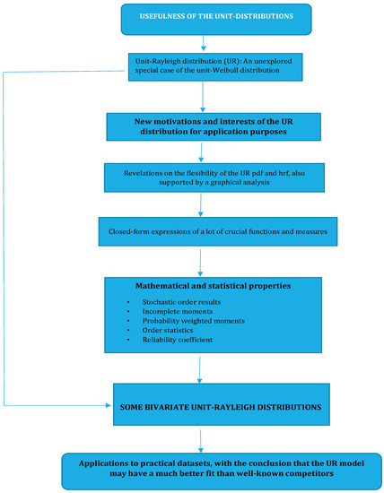
Figure 1. Block diagram on the main lines of this study.

2.2. Corresponding Functions

As the basis, the unit-Rayleigh distribution is associated with the cdf given as

$$\begin{array}{c}\hfill F\left(x\right)=exp\left\{-\beta {\left[log\left(x\right)\right]}^2\right\},x\in (0,1),\end{array}$$

(1)

where $\beta >0$, and $F\left(x\right)=0$ for $x\le 0$ and $F\left(x\right)=1$ for $x>1$. Thus defined, it is a special case of the unit-Weibull distribution introduced by [15] with shape parameter equal to 2. By construction, the unit-Rayleigh distribution is the distribution of the rv $exp(-Y)$, where Y denotes an rv following the Rayleigh distribution with scale parameter $\beta$, i.e., with cdf $F_Y\left(x\right)=1-exp(-\beta x^2)$, with $x>0$, and $F_Y\left(x\right)=0$ otherwise. The Rayleigh distribution also corresponds to the chi-squared distribution with two degrees of freedom. The basics and properties of this distribution can be found in [23].

As a new fact, the unit-Rayleigh distribution is also the distribution of the rv $1/Z$, where Z denotes a rv following the Benini distribution with truncated parameter equal to 1, i.e., with cdf $F_Z\left(x\right)=1-exp\left\{-\beta {\left[log\left(x\right)\right]}^2\right\}$, with $x>1$, and $F_Z\left(x\right)=0$ otherwise. The Benini distribution is a long tail distribution that can be viewed as a generalization of the Pareto distribution. We may refer to the former work of [24].

Based on $F\left(x\right)$, the pdf of the unit-Rayleigh distribution is given as

$$\begin{array}{c}\hfill f\left(x\right)=\frac{d}{dx}F\left(x\right)=-\frac{2\beta }{x}log\left(x\right)exp\left\{-\beta {\left[log\left(x\right)\right]}^2\right\},x\in (0,1),\end{array}$$

(2)

and $f\left(x\right)=0$ for $x\notin (0,1)$. The shape properties of this function are fundamental to evaluate the capability of the unit-Rayleigh model to fit data. This aspect will be discussed later.

The survival function is obtained by

$$\begin{array}{c}\hfill \overline{F}\left(x\right)=1-F\left(x\right)=1-exp\left\{-\beta {\left[log\left(x\right)\right]}^2\right\},x\in (0,1),\end{array}$$

and $\overline{F}\left(x\right)=1$ for $x\le 0$ and $\overline{F}\left(x\right)=0$ for $x>1$, the cumulative hrf is specified as

$$\begin{array}{c}\hfill H\left(x\right)=-log\left[\overline{F}\left(x\right)\right]=-log\left[1-exp\left\{-\beta {\left[log\left(x\right)\right]}^2\right\}\right],x\in (0,1),\end{array}$$

and $H\left(x\right)=0$ for $x\le 0$ and $H\left(x\right)=+\infty$ for $x>1$, and the hrf is given as

$$\begin{array}{c}\hfill h\left(x\right)=\frac{d}{dx}H\left(x\right)=-\frac{2\beta }{x}log\left(x\right)\frac{exp\left\{-\beta {\left[log\left(x\right)\right]}^2\right\}}{1-exp\left\{-\beta {\left[log\left(x\right)\right]}^2\right\}},x\in (0,1),\end{array}$$

(3)

and $h\left(x\right)=0$ for $x\notin (0,1)$. The shape properties of the hrf are precious indicators on some features of the unit-Rayleigh model. This point will be discussed later.

We end this part by specifying the quantile function of the unit-Rayleigh distribution obtained as

$$\begin{array}{c}\hfill Q\left(x\right)=F^{-1}\left(x\right)=exp\left\{-{\left[-\frac{1}{\beta }log\left(x\right)\right]}^{1/2}\right\},x\in (0,1).\end{array}$$

(4)

2.3. Analysis of the cdf

Basically, $F\left(x\right)$ is an increasing and derivable function with respect to x for $x\in (0,1)$. We can express it as a function of the power distribution cdf as

$$F\left(x\right)=F_{*}{\left(x\right)}^{-log\left(x\right)},$$

where $F_{*}\left(x\right)=x^{\beta }$ for $x\in (0,1)$, $F_{*}\left(x\right)=0$ for $x\le 0$ and $F_{*}\left(x\right)=1$ for $x\ge 1$. The following inequalities can be deduced: For any $x\in (0,exp(-1\left)\right)$, we have $F\left(x\right)\le x^{\beta }$, and for $x\in (exp(-1),1)$, the reverse inequality holds: $F\left(x\right)\ge x^{\beta }$.

In addition, we can remark that $F\left(x\right)$ is a decreasing function with respect to $\beta$; by setting $F(x;\beta )=F\left(x\right)$, for any ${\beta }_2\ge {\beta }_1$, we have

$$F(x;{\beta }_2)\le F(x;{\beta }_1).$$

This inequality reveals a basic first-order stochastic dominance of the unit-Rayleigh distribution.

Moreover, one can note that, for any $x\in (0,1)$,

$$\frac{{\partial }^{2}F(x;\beta )}{\partial {\beta }^2}={\left[log\left(x\right)\right]}^{4}exp\left\{-\beta {\left[log\left(x\right)\right]}^2\right\}>0,$$

implying that $F(x;\beta )$ is a convex function with respect to $\beta$.

2.4. Analysis of the pdf

In this section, we analyze $f\left(x\right)$ as described in (2), also performing a mode(s) analysis. Such a global analysis has been performed in [16] for the unit-Weibull distribution, in full generality. Here, we provide more specific details on this aspect for the unit-Rayleigh distribution, including the expression of the mode and its comportment when $\beta$ varied.

As an alpha remark, let us note that, for any $\beta >0$,

$$\underset{x\to 0}{lim}f\left(x\right)=\underset{x\to 1}{lim}f\left(x\right)=0,$$

with the equivalence $f\left(x\right)\sim 2\beta (1-x)$ when $x\to 1$. Since it is positive, the function $f\left(x\right)$ is not monotonic; the points 0 and 1 are not modes of $f\left(x\right)$. Now, for $x\in (0,1)$, we have

$$\begin{array}{c}\hfill \frac{d}{dx}f\left(x\right)=\frac{2\beta }{x^2}exp\left\{-\beta {\left[log\left(x\right)\right]}^2\right\}\left[2\beta {\left[log\left(x\right)\right]}^2+log\left(x\right)-1\right].\end{array}$$

Therefore, a critical point for $f\left(x\right)$, say $x_0$, satisfies $x_0\in (0,1)$ and $2\beta {\left[log\left(x_0\right)\right]}^2+log\left(x_0\right)-1=0$. After developments, we get

$$\begin{array}{c}\hfill x_0=exp\left\{-\frac{1}{4\beta }\left[\sqrt{8\beta +1}+1\right]\right\}.\end{array}$$

(5)

Let us now study the nature of this critical point. For any $x\in (0,1)$, we have

$$\begin{array}{c}\hfill \frac{d^2}{d{x}^2}f\left(x\right)=-\frac{2\beta }{x^3}exp\left\{-\beta {\left[log\left(x\right)\right]}^2\right\}(2\beta log\left(x\right)+1)\left[2\beta {\left[log\left(x\right)\right]}^2+2log\left(x\right)-3)\right].\end{array}$$

Since $(2\beta /x^3)exp\left\{-\beta {\left[log\left(x\right)\right]}^2\right\}>0$, the sign of ${\left.d^{2}f\left(x\right)/d{x}^2\right|}_{x=x_0}$ is the one of

$$\eta =-(2\beta log\left(x_0\right)+1)\left[2\beta {\left[log\left(x_0\right)\right]}^2+2log\left(x_0\right)-3)\right].$$

After developments, we obtain $\eta =-\sqrt{8\beta +1}<0$. We conclude that the point $x_0$ as defined by (5) is a maximum for the function $f\left(x\right)$; it is the (unique) mode of the unit-Rayleigh distribution. Therefore, the pdf of the unit-Rayleigh distribution is “more or less bell shape”.

Let us now discuss the behavior of this mode. By setting $x_0\left(\beta \right)=x_0$, we have

$$\frac{\partial }{\partial \beta }{x}_0\left(\beta \right)=exp\left\{-\frac{1}{4\beta }\left[\sqrt{8\beta +1}+1\right]\right\}\frac{4\beta +\sqrt{8\beta +1}+1}{4{\beta }^2\sqrt{8\beta +1}}>0,$$

implying that $x_0\left(\beta \right)$ is an increasing function with respect to $\beta$. Furthermore, we have

$$\underset{\beta \to 0^{+}}{lim}{x}_0\left(\beta \right)=0,\underset{\beta \to +\infty }{lim}{x}_0\left(\beta \right)=1,$$

meaning that the mode can take all the values of the interval $(0,1)$. This result indicates a certain flexibility of the unit-Rayleigh distribution regarding its mode. A graphical illustration of the possible shapes of $f\left(x\right)$ is provided in Figure 2, considering the following values for $\beta$: $0.1$, $0.5$, $0.8$, $1.5$ and 4.

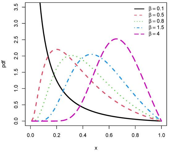
Figure 2. Several curves of the pdf of the unit-Rayleigh distribution.

We see in Figure 2 the “more or less bell shape” of the pdf, with an increasing mode according to $\beta$. Note that the black curve, corresponding to the pdf defined with $\beta =0.1$, is “highly spiked”; the increasing curve does not appear in the figure because it is too sharp. In some senses, this graphical analysis completes the one performed in ([15] Figure 1, last subfigure).

2.5. Analysis of the hrf

In this section, we analyze $h\left(x\right)$ as specified in (3). As far as we know, this aspect has been explored only graphically in ([15] Figure 2, last subfigure). Some new facts are discussed below. Firstly, for any $\beta >0$, we have

$$\underset{x\to 0}{lim}h\left(x\right)=0,\underset{x\to 1}{lim}h\left(x\right)=+\infty ,$$

with the equivalence $h\left(x\right)\sim 2/(1-x)$ when $x\to 1$. Since $h\left(x\right)$ is positive, the point 0 is a minimum for $h\left(x\right)$. Now, for $x\in (0,1)$, we have

$$\begin{array}{c}\hfill \frac{d}{dx}h\left(x\right)=2\beta \frac{w\left(x\right)}{x^2{\left[exp\left\{\beta {\left[log\left(x\right)\right]}^2\right\}-1\right]}^2},\end{array}$$

where

$$w\left(x\right)=2\beta {\left[log\left(x\right)\right]}^{2}exp\left\{\beta {\left[log\left(x\right)\right]}^2\right\}-(1-log\left(x\right))\left[exp\left\{\beta {\left[log\left(x\right)\right]}^2\right\}-1\right],$$

being the difference of two positive functions.

In view of the denominator term, a critical point for $h\left(x\right)$, say $x_1$, satisfies $x_1\in (0,1)$ and $w\left(x_1\right)=0$. The study of this equation is not obvious from the analytical side. As a result, we propose some alternative arguments showing that the hrf can have various forms.

Firstly, due the presence of the $\beta$ in factor of the first term, by dominance, for any $x\in (0,1)$, we have ${lim}_{\beta \to +\infty }w\left(x\right)=+\infty$. This implies the existence of a ${\beta }_{*}$ such that, for $\beta >{\beta }_{*}$, we have $w\left(x\right)>0$ and, a fortiori, $dh\left(x\right)/dx>0$. Hence, for $\beta >{\beta }_{*}$, $h\left(x\right)$ is an increasing function with respect to x. Now, assume that $\beta$ is small, say $\beta \to 0$. Then, standard equivalences gives

$$w\left(x\right)\sim \beta {\left[log\left(x\right)\right]}^2(1+log\left(x\right)),$$

and the equivalence function is equal to 0 if $x=exp(-1)\in (0,1)$. Therefore, in the case where $\beta$ is small enough, at least one critical point exists. This new fact reveals that the hrf is not only an increasing function, as one can think at first sight of ([15] Figure 2, last subfigure); non monotonic shapes are possible for “small or not too small” $\beta$.

We illustrate this new fact by some plots of $h\left(x\right)$ in Figure 2, considering the following values for $\beta$: $0.1$, $0.18$, $0.3$, $0.5$ and $1.5$.

We see in Figure 3 that the hrf can be increasing with convex and concave properties. For the black line corresponding to the hrf defined with $\beta =0.1$, a bathtub shape is observed. These observations confirm the flexible hazard rate of the unit-Rayleigh distribution.

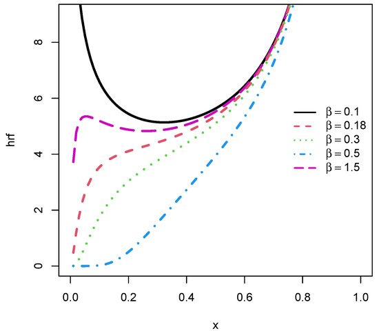
Figure 3. Several curves of the hrf of the unit-Rayleigh distribution.

3. New Results

More mathematical results are developed in this section, all new.

3.1. Stochastic Order Results

We have already presented some stochastic order results involving the cdfs of the unit-Rayleigh and power distributions. More technical ones are described in the result below.

Proposition 1.

The following inequality holds:

$$F_o\left(x\right)\le F\left(x\right)\le F_{oo}\left(x\right),$$

where

• $F_o\left(x\right)=x^{\beta (1/x-1)}$ for $x\in (0,1)$, $F_o\left(x\right)=0$ for $x\le 0$ and $F_o\left(x\right)=1$ for $x\ge 1$,
• $F_{oo}\left(x\right)=x^{\beta (1-x)}$ for $x\in (0,1)$, $F_{oo}\left(x\right)=0$ for $x\le 0$ and $F_{oo}\left(x\right)=1$ for $x\ge 1$,

both being cdfs of unit-distributions.

Proof. 

The inequalities are immediate for $x\le 0$ and $x\ge 1$. For $x\in (0,1)$, we can express $F\left(x\right)$ as $F\left(x\right)=x^{\beta [-log(x\left)\right]}$. The desired result is a consequence of the following well-known inequalities: For $x\in (0,1)$, we have $1-1/x\le log\left(x\right)\le x-1$. The claims that $F_o\left(x\right)$ and $F_{oo}\left(x\right)$ are valid cdfs are proved below. We have ${lim}_{x\to 0}{F}_o\left(x\right)={lim}_{x\to 0}{F}_{oo}\left(x\right)=0$, ${lim}_{x\to 1}{F}_o\left(x\right)={lim}_{x\to 1}{F}_{oo}\left(x\right)=1$, both are derivable for $x\in (0,1)$ with, for $x\in (0,1)$,

$$\begin{array}{c}\hfill \frac{d}{dx}{F}_o\left(x\right)=\beta x^{\beta (1/x-1)-2}[1-x-log\left(x\right)]>0,\frac{d}{dx}{F}_{oo}\left(x\right)=\beta x^{\beta (1-x)-1}[1-x-xlog\left(x\right)]>0.\end{array}$$

This concludes the proof of Proposition 1. ☐

As far as we know, the cdfs $F_o\left(x\right)$ and $F_{oo}\left(x\right)$ described in Proposition 1 are not listed in the literature. They can be of independent interest for purposes out of the scope of this paper (modelling of proportion-type characteristics, constructions of new general families of continuous distributions, etc.).

3.2. Incomplete Moments

The incomplete moments of the unit-Rayleigh remain unexplored. We now fill this gap by providing their analytical expressions via comprehensive functions.

Proposition 2.

Let r be a nonnegative integer and X be a rv following the unit-Rayleigh distribution. Then, the r-th incomplete moment of X at $t\in (0,1)$ is given as

$$\begin{array}{cc}\hfill m_r\left(t\right)& =E\left(X^{r}I\left(\{X\le t\}\right)\right)\hfill \\ \hfill & =t^{r}exp\left\{-\beta {\left[log\left(t\right)\right]}^2\right\}-exp\left(\frac{r^2}{4\beta }\right)\frac{r}{\sqrt{\beta }}\frac{\sqrt{\pi }}{2}\mathrm{erfc}\left(-\sqrt{\beta }log\left(t\right)+\frac{r}{2\sqrt{\beta }}\right),\hfill \end{array}$$

where $I\left(A\right)$ denotes the indicator function over an event A and $\mathrm{erfc}\left(a\right)$ is the complementary error function defined by $\mathrm{erfc}\left(a\right)=(2/\sqrt{\pi }){\int }_a^{+\infty }exp(-y^2)dy$, with $a\in \mathbb{R}$.

Proof. 

We recall that the unit-Rayleigh distribution corresponds to the one of the rv $exp(-Y)$, where Y is a rv following the Rayleigh distribution with scale parameter $\beta$, i.e., with pdf $f_Y\left(x\right)=2\beta xexp(-\beta x^2)$, with $x>0$, and $f_Y\left(x\right)=0$ otherwise. Therefore, we have

$$\begin{array}{cc}\hfill m_r\left(t\right)& =E\left(exp(-rY)I\{exp(-Y)\le t\}\right)=E\left(exp(-rY)I\{Y\ge -log(t\left)\right\}\right)\hfill \\ \hfill & ={\int }_{-log\left(t\right)}^{+\infty }exp(-rx)f_Y\left(x\right)dx=2\beta {\int }_{-log\left(t\right)}^{+\infty }xexp(-rx-\beta x^2)dx\hfill \\ \hfill & =2\beta exp\left(\frac{r^2}{4\beta }\right){\int }_{-log\left(t\right)}^{+\infty }xexp\left\{-{\left(\sqrt{\beta }x+\frac{r}{2\sqrt{\beta }}\right)}^2\right\}dx.\hfill \end{array}$$

By applying the change of variable $y=\sqrt{\beta }x+r/\left(2\sqrt{\beta }\right)$, that is $x=\left[y-r/\left(2\sqrt{\beta }\right)\right]/\sqrt{\beta }$, and performing some calculus, we obtain

$$\begin{array}{cc}\hfill & m_r\left(t\right)=2\beta exp\left(\frac{r^2}{4\beta }\right){\int }_{-\sqrt{\beta }log\left(t\right)+r/\left(2\sqrt{\beta }\right)}^{+\infty }\frac{1}{\sqrt{\beta }}\left(y-\frac{r}{2\sqrt{\beta }}\right)exp(-y^2)\frac{1}{\sqrt{\beta }}dy\hfill \\ \hfill & =2exp\left(\frac{r^2}{4\beta }\right)\left\{{\left[-\frac{1}{2}exp(-y^2)\right]}_{-\sqrt{\beta }log\left(t\right)+r/\left(2\sqrt{\beta }\right)}^{+\infty }-\frac{r}{2\sqrt{\beta }}{\int }_{-\sqrt{\beta }log\left(t\right)+r/\left(2\sqrt{\beta }\right)}^{+\infty }exp(-y^2)dy\right\}\hfill \\ \hfill & =exp\left(\frac{r^2}{4\beta }\right)exp\left\{-{\left(-\sqrt{\beta }log\left(t\right)+\frac{r}{2\sqrt{\beta }}\right)}^2\right\}-exp\left(\frac{r^2}{4\beta }\right)\frac{r}{\sqrt{\beta }}\frac{\sqrt{\pi }}{2}\mathrm{erfc}\left(-\sqrt{\beta }log\left(t\right)+\frac{r}{2\sqrt{\beta }}\right)\hfill \\ \hfill & =t^{r}exp\left\{-\beta {\left[log\left(t\right)\right]}^2\right\}-exp\left(\frac{r^2}{4\beta }\right)\frac{r}{\sqrt{\beta }}\frac{\sqrt{\pi }}{2}\mathrm{erfc}\left(-\sqrt{\beta }log\left(t\right)+\frac{r}{2\sqrt{\beta }}\right).\hfill \end{array}$$

The result of Proposition 2 is obtained. ☐

From Proposition 2, by taking $r=0$, we obtain $m_0\left(t\right)=F\left(t\right)=exp\left\{-\beta {\left[log\left(t\right)\right]}^2\right\}$ with $t\in (0,1)$. The r-th raw moments of X can be derived as

$$\begin{array}{c}\hfill m_r=E\left(X^r\right)=\underset{t\to 1}{lim}{m}_r\left(t\right)=1-exp\left(\frac{r^2}{4\beta }\right)\frac{r}{\sqrt{\beta }}\frac{\sqrt{\pi }}{2}\mathrm{erfc}\left(\frac{r}{2\sqrt{\beta }}\right).\end{array}$$

We thus rediscover the formula in ([15] Subsection 2.2).

In addition, the incomplete moments of X allow us to define an arsenal of interesting measures and functions involving the unit-Rayleigh distribution, such as mean deviations, mean residual life function, variance residual life function, reversed mean residual life function, Zenga curve, and so on. The complete list can be found in the book of [25], among others.

For approximation purposes of the incomplete moments of X, for any $a\in \mathbb{R}$, we can use the well-known expression and approximation of the function erfc(a) given as

$$\mathrm{erfc}\left(a\right)=1-\frac{2}{\sqrt{\pi }}\sum _{j=0}^{+\infty }\frac{{(-1)}^j}{(2j+1)j!}{a}^{2j+1}\approx 1-\frac{2}{\sqrt{\pi }}\sum _{j=0}^J\frac{{(-1)}^j}{(2j+1)j!}{a}^{2j+1},$$

where J denotes a large integer. Let us mention that some more simple approximations of $\mathrm{erfc}\left(a\right)$ exist, with the assumptions that x is “small enough” or “large enough” (see [26]). On the other side, $\mathrm{erfc}\left(a\right)$ is implemented in all the modern mathematical softwares, making the computations of $m_r\left(t\right)$ straightforward.

The following result presents a new and simple series expansion of the incomplete moments, with direct integration; no existing results on $\mathrm{erfc}\left(x\right)$ is used. It thus provides an alternative expression to the one presented in Proposition 2.

Proposition 3.

Under the setting of Proposition 2, for any $t\in (0,1)$, the following series expansion holds:

$$\begin{array}{cc}\hfill & m_r\left(t\right)=\sum _{j=0}^{+\infty }\frac{1}{j!}{(-1)}^j{r}^j{\beta }^{-j/2}\mathrm{\Gamma }\left(\frac{j}{2}+1,\beta {[log\left(t\right)]}^2\right),\hfill \end{array}$$

where $\mathrm{\Gamma }(a,x)$ is the incomplete upper gamma function defined by $\mathrm{\Gamma }(a,x)={\int }_x^{+\infty }{t}^{a-1}exp(-t)dt$, with $a,x>0$.

Proof. 

By making the change of variable $x=Q\left(y\right)$ as defined as (4), we get

$$\begin{array}{cc}\hfill & m_r\left(t\right)={\int }_0^t{x}^{r}f\left(x\right)dx={\int }_0^{F\left(t\right)}{\left[Q\left(y\right)\right]}^{r}dy={\int }_0^{exp\left\{-\beta {\left[log\left(t\right)\right]}^2\right\}}exp\left\{-r{\left[-\frac{1}{\beta }log\left(y\right)\right]}^{1/2}\right\}dy.\hfill \end{array}$$

By applying the Taylor series expansion of the exponential function, we obtain

$$\begin{array}{cc}\hfill & m_r\left(t\right)=\sum _{j=0}^{+\infty }\frac{1}{j!}{(-1)}^j{r}^j{\beta }^{-j/2}{\int }_0^{exp\left\{-\beta {\left[log\left(t\right)\right]}^2\right\}}{\left[-log\left(y\right)\right]}^{j/2}dy.\hfill \end{array}$$

Now, the change of variable $y=exp(-z)$ yields

$$\begin{array}{cc}\hfill & {\int }_0^{exp\left\{-\beta {\left[log\left(t\right)\right]}^2\right\}}{\left[-log\left(y\right)\right]}^{j/2}dy={\int }_{\beta {\left[log\left(t\right)\right]}^2}^{+\infty }{z}^{j/2}exp(-z)dz=\mathrm{\Gamma }\left(\frac{j}{2}+1,\beta {[log\left(t\right)]}^2\right).\hfill \end{array}$$

The proof of Proposition 3 follows from the above equalities. ☐

From Proposition 3, by taking $r=0$ with the convention $0^0=1$ in the sum, we rediscover $m_0\left(t\right)=F\left(t\right)=1\times \mathrm{\Gamma }\left(1,\beta {[log\left(t\right)]}^2\right)=exp\left\{-\beta {\left[log\left(t\right)\right]}^2\right\}$, with $t\in (0,1)$. The r-th raw moments of X can be derived as

$$\begin{array}{c}\hfill m_r=E\left(X^r\right)=\underset{t\to 1}{lim}{m}_r\left(t\right)=\sum _{j=0}^{+\infty }\frac{1}{j!}{(-1)}^j{r}^j{\beta }^{-j/2}\mathrm{\Gamma }\left(\frac{j}{2}+1\right),\end{array}$$

where $\mathrm{\Gamma }\left(a\right)$ is the standard gamma function defined by $\mathrm{\Gamma }\left(a\right)={\int }_0^{+\infty }{t}^{a-1}exp(-t)dt$, with $a>0$.

The following simple finite sum approximation holds:

$$\begin{array}{cc}\hfill & m_r\left(t\right)\approx \sum _{j=0}^J\frac{1}{j!}{(-1)}^j{r}^j{\beta }^{-j/2}\mathrm{\Gamma }\left(\frac{j}{2}+1,\beta {[log\left(t\right)]}^2\right),\hfill \end{array}$$

where J denotes a large integer.

3.3. Probability Weighted Moments

The probability-weighted moments can be viewed as generalizations of raw moments. They appear quite naturally when we deal with the raw moments of order statistics. The closed forms of the probability weighted moments for the unit-Rayleigh distribution are given below.

Proposition 4.

Let r and s be two nonnegative integers and X be a rv following the unit-Rayleigh distribution. Then, the $(r,s)$-th probability weighted moment of X is given as

$$\begin{array}{cc}\hfill m_{r,s}& =E\left[X^{r}F{\left(X\right)}^s\right]=\frac{\beta }{\beta +s}\left[1-exp\left(\frac{r^2}{4(\beta +s)}\right)\frac{r}{\sqrt{\beta +s}}\frac{\sqrt{\pi }}{2}\mathrm{erfc}\left(\frac{r}{2\sqrt{\beta +s}}\right)\right],\hfill \end{array}$$

$\mathrm{erfc}\left(x\right)$ being the complementary error function.

Proof. 

First of all, based on (1) and (2), let us notice that

$$F{\left(x\right)}^{s}f\left(x\right)=-\frac{2\beta }{x}log\left(x\right)exp\left\{-(\beta +s){\left[log\left(x\right)\right]}^2\right\}=\frac{\beta }{\beta +s}{f}_{*}\left(x\right),$$

where $f_{*}\left(s\right)$ denotes the pdf of a rv Z following the unit-Rayleigh distribution with scale parameter $\beta +s$. Therefore

$$\begin{array}{cc}\hfill m_{r,s}& ={\int }_0^1{x}^{r}F{\left(x\right)}^{s}f\left(x\right)dx=\frac{\beta }{\beta +s}{\int }_0^1{x}^r{f}_{*}\left(x\right)dx=\frac{\beta }{\beta +s}E\left(Z^r\right).\hfill \end{array}$$

Owing to Proposition 2 with $\beta +s$ instead of $\beta$ and $t\to 1$, we have

$$\begin{array}{c}\hfill E\left(Z^r\right)=1-exp\left(\frac{r^2}{4(\beta +s)}\right)\frac{r}{\sqrt{\beta +s}}\frac{\sqrt{\pi }}{2}\mathrm{erfc}\left(\frac{r}{2\sqrt{\beta +s}}\right).\end{array}$$

By combining the two equalities above, we conclude the proof of Proposition 4. ☐

Clearly, we have $m_r=m_{r,0}$. The probability-weighted moments will find applications in the next section.

3.4. Order Statistics

The modeling of several physical systems involved the use of order statistics. In this section, the basic properties of the order statistics of the unit-Rayleigh distribution are discussed. The theory and details on order statistics in a general setting can be found in [27].

First, based on a well-known distributional result of order statistics, (1) and (2), the pdf of the u-th order statistic of X in a random sample of size n from the unit-Rayleigh distribution, say $X_{\left(u\right)}$, is

$$\begin{array}{cc}\hfill f_{X_{\left(u\right)}}\left(x\right)& =\frac{n!}{(u-1)!(n-u)!}f\left(x\right)F{\left(x\right)}^{u-1}{[1-F\left(x\right)]}^{n-u}\hfill \\ \hfill & =-\frac{n!}{(u-1)!(n-u)!}\frac{2\beta }{x}log\left(x\right)exp\left\{-\beta u{\left[log\left(x\right)\right]}^2\right\}{\left[1-exp\left\{-\beta {\left[log\left(x\right)\right]}^2\right\}\right]}^{n-u},\hfill \\ \hfill & x\in (0,1).\hfill \end{array}$$

(6)

In particular, for the minimum and maximum order statistics, we get

$$\begin{array}{cc}\hfill f_{X_{\left(1\right)}}\left(x\right)& =-n\frac{2\beta }{x}log\left(x\right)exp\left\{-\beta {\left[log\left(x\right)\right]}^2\right\}{\left[1-exp\left\{-\beta {\left[log\left(x\right)\right]}^2\right\}\right]}^{n-1}\hfill \end{array}$$

and

$$\begin{array}{cc}\hfill f_{X_{\left(n\right)}}\left(x\right)& =-n\frac{2\beta }{x}log\left(x\right)exp\left\{-\beta n{\left[log\left(x\right)\right]}^2\right\},\hfill \end{array}$$

respectively. The raw moments of $X_{\left(u\right)}$ can be simply expressed via the probability weighted moments of the former unit-Rayleigh distribution. Indeed, from the first expression of $f_{X_{\left(u\right)}}\left(x\right)$ in (6) and the binomial formula, we can write

$$\begin{array}{c}\hfill f_{X_{\left(u\right)}}\left(x\right)=\frac{n!}{(u-1)!(n-u)!}\sum _{j=0}^{n-u}\left(\genfrac{}{}{0pt}{}{n-u}{j}\right){(-1)}^{j}f\left(x\right)F{\left(x\right)}^{j+u-1}\end{array}$$

and the r-th raw moment of $X_{\left(u\right)}$ is specified by

$$\begin{array}{cc}\hfill m_{\left(u\right),r}& =E\left(X_{\left(u\right)}^r\right)={\int }_0^1{x}^r{f}_{X_{\left(u\right)}}\left(x\right)dx\hfill \\ \hfill & =\frac{n!}{(u-1)!(n-u)!}\sum _{j=0}^{n-u}\left(\genfrac{}{}{0pt}{}{n-u}{j}\right){(-1)}^j{\int }_0^1{x}^{r}f\left(x\right)F{\left(x\right)}^{j+u-1}dx\hfill \\ \hfill & =\frac{n!}{(u-1)!(n-u)!}\sum _{j=0}^{n-u}\left(\genfrac{}{}{0pt}{}{n-u}{j}\right){(-1)}^j{m}_{r,j+u-1},\hfill \end{array}$$

where, by Proposition 4,

$$\begin{array}{cc}\hfill m_{r,j+u-1}& =\frac{\beta }{\beta +j+u-1}\times \hfill \\ \hfill & \left[1-exp\left(\frac{r^2}{4(\beta +j+u-1)}\right)\frac{r}{\sqrt{\beta +j+u-1}}\frac{\sqrt{\pi }}{2}\mathrm{erfc}\left(\frac{r}{2\sqrt{\beta +j+u-1}}\right)\right].\hfill \end{array}$$

From the raw moments of $X_{\left(u\right)}$, several measures can be derived such as the skewness and kurtosis coefficients, L-moments, allowing to define the L-scale, L-skewness and L-kurtosis, among others.

3.5. Reliability Coefficient

The reliability coefficient allows us to study the behavior of various random systems. It is defined as the probability that a hierarchy exists between two characteristics of the system with unknown values a priori. All the details can be found in [28]. Here, we show that the reliability coefficient can be expressed in a simple manner for the unit-Rayleigh distribution.

Proposition 5.

Let U and V be two independent rvs following the unit-Rayleigh distribution with scale parameters β and ${\beta }_{*}$, respectively. Then, the corresponding reliability coefficient is defined by $R=P(U\le V)$ and

$$\begin{array}{cc}\hfill & R=\frac{{\beta }_{*}}{\beta +{\beta }_{*}}.\hfill \end{array}$$

Proof. 

Let $F(x;\beta )=F\left(x\right)$ be the cdf of U, $f(x;{\beta }_{*})=f\left(x\right)$ be the pdf of V and $f_{*}\left(x\right)$ be the pdf of the unit-Rayleigh distribution with scale parameter $\beta +{\beta }_{*}$. Then, we have

$$\begin{array}{cc}\hfill & R=P(U\le V)={\int }_0^{1}F(x;\beta )f(x;{\beta }_{*})dx={\int }_0^1-\frac{2{\beta }_{*}}{x}log\left(x\right)exp\left\{-(\beta +{\beta }_{*}){\left[log\left(x\right)\right]}^2\right\}dx\hfill \\ \hfill & =\frac{{\beta }_{*}}{\beta +{\beta }_{*}}{\int }_0^1{f}_{*}\left(x\right)dx=\frac{{\beta }_{*}}{\beta +{\beta }_{*}}.\hfill \end{array}$$

This proved Proposition 5. ☐

From Proposition 5, we clearly have $R<1/2$ for ${\beta }_{*}<\beta$, $R=1/2$ for ${\beta }_{*}=\beta$, and $R>1/2$ for ${\beta }_{*}>\beta$. The simple expression of R is useful for statistical aims. In particular, by the invariance property, maximum likelihood estimates of the parameters $\beta$ and ${\beta }_{*}$, say $\widehat{\beta }$ and ${\widehat{\beta }}_{*}$, respectively, provide the maximum likelihood estimate for R given as

$$\widehat{R}=\frac{{\widehat{\beta }}_{*}}{\widehat{\beta }+{\widehat{\beta }}_{*}}.$$

3.6. Tsallis Entropy

Commonly, the Tsallis entropy is a measure of randomness of a random variable. One can refer to the study of [29] for discussions on the roles of various entropy measures in applied sciences, including the Tsallis entropy. The following result concerns a series expansion of this entropy measure in the context of the unit-Rayleigh distribution.

Proposition 6.

Let $\tau \ne 1$ and $\tau >0$. Then, the Tsallis entropy of a random variable X following the unit-Rayleigh distribution can be expressed as

$$\begin{array}{cc}\hfill T_{\tau }& =\frac{1}{\tau -1}\left[1-{\int }_0^{1}f{\left(x\right)}^{\tau }dx\right]\hfill \\ \hfill & =\frac{1}{\tau -1}\left[1-2^{\tau -1}{\beta }^{(\tau -1)/2}{\tau }^{-(\tau +1)/2}\sum _{j=0}^{+\infty }\frac{1}{j!}{(\tau -1)}^j{\beta }^{-j/2}{\tau }^{-j/2}\mathrm{\Gamma }\left(\frac{j+\tau +1}{2}\right)\right].\hfill \end{array}$$

Proof. 

We only need to treat the integral term in the definition of $T_r$. Owing to (2), we have

$$\begin{array}{cc}\hfill {\int }_0^{1}f{\left(x\right)}^{\tau }dx& =2^{\tau }{\beta }^{\tau }{\int }_0^1{x}^{-\tau }{\left[-log\left(x\right)\right]}^{\tau }exp\left\{-\beta \tau {\left[log\left(x\right)\right]}^2\right\}dx.\hfill \end{array}$$

Therefore, by making the change of variable $x=exp(-y)$, i.e., $y=-log\left(x\right)$, and by introducing a rv Y following the Rayleigh distribution with scale parameter $\beta \tau$, we get

$$\begin{array}{cc}\hfill {\int }_0^{1}f{\left(x\right)}^{\tau }dx& =2^{\tau }{\beta }^{\tau }{\int }_0^{+\infty }exp\left[(\tau -1)y\right]y^{\tau }exp(-\beta \tau y^2)dy\hfill \\ \hfill & =2^{\tau -1}{\beta }^{\tau -1}{\tau }^{-1}{\int }_0^{+\infty }exp\left[(\tau -1)y\right]y^{\tau -1}\left[2\beta \tau yexp(-\beta \tau y^2)\right]dy\hfill \\ \hfill & =2^{\tau -1}{\beta }^{\tau -1}{\tau }^{-1}E\left\{exp\left[(\tau -1)Y\right]Y^{\tau -1}\right\}.\hfill \end{array}$$

Now, by using the Taylor series expansion of the exponential function and the following well-known moment properties of the Rayleigh distribution: For any $\upsilon >-2$, $E\left(Y^{\upsilon }\right)={\beta }^{-\upsilon /2}{\tau }^{-\upsilon /2}\mathrm{\Gamma }(\upsilon /2+1)$, we have

$$\begin{array}{cc}\hfill & E\left\{exp\left[(\tau -1)Y\right]Y^{\tau -1}\right\}=\sum _{j=0}^{+\infty }\frac{1}{j!}{(\tau -1)}^{j}E\left(Y^{j+\tau -1}\right)\hfill \\ \hfill & ={\beta }^{-(\tau -1)/2}{\tau }^{-(\tau -1)/2}\sum _{j=0}^{+\infty }\frac{1}{j!}{(\tau -1)}^j{\beta }^{-j/2}{\tau }^{-j/2}\mathrm{\Gamma }\left(\frac{j+\tau +1}{2}\right).\hfill \end{array}$$

By putting the above equalities together, we obtain

$$\begin{array}{cc}\hfill {\int }_0^{1}f{\left(x\right)}^{\tau }dx& =2^{\tau -1}{\beta }^{(\tau -1)/2}{\tau }^{-(\tau +1)/2}\sum _{j=0}^{+\infty }\frac{1}{j!}{(\tau -1)}^j{\beta }^{-j/2}{\tau }^{-j/2}\mathrm{\Gamma }\left(\frac{j+\tau +1}{2}\right).\hfill \end{array}$$

The desired result follows by substituting this series expansion into the former definition of $T_r$. ☐

From Proposition 6, the following approximation holds:

$$\begin{array}{cc}\hfill T_r& \approx \frac{1}{\tau -1}\left[1-2^{\tau -1}{\beta }^{(\tau -1)/2}{\tau }^{-(\tau +1)/2}\sum _{j=0}^J\frac{1}{j!}{(\tau -1)}^j{\beta }^{-j/2}{\tau }^{-j/2}\mathrm{\Gamma }\left(\frac{j+\tau +1}{2}\right)\right],\hfill \end{array}$$

where J is a large enough integer.

3.7. Some Bivariate Unit-Rayleigh Distributions

Now, we present some motivated ideas to construct bivariate unit-Rayleigh distributions, which are of interest for the modelling of conjoint characteristics with values on the unit interval. In order to keep a control on the structure of the marginal rvs, we propose to use the special probabilistic functions called copulas (see [30]).

As a first approach, we can define the Farlie-Gumbel-Morgenstern unit-Rayleigh distribution by the following cdf:

$$\begin{array}{cc}\hfill & F(x,y)=F(x;\beta )F(y;{\beta }_{*})+\lambda F(x;\beta )F(y;{\beta }_{*})\left[1-F(x;\beta )\right]\left[1-F(y;{\beta }_{*})\right],(x,y)\in {\mathbb{R}}^2,\hfill \end{array}$$

where $\lambda \in [-1,1]$, $F(x;\beta )$ and $F(y;{\beta }_{*})$ are defined as (1) with the scale parameters $\beta$ and ${\beta }_{*}$, respectively. Hence, for $(x,y)\in {(0,1)}^2$, we have

$$\begin{array}{cc}\hfill F(x,y)& =exp\left\{-\beta {\left[log\left(x\right)\right]}^2-{\beta }_{*}{\left[log\left(y\right)\right]}^2\right\}+\lambda exp\left\{-\beta {\left[log\left(x\right)\right]}^2-{\beta }_{*}{\left[log\left(y\right)\right]}^2\right\}\times \hfill \\ \hfill & \left[1-exp\left\{-\beta {\left[log\left(x\right)\right]}^2\right\}\right]\left[1-exp\left\{-{\beta }_{*}{\left[log\left(y\right)\right]}^2\right\}\right].\hfill \end{array}$$

By taking $\lambda =0$, the marginal rvs are independent.

Similarly, one can also define a bivariate unit-Rayleigh distribution by using the Clayton copula. Thus, we can define the Clayton unit-Rayleigh distribution by the following cdf:

$$\begin{array}{cc}\hfill & F_{*}(x,y)={\left[max\left(F{(x;\beta )}^{-\lambda }+F{(y;{\beta }_{*})}^{-\lambda }-1,0\right)\right]}^{-1/\lambda },(x,y)\in {\mathbb{R}}^2,\hfill \end{array}$$

where $\lambda \ge -1$ and $\lambda \ne 0$, $F(x;\beta )$ and $F(y;{\beta }_{*})$ are defined as (1) with the scale parameters $\beta$ and ${\beta }_{*}$, respectively. Thus, for $(x,y)\in {(0,1)}^2$, we have

$$\begin{array}{cc}\hfill & F_{*}(x,y)={\left[max\left(exp\left\{\lambda \beta {\left[log\left(x\right)\right]}^2\right\}+exp\left\{\lambda {\beta }_{*}{\left[log\left(y\right)\right]}^2\right\}-1,0\right)\right]}^{-1/\lambda }.\hfill \end{array}$$

As the last example, we can define the Gumbel unit-Rayleigh distribution by the following cdf:

$$\begin{array}{cc}\hfill & F_{**}(x,y)=exp\left\{-{\left[{\left(-log\left[F\right(x;\beta \left)\right]\right)}^{\lambda }+{\left(-log\left[F(y;{\beta }_{*})\right]\right)}^{\lambda }\right]}^{1/\lambda }\right\},(x,y)\in {\mathbb{R}}^2,\hfill \end{array}$$

where $\lambda \ge 1$, $F(x;\beta )$ and $F(y;{\beta }_{*})$ are defined as (1) with the scale parameters $\beta$ and ${\beta }_{*}$, respectively. Hence, for $(x,y)\in {(0,1)}^2$, we have

$$\begin{array}{cc}\hfill & F_{**}(x,y)=exp\left\{-{\left[{\beta }^{\lambda }{\left[log\left(x\right)\right]}^{2\lambda }+{\beta }_{*}^{\lambda }{\left[log\left(y\right)\right]}^{2\lambda }\right]}^{1/\lambda }\right\}.\hfill \end{array}$$

These bivariate extensions generate bivariate models that may be useful in the analysis of compositional data with values over ${(0,1)}^2$, involving proportions and/or percentages. Concrete applications can be found in chemistry, demography, geology, high throughput sequencing and survey. Estimation of the model parameters can be performed via the multivariate likelihood estimation method (see [31]). The detail on the statistical analysis of compositional data can be found in [32,33].

4. Applications

This section shows the applicability behavior of the unit-Rayleigh distribution in a data analysis framework, which has not received a particular attention in [15] or [16]. We estimate the parameter $\beta$ by the maximum likelihood method, as done in [15] but by putting the shape parameter equal to 2; it is not to be estimated. In this case, from n observations of a rv following the unit-Rayleigh distribution, say $x_1,\dots ,x_n$, the maximum likelihood estimate of $\beta$ is defined by

$$\widehat{\beta }={\left\{\frac{1}{n}\sum _{i=1}^n{\left[log\left(x_i\right)\right]}^2\right\}}^{-1}.$$

Based on (1)–(3), the estimated cdf, pdf and hrf are obtained by substituting $\beta$ by $\widehat{\beta }$ in their own expressions.

Thus, with the maximum likelihood method, we aim to compare the fit behavior of the unit-Rayleigh distribution with those of the following well-known one-parameter competitors.

• the one-parameter Kumaraswamy (Ku) distribution (or special Lehmann type II power distribution) defined by the cdf given as

  $$F_{Ku}\left(x\right)=1-{(1-x)}^{\alpha },x\in (0,1),$$
  $F_{Ku}\left(x\right)=0$ for $x\le 0$ and $F_{Ku}\left(x\right)=1$ for $x\ge 1$, with $\alpha >0$. See [7].
• the Topp–Leone (TL) distribution defined by the cdf specified by

  $$F_{TL}\left(x\right)=x^{\theta }{(2-x)}^{\theta },x\in (0,1),$$
  $F_{TL}\left(x\right)=0$ for $x\le 0$ and $F_{TL}\left(x\right)=1$ for $x\ge 1$, where $\theta >0$. See [6].
• the one-parameter beta (B) distribution defined by the cdf given as

  $$F_B\left(x\right)=\frac{1}{B(\mu ,2)}{\int }_0^x{t}^{\mu -1}(1-t)dt,x\in (0,1),$$
  $F_B\left(x\right)=0$ for $x\le 0$ and $F_B\left(x\right)=1$ for $x\ge 1$, where $\mu >0$ and $B(a,b)={\int }_0^1{t}^{a-1}{(1-t)}^{b-1}dt$, $a,b>0$.
• the power (P) distribution defined by the cdf expressed by

  $$F_P\left(x\right)=x^{\eta },x\in (0,1),$$
  $F_P\left(x\right)=0$ for $x\le 0$ and $F_P\left(x\right)=1$ for $x\ge 1$, where $\eta >0$.
• the transmuted (TM) distribution defined by the cdf expressed by

  $$F_{TM}\left(x\right)=(1+\lambda )x-\lambda x^2,x\in (0,1),$$
  $F_{TM}\left(x\right)=0$ for $x\le 0$ and $F_{TM}\left(x\right)=1$ for $x\ge 1$, where $\lambda \in [-1,1]$. We may refer to [34] all the characteristics of the transmuted distribution.

These distributions can be assimilated to semi-parametric statistical models for adjustment purposes. The following classical criteria are used to compare the fits: minus estimated log-likelihood $(-\widehat{\ell })$, consistent Akaike information criterion (CAIC), Hannan–Quinn information criterion (HQIC), Akaike information criterion (AIC), Bayesian information criterion (BIC), Cramer-von Mises criterion (W) and Anderson–Darling criterion (A) are computed. The lower the values of these criteria, the better the fit. The R software developed by [35] is used, with the help of the R function goodness.fit function from the package AdequacyModel (see [36]).

Data with values into $(0,1)$ can be of various natures, including percentages or proportions. Based on positive data $x_1,\dots ,x_n$, one can suppose that a phenomenon can be modeled by a random variable U with estimation of the upper bound of its theoretical support by $m=sup(x_1,\dots ,x_n)$ or any reasonable larger value. Then, we can consider the random variable $X=U/m$ which has support into $(0,1)$. In all the situations, we can recover the distribution of U by multiplication with m a posteriori. In the next, three data sets are considered. The first two data sets used the previous schema, and the third one contains proportions-like data initially communicated with values in $(0,1)$.

First, we consider data of times to infection of kidney dialysis patients in months, as described by [37]. The “times of infection” data set is: {2.5, 2.5, 3.5, 3.5, 3.5, 4.5, 5.5, 6.5, 6.5, 7.5, 7.5, 7.5, 7.5, 8.5, 9.5, 10.5, 11.5, 12.5, 12.5, 13.5, 14.5, 14.5, 21.5, 21.5, 22.5, 22.5, 25.5, 27.5}. Now, we make a normalization operation by divided these data by 30, to get data between 0 and 1. The transformed data set becomes: {0.08333333, 0.08333333, 0.11666667, 0.11666667, 0.11666667, 0.15000000, 0.18333333, 0.21666667, 0.21666667, 0.25000000, 0.25000000, 0.25000000, 0.25000000, 0.28333333, 0.31666667, 0.35000000, 0.38333333, 0.41666667, 0.41666667, 0.45000000, 0.48333333, 0.48333333, 0.71666667, 0.71666667, 0.75000000, 0.75000000, 0.85000000, 0.91666667}.

The second data set concerns the failure times of the air conditioning system of an airplane (in hours), as reported in [38]. These “failure times” data set is: {23, 261, 87, 7, 120, 14, 62, 47, 225, 71, 246, 21, 42, 20, 5, 12, 120, 11, 3, 14, 71, 11, 14, 11, 16, 90, 1, 16, 52, 95}. Again, we make a normalization operation by dividing these data by 265, to get data between 0 and 1. That is, we work with the following data set: {0.086792453, 0.984905660, 0.328301887, 0.026415094, 0.452830189, 0.052830189, 0.233962264, 0.177358491, 0.849056604, 0.267924528, 0.928301887, 0.079245283, 0.158490566, 0.075471698, 0.018867925, 0.045283019, 0.452830189, 0.041509434, 0.011320755, 0.052830189, 0.267924528, 0.041509434, 0.052830189, 0.041509434, 0.060377358, 0.339622642, 0.003773585, 0.060377358, 0.196226415, 0.358490566}.

The third data set is about the maximum flood levels of a particular river in Pennsylvania in millions of cubic feet per second (mlcf/s). It is reported in [39]. With this unity of measure, the data are of proportion type, belonging to $(0,1)$. These “flood levels” data set is: {0.265, 0.269, 0.297, 0.315, 0.3235, 0.338, 0.379, 0.379, 0.392, 0.402, 0.412, 0.416, 0.418, 0.423, 0.449, 0.484, 0.494, 0.613, 0.654, 0.74}

The data sets are basically analyzed in Table 1.

Table 1. Descriptive analysis for the times of infection, failure times and flood levels data sets.

	Units	n	Mean	Median	Variance	Skewness	Kurtosis	Min	Max
Times of infection	months/30	28	0.38	0.3	0.06	0.72	-0.75	0.08	0.92
Failure times	hours/265	30	0.22	0.08	0.07	1.61	1.64	0.003	0.98
Flood levels	mlcf/s	20	0.42	0.41	0.13	0.99	0.25	0.26	0.74

Table 1 indicates that the time of infection data set is right-skewed, with small dispersion and negative kurtosis. This point means that the curve of the unknown pdf behind these data is flatter than a normal pdf. Concerning the failure times data set, we can say that is “significantly” right-skewed, with small dispersion and “significant” kurtosis. For the flood levels data set, we can say that is right-skewed, with small dispersion and slightly positive kurtosis.

So the nature of the three data sets differs in numerous aspects. This is also illustrated through the corresponding boxplots in Figure 4, presenting different quantiles characteristics. Note that some extreme points are present.

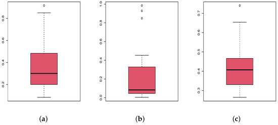
Figure 4. Boxplots of the (a) times of infection data set, (b) failure times data set and (c) flood levels data set.

We complete the first statistical analysis by the total time on test (TTT) plots of the three data sets in Figure 5, Figure 6 and Figure 7, respectively.

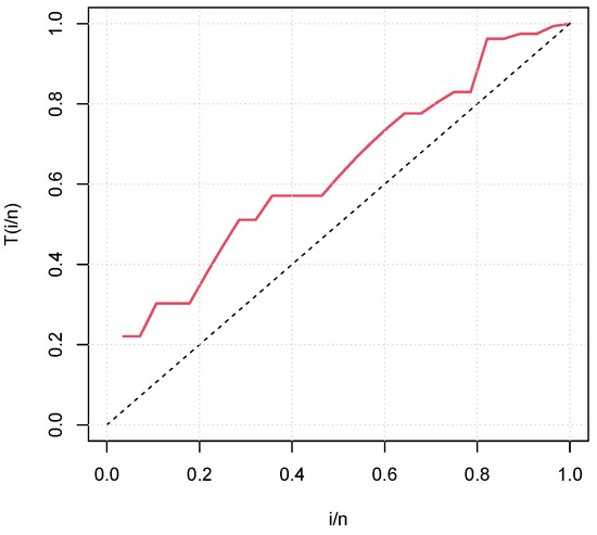
Figure 5. Total time on test (TTT) plot of the times of infection data set.

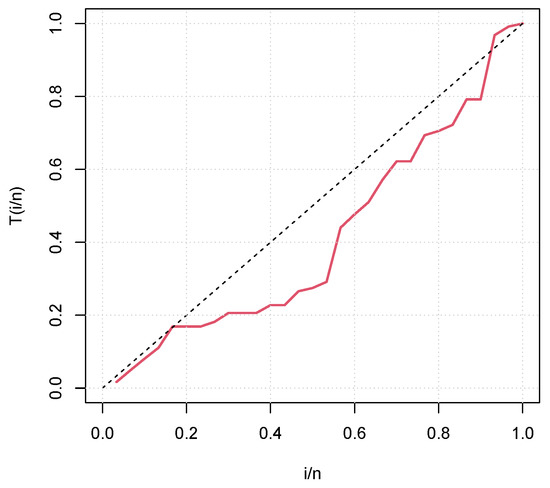
Figure 6. TTT plot of the failure times data set.

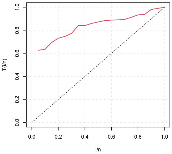
Figure 7. TTT plot of the flood levels data set.

From Figure 5, we see that the TTT curve is concave, which corresponds to an increasing failure intensity for the times of infection data set. Figure 6 shows that the TTT curve is convex, then concave, suggesting a U-shape failure intensity for the failure times data set. In Figure 7, the TTT curve is concave, indicating an increasing failure intensity for the flood levels data set. Thus, these TTT plots highlighted the different nature of the failure intensity of these three data sets. It should also be noted that the increasing and U-shaped failure intensities are covered by the unit-Rayleigh model, which makes it suitable for more suitable analyzes of these data sets.

The quality of fit measurements for the models, as well as the maximum likelihood estimates (MLEs) and standard errors (SEs) of the parameters involved are collected in Table 2, Table 3 and Table 4 for the times of infection, failure times and flood levels data sets, respectively.

Table 2. Criteria and goodness-of-fit measures, maximum likelihood estimates (MLEs) and standard errors (SEs) for the times of infection data set.

Model	$-\widehat{\mathit{\ell }}$	CAIC	HQIC	AIC	BIC	W	A	MLEs (SEs)
UR	−4.4825	−6.8111	−6.557	−6.9650	−5.6328	0.0556	0.3832	0.5221
($\beta$)								(0.0986)
Ku	−3.0686	−3.9834	−3.7300	−4.1373	−2.8051	0.1109	0.6897	1.6615
($\alpha$)								(0.3140)
TL	−3.8524	−5.551	−5.2975	−5.704	−4.3726	0.1066	0.6678	1.3778
($\theta$)								(0.2603)
B	−3.7584	−5.3629	−5.1095	−5.5168	−4.1846	0.1097	0.6839	1.3085
($\mu$)								(0.2151)
TM	−2.9334	−3.7131	−3.4596	−3.8669	−2.5347	0.0963	0.6172	0.7936
($\lambda$)								(0.2721)

CAIC = consistent Akaike information criterion, HQIC = Hannan–Quinn information criterion, AIC = Akaike information criterion, BIC = Bayesian information criterion, W = Cramer-von Mises criterion, A = Anderson–Darling criterion, MLEs = maximum likelihood estimates, SEs = standard errors, UR = unit-Rayleigh, Ku = Kumaraswamy, TL = Topp–Leone, B = beta, P = power, TM = transmuted.

Table 3. Criteria and goodness-of-fit measures, MLEs and SEs for the failure times data set.

Model	$-\widehat{\mathit{\ell }}$	CAIC	HQIC	AIC	BIC	W	A	MLEs (SEs)
UR	−12.7730	−23.4033	−23.0979	−23.5461	−22.1449	0.1253	0.7933	0.1497
($\beta$)								(0.0273)
Ku	−7.5378	−12.9330	−12.627	−13.0759	−11.6747	0.2153	1.3759	2.2333
($\alpha$)								(0.4077)
TL	−11.9801	−21.8175	−21.5121	−21.9603	−20.5591	0.2379	1.5102	0.6017
($\theta$)								(0.1098)
B	−12.0261	−21.9094	−21.6040	−22.0523	−20.6511	0.23084	1.4687	0.6228
($\mu$)								(0.1061)
P	−12.7018	−23.2607	−22.9553	−23.4036	−22.0024	0.2068	1.3212	0.4501
($\eta$)								(0.0821)
TM	−8.4186	−14.6944	−14.3890	−14.8373	−13.4361	0.1764	1.1390	0.8688
($\lambda$)								(0.1318)

Table 4. Criteria and goodness-of-fit measures, MLEs and SEs for the flood level data set.

Model	$-\widehat{\mathit{\ell }}$	CAIC	HQIC	AIC	BIC	W	A	MLEs (SEs)
UR	−11.0858	−19.9494	−19.9773	−20.1716	−19.1759	0.0882	0.5378	1.1383
($\beta$)								(0.2545)
Ku	−2.5115	−2.8009	−2.8287	−3.0231	−2.0273	0.12791	0.7639	1.7276
($\alpha$)								(0.3863)
TL	−7.3674	−12.5126	−12.5404	−12.7348	−11.7390	0.1185	0.7122	2.2446
($\theta$)								(0.5019)
B	−6.4127	−10.6032	−10.63112	−10.8254	−9.8297	0.1238	0.74163	1.8348
($\mu$)								(0.3444)
P	−0.1122	1.9976	2.7711	1.7754	2.7711	0.1220	0.7311	1.1138
($\eta$)								(0.2490)
TW	−2.7473	−3.2724	−3.3003	−3.4946	−2.4989	0.1347	0.8026	1.5451
($\lambda$)								(0.47291)

From Table 2, Table 3 and Table 4, the unit-Rayleigh model can be considered as the best model for the three data sets, because it has the smallest values for the CAIC, HQIC, AIC, BIC, W and A statistics. Figure 8, Figure 9 and Figure 10 confirm this claim through a graphical approach. In them, we plot the estimated pdfs over the adequate histograms for the times of infection, failure times and flood levels data sets, respectively.

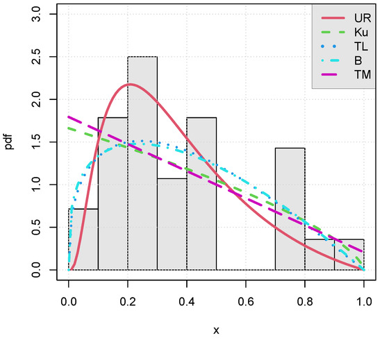
Figure 8. Plots of the estimated pdfs of the considered models for the times of infection data set.

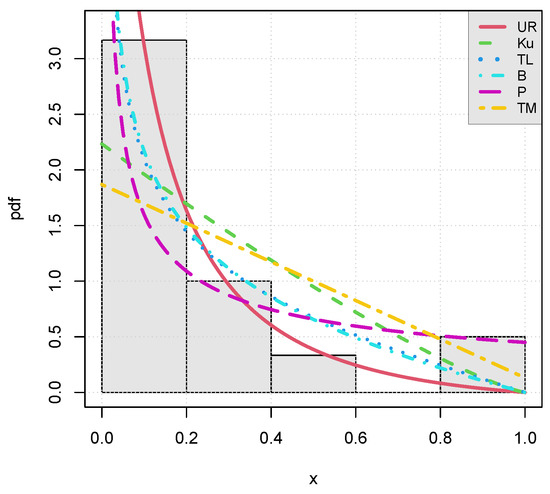
Figure 9. Plots of the estimated pdfs of the considered models for the failure times data set.

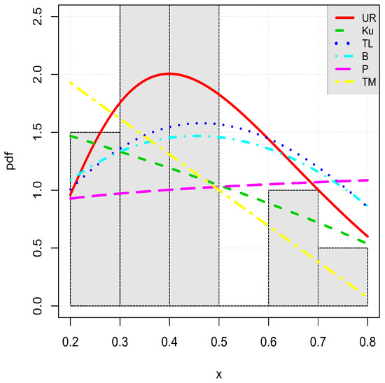
Figure 10. Plots of the estimated pdfs of the considered models for the flood level data set.

As anticipated, Figure 8, Figure 9 and Figure 10 show the nice fits of the unit-Rayleigh model, which has captured the main characteristics of the data contrary to most of the competitors.

We complete this graphical analysis by plotting the estimated hrfs of the unit-Rayleigh model only in Figure 11, Figure 12 and Figure 13.

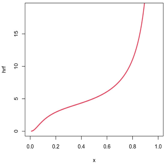
Figure 11. Plots of the estimated hrfs for the times of infection data set.

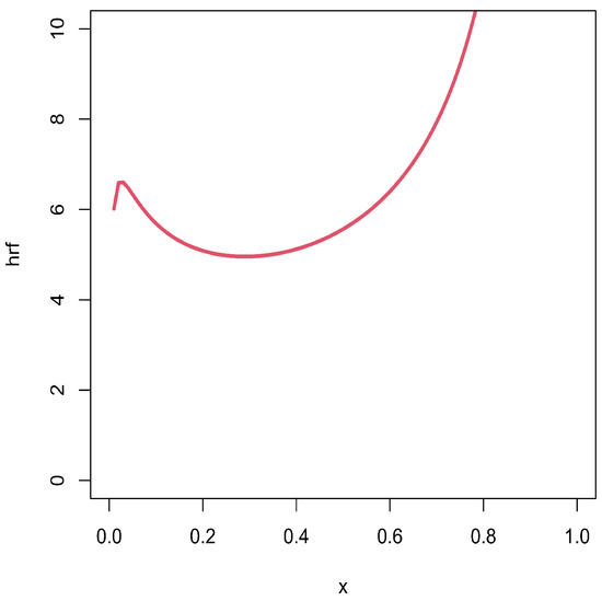
Figure 12. Plots of the estimated hrfs for the failure times data set.

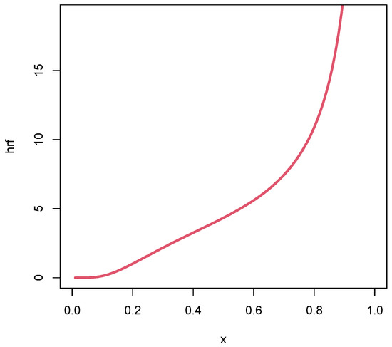
Figure 13. Plots of the estimated hrfs for the flood levels data set.

As expected with the TTT plot in Figure 5, Figure 11 shows an increasing estimated hrf of the unit-Rayleigh model for the times of infection data set. Figure 12 indicates a U-shape estimated hrf for the failure time data set, which is coherent with the observation done in Figure 6. Figure 13 reveals an increasing estimated hrf for the flood levels data set, as anticipated in Figure 7. We thus see the importance of the possible U-shape of the hrf of the unit-Rayleigh distribution as evoked above for such a modelling.

All the preceding points highlight the undeniable capacities of the unit-Rayleigh model in the adjustment of various data. A possible continuation of this work may be the use of the unit-Rayleigh distribution for the construction of general families of distributions, through composition techniques or others, the construction of regression models including characteristics with values on the unit interval through an appropriated link function (see [40]). The presented bivariate versions of the unit-Rayleigh distribution can have applications in the treatment of compositional data with values over ${(0,1)}^2$ (see [32]). All of these research scopes remain to be developed; we leave it for future investigations.

5. Conclusions

In this article, we have shown that the unit-Rayleigh distribution is not only a special case of the unit-Weibull distribution like many others, discussing specific motivations, interests, theoretical results, and practical benefits. In particular, numerous important functions and measures have closed-form expressions that can be useful for various probability and statistical purposes. The most relevant theoretical facts was a detailed analysis of the main functions, results on some stochastic ordering, the expressions of the incomplete and probability weighted moments, as well as those of the Tsallis entropy and reliability coefficient, various properties on the order statistics, and a list of potential bivariate extensions. An applied work has shown how the unit-Rayleigh distribution can be used in practice, with a quite simple estimation of the unique unknown parameter by the maximum likelihood technique. Based on three real data sets, we have proved empirically that it can be superior to other well-reputed one-parameter unit distributions, namely the one-parameter Kumaraswamy, Topp–Leone, one-parameter beta, power and transmuted distributions. We hope that this study will be able to convince applied statisticians, and readers in general, that the unit-Rayleigh distribution can be used effectively in different fields dealing with unit data.

References

- Al-Hussaini, E.K. Composition of cumulative distribution functions. J. Stat. Theory Appl. 2012, 11, 333–336. [Google Scholar]
- Tahir, M.H.; Cordeiro, G.M. Compounding of distributions: A survey and new generalized classes. J. Stat. Distrib. Appl. 2016, 3, 13. [Google Scholar] [CrossRef]
- Kieschnick, R.; McCullough, B.D. Regression analysis of variates observed on (0,1): Percentages, proportions and fractions. Stat. Model. 2003, 3, 193–213. [Google Scholar] [CrossRef]
- Ferrari, S.; Cribari-Neto, F. Beta regression for modelling rates and proportions. J. Appl. Stat. 2004, 31, 799–815. [Google Scholar] [CrossRef]
- Johnson, N.L. Systems of frequency curves generated by methods of translation. Biometrika 1949, 36, 149–176. [Google Scholar] [CrossRef] [PubMed]
- Topp, C.W.; Leone, F.C. A Family of J-shaped frequency functions. J. Am. Stat. Assoc. 1955, 50, 209–219. [Google Scholar] [CrossRef]
- Kumaraswamy, P. A generalized probability density function for double-bounded random processes. J. Hydrol. 1980, 46, 79–88. [Google Scholar] [CrossRef]
- Grassia, A. On a family of distributions with argument between 0 and 1 obtained by transformation of the Gamma distribution and derived compound distributions. Aust. J. Stat. 1977, 19, 108–114. [Google Scholar] [CrossRef]
- Tadikamalla, P.R. On a family of distributions obtained by the transformation of the gamma distribution. J. Stat. Comput. Simul. 1987, 13, 209–214. [Google Scholar] [CrossRef]
- Tadikamalla, P.R.; Johnson, N.L. Systems of frequency curves generated by transfor- mations of logistic variables. Biometrika 1982, 69, 461–465. [Google Scholar] [CrossRef]
- Barndorff-Nielsen, O.; Jorgensen, B. Some parametric models on the Simplex. J. Multivar. Anal. 1991, 39, 106–116. [Google Scholar] [CrossRef]
- Mazucheli, J.; Menezes, A.F.; Dey, S. The unit-Birnbaum-Saunders distribution with applications. Chil. J. Stat. 2018, 9, 47–57. [Google Scholar]
- Lemonte, A.J.; Barreto-Souza, W.; Cordeiro, G.M. The exponentiated Kumaraswamy distribution and its log-transform. Braz. J. Probab. Stat. 2013, 27, 31–53. [Google Scholar] [CrossRef]
- Pourdarvish, A.; Mirmostafaee, S.M.T.K.; Naderi, K. The exponentiated Topp-Leone distribution: Properties and application. J. Appl. Environ. Biol. 2015, 5, 251–256. [Google Scholar]
- Mazucheli, J.; Menezes, A.F.B.; Ghitany, M.E. The unit-Weibull distribution and associated inference. J. Appl. Probab. Stat. 2018, 13, 1–22. [Google Scholar]
- Mazucheli, J.; Menezes, A.F.B.; Fernandes, L.B.; de Oliveira, R.P.; Ghitany, M.E. The unit-Weibull distribution as an alternative to the Kumaraswamy distribution for the modeling of quantiles conditional on covariates. J. Appl. Stat. 2020, 47, 954–974. [Google Scholar] [CrossRef]
- Mazucheli, J.; Menezes, A.F.; Dey, S. Unit-Gompertz distribution with applications. Statistica 2019, 79, 25–43. [Google Scholar]
- Mazucheli, J.; Menezes, A.F.B.; Chakraborty, S. On the one parameter unit-Lindley distribution and its associated regression model for proportion data. J. Appl. Stat. 2019, 46, 700–714. [Google Scholar] [CrossRef]
- Ghitany, M.E.; Mazucheli, J.; Menezes, A.F.B.; Alqallaf, F. The unit-inverse Gaussian distribution: A new alternative to two-parameter distributions on the unit interval. Commun. Stat. Theory Methods 2019, 48, 3423–3438. [Google Scholar] [CrossRef]
- Rodrigues, J.; Bazán, J.L.; Suzuki, A.K. A flexible procedure for formulating probability distributions on the unit interval with applications. Commun. Stat. Theory Methods 2020, 49, 738–754. [Google Scholar] [CrossRef]
- Korkmaz, M.C. The unit generalized half normal distribution: A new bounded distribution with inference and applications. UPB Sci. Bull. Ser. Appl. Math. Phys. 2020, 82, 133–140. [Google Scholar]
- Haq, M.A.; Hashmi, S.; Aidi, K.; Ramos, P.L.; Louzada, F. Unit modified Burr-III distribution: Estimation, characterizations and validation test. Ann. Data Sci. 2020. [Google Scholar] [CrossRef]
- Weisstein, E.W. Rayleigh Distribution, From MathWorld—A Wolfram Web Resource. 2020. Available online: https://mathworld.wolfram.com/RayleighDistribution.html (accessed on 30 October 2020 ).
- Benini, R. I diagrammi a scala logaritmica (a proposito della graduazione per valore delle successioni ereditarie in Italia, Francia e Inghilterra). G. Degli Econ. Serie II 1905, 16, 222–231. [Google Scholar]
- Cordeiro, G.M.; Silva, R.B.; Nascimento, A.D.C. Recent Advances in Lifetime and Reliability Models; Bentham Sciences Publishers: Sharjah, UAE, 2020. [Google Scholar] [CrossRef]
- Decker, D.L. Computer evaluation of the complementary error function. Am. J. Phys. 1975, 43, 833–834. [Google Scholar] [CrossRef]
- David, H.A.; Nagaraja, H. Order Statistics, 3rd ed.; Wiley: New York, NY, USA, 2003. [Google Scholar]
- Surles, J.G.; Padgett, W.J. Inference for reliability and stress-strength for a scaled Burr-type X distribution. Lifetime Data Anal. 2001, 7, 187–200. [Google Scholar] [CrossRef]
- Amigo, J.M.; Balogh, S.G.; Hernandez, S. A brief review of generalized entropies. Entropy 2018, 20, 813. [Google Scholar] [CrossRef]
- Nelsen, R.B. An Introduction to Copulas, 2nd ed.; Springer: Berlin/Heidelberg, Germany, 2006. [Google Scholar]
- Casella, G.; Berger, R.L. Statistical Inference; Brooks/Cole Publishing Company: Bel Air, CA, USA, 1990. [Google Scholar]
- Aitchison, J. The Statistical Analysis of Compositional Data; Chapman and Hall: London, UK, 1986; 416p. [Google Scholar]
- Pawlowsky-Glahn, V.; Egozcue, J.J.; Tolosana-Delgado, R. Modeling and Analysis of Compositional Data; Wiley: New York, NY, USA, 2015. [Google Scholar]
- Shaw, W.T.; Buckley, I.R. The alchemy of probability distributions: beyond Gram-Charlier expansions, and a skew-kurtotic-normal distribution from a rank transmutation Map. arXiv 2009, arXiv:0901.0434. [Google Scholar]
- R Development Core Team. R: A Language and Environment for Statistical Computing; R Foundation for Statistical Computing: Vienna, Austria, 2005; ISBN 3-900051-07-0. Available online: http://www.R-project.org (accessed on 30 October 2020 ).
- Marinho, P.R.D.; Silva, R.B.; Bourguignon, M.; Cordeiro, G.M.; Nadarajah, S. AdequacyModel: An R package for probability distributions and general purpose optimization. PLoS ONE 2019, 14, e0221487. [Google Scholar] [CrossRef]
- Klein, J.P.; Moeschberger, M.L. Survival Analysis: Techniques for Censored and Truncated Data; Springer: Berlin/Heidelberg, Germany, 2006. [Google Scholar]
- Linhart, H.; Zucchini, W. Model Selection; Wiley: New York, NY, USA, 1986. [Google Scholar]
- Dumonceaux, R.; Antle, C.E. Discrimination between the lognormal and Weibull distributions. Technometrics 1973, 15, 923–926. [Google Scholar] [CrossRef]
- Bonat, W.H.; Ribeiro, P.J., Jr.; Zeviani, W.M. Regression models with responses on the unit interval: specification, estimation and comparison. Biom. Braz. J. 2012, 30, 415–431. [Google Scholar]
Publisher’s Note: MDPI stays neutral with regard to jurisdictional claims in published maps and institutional affiliations. |
© 2020 by the authors. Licensee MDPI, Basel, Switzerland. This article is an open access article distributed under the terms and conditions of the Creative Commons Attribution (CC BY) license (http://creativecommons.org/licenses/by/4.0/).