Garch Model Test Using High-Frequency Data


Abstract
1. Introduction
2. The Test of GARCH Model
2.1. The Daily GARCH Model
2.2. The Test of the GARCH Model
2.2.1. The Wald Test
2.2.2. The LR Test
3. The Test of GARCH Model with High-Frequency Data
3.1. A Brief Review of GARCH Model Estimation Using High-Frequency Data
3.2. The Test of GARCH Model Using High-Frequency Data
3.2.1. The Wald Test
3.2.2. The LR Test
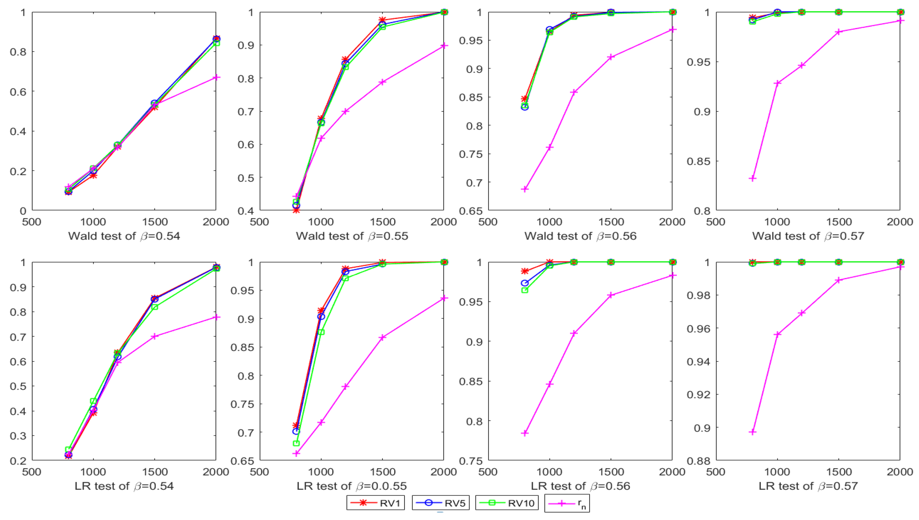
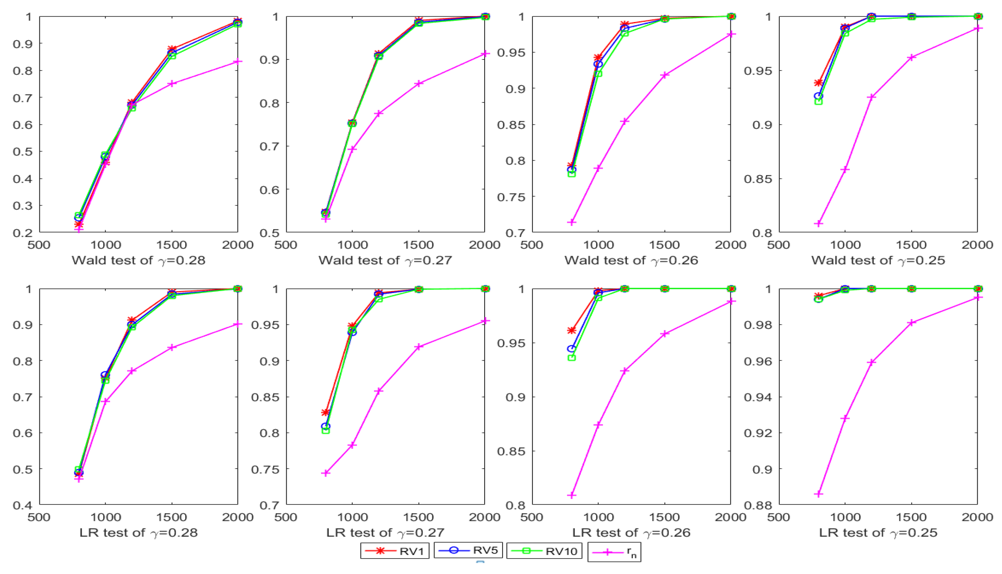
4. Simulation Study
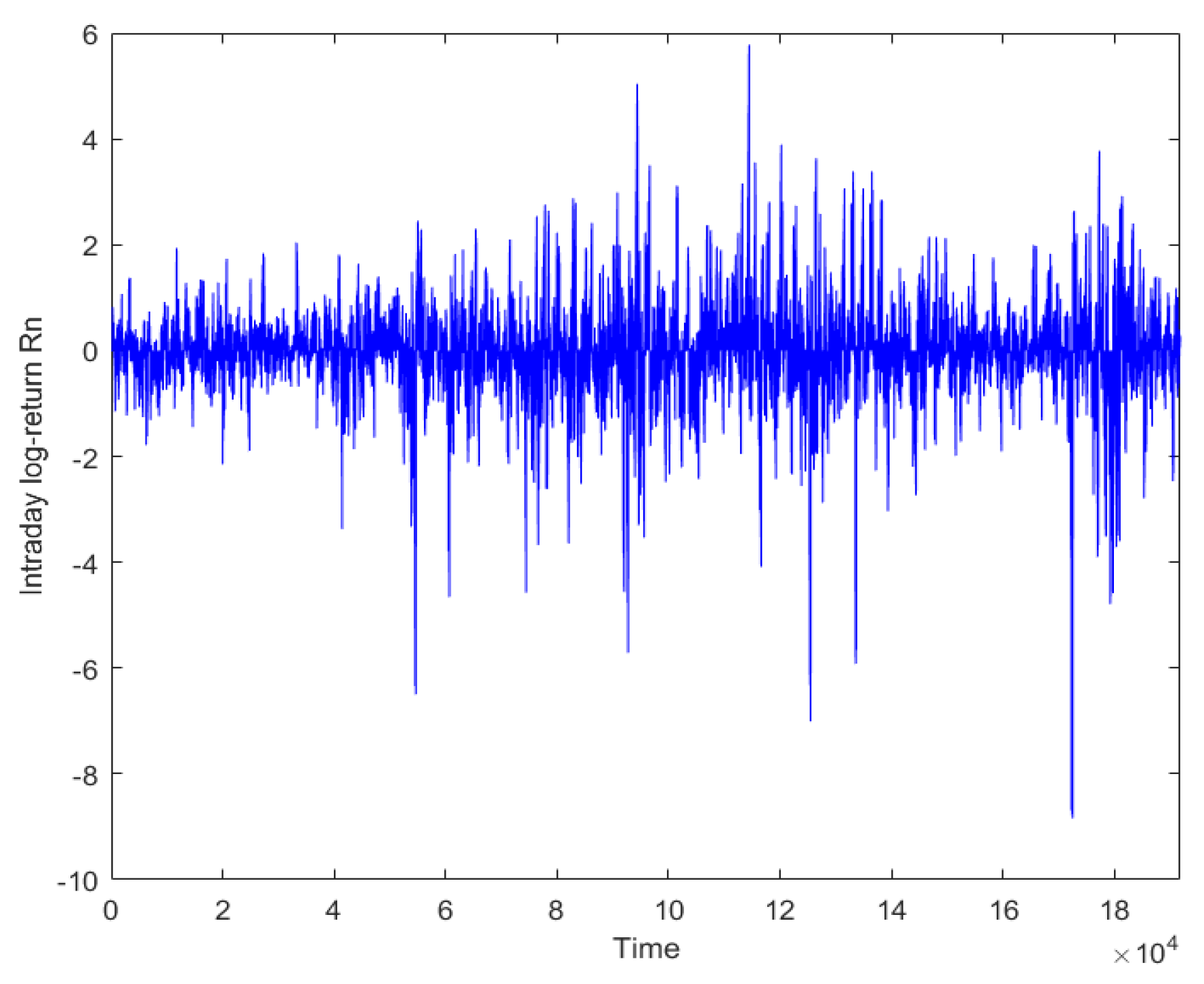
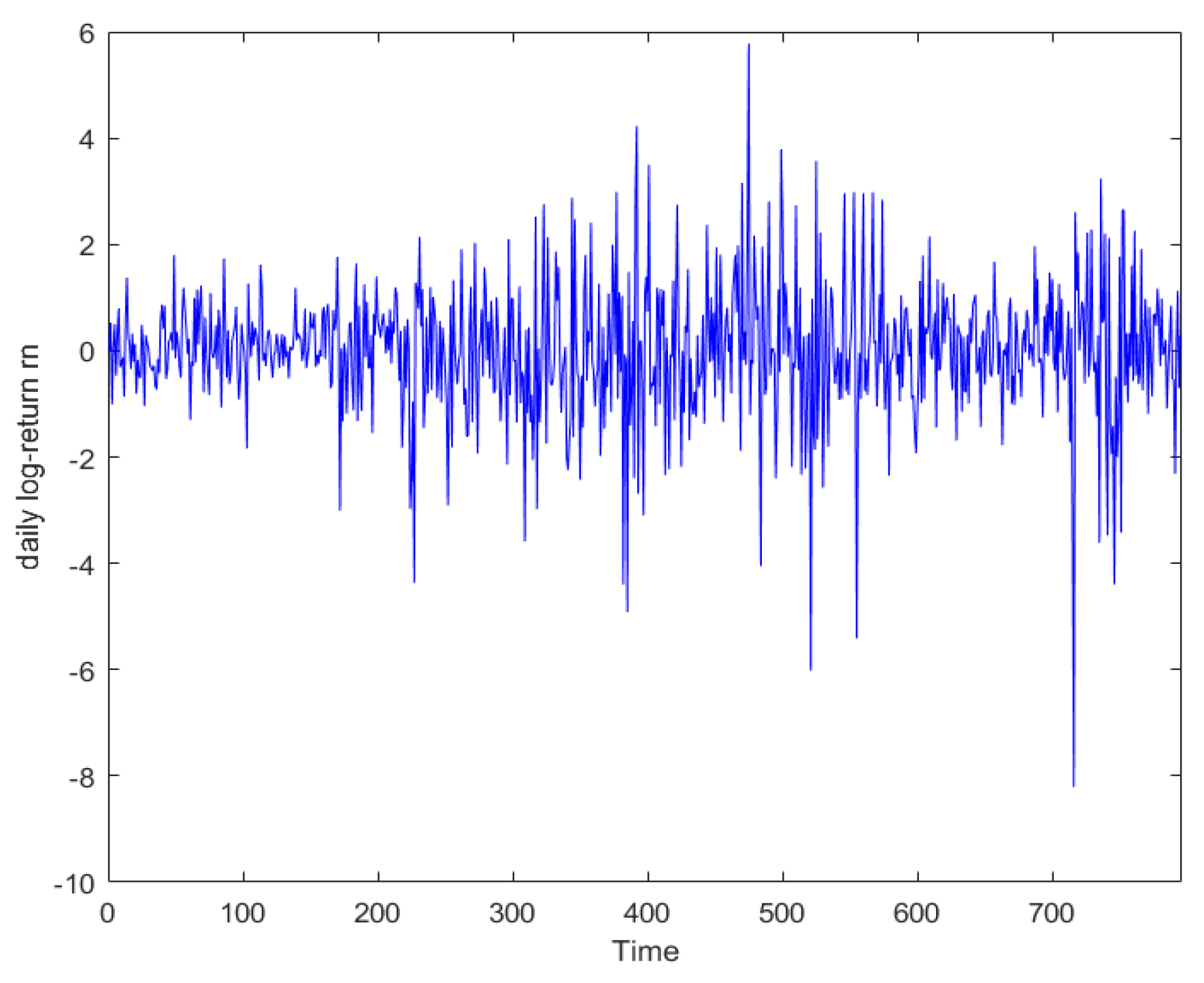
5. Empirical Study
6. Conclusions
Author Contributions
Funding
Acknowledgments
Conflicts of Interest
Appendix A
- (A1)
- is an i.i.d sequence with ;
- (A2)
- is a compact subset of the space given by , , , and int;
- (A3)
- ;
- (A4)
- is a non-degenerate random variable;
- (A5)
- .
- (B1)
- is compact, has nonempty interior and int;
- (B2)
- The variance functions are measurable functions of the data for all and are twice continuously differentiable with respect to on int;
- (B3)
- satisfies the UWLLN and is the identifiably unique maximizer (see [45]) of
- (B4)
- The Hessian satisfies the UWLLN and the expected Hessian is positive definite;
- (B5)
- The outer product of satisfies the UWLLN, and the expected outer product is positive definite.
Appendix B
Appendix B.1. Proof of Theorem 1
Appendix B.2. Proof of Theorem 2
References
- Narsoo, J. High Frequency Exchange Rate Volatility Modelling Using the Multiplicative Component GARCH. Int. J. Stat. Appl. 2016, 6, 8–14. [Google Scholar]
- Engle, R. Autoregressive conditional heteroskedasticity with estimates of the variance of U.K. inflation. Econometrica 1982, 50, 987–1007. [Google Scholar] [CrossRef]
- Bollerslev, T. Generalized autoregressive conditional heteroskedasticity. J. Econ. 1986, 31, 307–327. [Google Scholar] [CrossRef]
- Engle, R.F.; Bollerslev, T. Modelling the persistence of conditional variances. Econ. Rev. 1986, 5, 1–50. [Google Scholar] [CrossRef]
- Nelson, D. Conditional heteroscedasticity in stock returns: A new approach. Econometrica 1991, 59, 703–708. [Google Scholar] [CrossRef]
- Glosten, L.R.; Jagannathan, R.; Runkle, D.E. On the relation between the expected value and the volatility of the nominal excess return on stocks. J. Financ. 1993, 48, 1779–1801. [Google Scholar] [CrossRef]
- Bollerslev, T.; Mikkelsen, H.O. Modeling and pricing long memory in stock market volatility. J. Econ. 1996, 73, 151–184. [Google Scholar] [CrossRef]
- Francq, C.; Zakoïan, J.M. Maximum likelihood estimation of pure GARCH and ARMA-GARCH processes. Bernoulli 2004, 10, 605–637. [Google Scholar] [CrossRef]
- Francq, C.; Zakoïan, J.M. The L2-structures of standard and switching-regime GARCH models. Stoch. Process. Appl. 2005, 115, 1557–1582. [Google Scholar] [CrossRef]
- Huang, J.J.; Lee, K.J.; Liang, H.; Lin, W.F. Estimating value at risk of portfolio by conditional copula-GARCH method. Insur. Math. Econ. 2009, 45, 315–324. [Google Scholar] [CrossRef]
- Chan, F.; Theoharakis, B. Estimating m-regimes STAR-GARCH model using QMLE with parameter transformation. Math. Comput. Simul. 2011, 81, 1385–1396. [Google Scholar] [CrossRef]
- Li, D.; Zhang, X.; Zhu, K.; Ling, S. The ZD-GARCH model: A new way to study heteroscedasticity. J. Econ. 2018, 202, 1–17. [Google Scholar] [CrossRef]
- Takaishi, T. Volatility estimation using a rational GARCH model. Quant. Financ. Econ. 2018, 2, 127–136. [Google Scholar] [CrossRef]
- Francq, C.; Zakoïan, J.M. GARCH Models: Structure, Statistical Inference and Financial Applications; John Wiley & Sons, Ltd.: West Sussex, UK, 2010; pp. 141–201. [Google Scholar]
- Wood, R.A.; Mcinish, T.H.; Ord, J.K. An Investigation of Transactions Data for NYSE Stocks. J. Financ. 1985, 25, 723–739. [Google Scholar] [CrossRef]
- Harris, R. Home ownership and class in modern Canada. Int. J. Urban Reg. Res. 1986, 10, 67–86. [Google Scholar] [CrossRef]
- Baillie, R.T.; Bollerslev, T. IntraDay and InterMarket Volatility in Foreign Exchange Rates. Rev. Econ. Stud. 1991, 58, 565–585. [Google Scholar] [CrossRef]
- Goodhart, C.A.; O’Hara, M. High frequency data in financial markets: Issues and applications. J. Empir. Financ. 1997, 4, 73–114. [Google Scholar] [CrossRef]
- Barndorff-Nielsen, O.E.; Shephard, N. Estimating quadratic variation using realized variance. J. Appl. Econ. 2002, 17, 457–477. [Google Scholar] [CrossRef]
- Andersen, T.G.; Bollerslev, T.; Diebold, F.X.; Labys, P. Modeling and Forecasting Realized Volatility. Econometrica 2003, 71, 579–625. [Google Scholar] [CrossRef]
- Hansen, P.R.; Huang, Z.; Shek, H.H. Realized GARCH: A Joint Model for Returns and Realized Measures of Volatility. J. Appl. Econ. 2012, 27, 877–906. [Google Scholar] [CrossRef]
- Hansen, P.R.; Lunde, A.; Voev, V. Realized beta GARCH: A multivariate GARCH model with realized measures of volatility. J. Appl. Econ. 2014, 29, 774–799. [Google Scholar] [CrossRef]
- Hansen, P.R.; Huang, Z. Exponential GARCH Modeling With Realized Measures of Volatility. J. Bus. Econ. Stat. 2016, 34, 269–287. [Google Scholar] [CrossRef]
- Andersen, T.G.; Bollerslev, T. Intraday periodicity and volatility persistence in financial markets. J. Empir. Financ. 1997, 4, 115–158. [Google Scholar] [CrossRef]
- Andersen, T.G.; Bollerslev, T. Answering the Skeptics: Yes, Standard Volatility Models do Provide Accurate Forecasts. Int. Econ. Rev. 1998, 39, 885–905. [Google Scholar] [CrossRef]
- Visser, M.P. Garch Parameter Estimation Using High-Frequency Data. J. Financ. Econ. 2011, 9, 162–197. [Google Scholar] [CrossRef][Green Version]
- Huang, J.; Wu, W.; Chen, Z.; Zhou, J. Robust M-estimate of GJR Model with High Frequency Data. Acta Math. Appl. Sin. 2015, 31, 591–606. [Google Scholar] [CrossRef]
- Wang, M.; Chen, Z.; Wang, C.D. Composite Quantile Regression For GARCH Models Using High-Frequency Data. Econ. Stat. 2017, 7, 115–133. [Google Scholar] [CrossRef]
- Fan, P.; Lan, Y.; Chen, M. The estimating method of VaR based on PGARCH model with high-frequency data. Syst. Eng. Theory Pract. 2017, 37, 2052–2059. [Google Scholar]
- Mariani, M.; Bhuiyan, M.; Tweneboah, O.; Gonzalez-Huizar, H.; Florescu, I. Volatility models applied to geophysics and high frequency fnancial market data. Physica A 2018, 15, 1–32. [Google Scholar]
- Gyamerah, S.A. Modelling the volatility of Bitcoin returns using GARCH models. Quant. Financ. Econ. 2019, 3, 739–753. [Google Scholar] [CrossRef]
- Bhuiyan, M.A.M. Predicting Stochastic Volatility For Extreme Fluctuations In High Frequency Time Series. Open Access Theses Diss. 2020, 2934, 1–77. [Google Scholar]
- Lee, J.H.H. A Lagrange multiplier test for GARCH models. Econ. Lett. 1991, 37, 265–271. [Google Scholar] [CrossRef]
- Berkes, I.; Horváth, L.; Kokoszka, P. Testing for parameter constancy in GARCH(p,q) models. Stat. Probab. Lett. 2004, 70, 263–273. [Google Scholar] [CrossRef]
- Lee, S.; Song, J. Test for parameter change in ARMA models with GARCH innovations. Stat. Probab. Lett. 2008, 78, 1990–1998. [Google Scholar] [CrossRef]
- Carbon, M.; Francq, C. Portmanteau goodness-of-fit test for asymmetric power GARCH models. Austrian J. Stat. 2010, 40, 55–64. [Google Scholar]
- Gel, Y.R.; Chen, B. Robust Lagrange multiplier test for detecting ARCH/GARCH effect using permutation and bootstrap. Can. J. Stat. 2012, 40, 405–426. [Google Scholar] [CrossRef]
- Leucht, A.; Kreiss, J.P.; Neumann, M.H. A Model Specification Test For GARCH(1,1) Processes. Scand. J. Stats 2016, 42, 1167–1193. [Google Scholar] [CrossRef]
- Xiong, Q.; Hu, Z.; Li, Y. Statistic inference for a single-index ARCH-M model. Commun. Stat. Theory Methods 2018, 47, 102–117. [Google Scholar] [CrossRef]
- Straumann, D.; Mikosch, T. Quasi-Maximum-Likelihood Estimation in Conditionally Heteroscedastic Time Series: A Stochastic Recurrence Equations Approach. Ann. Stat. 2006, 34, 2449–2495. [Google Scholar] [CrossRef]
- Engle, R.F. Chapter 13 Wald, likelihood ratio, and Lagrange multiplier tests in econometrics. Handb. Econ. 1984, 2, 775–826. [Google Scholar]
- Scott, L.O. Option Pricing when the Variance Changes Randomly: Theory, Estimation, and an Application. J. Financ. Quant. Anal. 1987, 22, 419–438. [Google Scholar] [CrossRef]
- Wooldridge, J.M. A Unified Approach to Robust, Regression-Based Specification Tests. Econ. Theory 1990, 6, 17–43. [Google Scholar] [CrossRef]
- Bollerslev, T.; Wooldridge, J. Quasi Maximum Likelihood Estimation and Inference in Dynamic Models with Time Varying Covariances. Econ. Rev. 1992, 11, 143–172. [Google Scholar] [CrossRef]
- Bates, C. A Unified Theory of Consistent Estimation for Parametric Models. Econ. Theory 1985, 1, 151–175. [Google Scholar] [CrossRef]


| N | Test | True Value | |||
|---|---|---|---|---|---|
| 800 | Ward | 0.069 | 0.076 | 0.078 | 0.085 |
| LR | 0.067 | 0.066 | 0.076 | 0.079 | |
| 1000 | Ward | 0.063 | 0.065 | 0.070 | 0.076 |
| LR | 0.052 | 0.053 | 0.056 | 0.066 | |
| 1200 | Ward | 0.039 | 0.045 | 0.051 | 0.064 |
| LR | 0.049 | 0.054 | 0.057 | 0.067 | |
| 1500 | Ward | 0.045 | 0.049 | 0.049 | 0.058 |
| LR | 0.047 | 0.05 | 0.051 | 0.053 | |
| 2000 | Ward | 0.046 | 0.048 | 0.054 | 0.059 |
| LR | 0.052 | 0.055 | 0.056 | 0.062 | |
| N | Test | ||||||||
| 800 | Wald | 0.093 | 0.096 | 0.108 | 0.119 | 0.401 | 0.416 | 0.426 | 0.442 |
| LR | 0.217 | 0.222 | 0.245 | 0.226 | 0.712 | 0.701 | 0.680 | 0.662 | |
| 1000 | Wald | 0.177 | 0.200 | 0.212 | 0.211 | 0.677 | 0.666 | 0.663 | 0.618 |
| LR | 0.392 | 0.407 | 0.439 | 0.402 | 0.914 | 0.904 | 0.876 | 0.717 | |
| 1200 | Wald | 0.320 | 0.330 | 0.329 | 0.317 | 0.857 | 0.844 | 0.832 | 0.700 |
| LR | 0.634 | 0.617 | 0.633 | 0.595 | 0.988 | 0.983 | 0.971 | 0.780 | |
| 1500 | Wald | 0.519 | 0.542 | 0.532 | 0.531 | 0.975 | 0.962 | 0.954 | 0.788 |
| LR | 0.854 | 0.850 | 0.818 | 0.700 | 0.999 | 0.996 | 0.996 | 0.867 | |
| 2000 | Wald | 0.867 | 0.864 | 0.843 | 0.670 | 0.999 | 1 | 0.999 | 0.897 |
| LR | 0.979 | 0.978 | 0.972 | 0.778 | 1 | 1 | 1 | 0.936 | |
| N | Test | ||||||||
| 800 | Wald | 0.847 | 0.832 | 0.835 | 0.687 | 0.994 | 0.992 | 0.990 | 0.832 |
| LR | 0.988 | 0.973 | 0.964 | 0.784 | 1 | 0.999 | 0.999 | 0.897 | |
| 1000 | Wald | 0.965 | 0.969 | 0.964 | 0.761 | 0.999 | 1 | 0.998 | 0.928 |
| LR | 1 | 0.996 | 0.995 | 0.846 | 1 | 1 | 1 | 0.956 | |
| 1200 | Wald | 0.994 | 0.992 | 0.991 | 0.858 | 1 | 1 | 1 | 0.946 |
| LR | 1 | 1 | 1 | 0.910 | 1 | 1 | 1 | 0.969 | |
| 1500 | Wald | 0.999 | 0.999 | 0.997 | 0.920 | 1 | 1 | 1 | 0.980 |
| LR | 1 | 1 | 1 | 0.958 | 1 | 1 | 1 | 0.989 | |
| 2000 | Wald | 1 | 1 | 1 | 0.969 | 1 | 1 | 1 | 0.991 |
| LR | 1 | 1 | 1 | 0.983 | 1 | 1 | 1 | 0.997 | |
| N | Test | ||||||||
| 800 | Wald | 0.229 | 0.254 | 0.265 | 0.212 | 0.547 | 0.546 | 0.541 | 0.531 |
| LR | 0.486 | 0.489 | 0.499 | 0.471 | 0.828 | 0.809 | 0.803 | 0.744 | |
| 1000 | Wald | 0.458 | 0.480 | 0.489 | 0.451 | 0.754 | 0.752 | 0.751 | 0.692 |
| LR | 0.751 | 0.761 | 0.745 | 0.686 | 0.948 | 0.939 | 0.943 | 0.783 | |
| 1200 | Wald | 0.681 | 0.671 | 0.659 | 0.672 | 0.914 | 0.909 | 0.906 | 0.775 |
| LR | 0.912 | 0.899 | 0.892 | 0.771 | 0.994 | 0.992 | 0.985 | 0.858 | |
| 1500 | Wald | 0.878 | 0.864 | 0.851 | 0.750 | 0.990 | 0.986 | 0.983 | 0.844 |
| LR | 0.990 | 0.984 | 0.980 | 0.836 | 0.999 | 0.999 | 0.999 | 0.919 | |
| 2000 | Wald | 0.983 | 0.978 | 0.971 | 0.832 | 1 | 0.999 | 0.997 | 0.913 |
| LR | 1 | 0.999 | 1 | 0.902 | 1 | 1 | 1 | 0.955 | |
| N | Test | ||||||||
| 800 | Wald | 0.793 | 0.787 | 0.781 | 0.714 | 0.938 | 0.926 | 0.921 | 0.808 |
| LR | 0.961 | 0.944 | 0.936 | 0.809 | 0.996 | 0.994 | 0.994 | 0.886 | |
| 1000 | Wald | 0.943 | 0.934 | 0.920 | 0.789 | 0.990 | 0.989 | 0.984 | 0.858 |
| LR | 0.998 | 0.996 | 0.991 | 0.874 | 1 | 1 | 0.999 | 0.928 | |
| 1200 | Wald | 0.989 | 0.983 | 0.976 | 0.854 | 1 | 1 | 0.997 | 0.925 |
| LR | 1 | 1 | 1 | 0.924 | 1 | 1 | 1 | 0.959 | |
| 1500 | Wald | 0.997 | 0.996 | 0.996 | 0.918 | 1 | 1 | 0.999 | 0.962 |
| LR | 1 | 1 | 1 | 0.958 | 1 | 1 | 1 | 0.981 | |
| 2000 | Wald | 1 | 1 | 1 | 0.975 | 1 | 1 | 1 | 0.989 |
| LR | 1 | 1 | 1 | 0.988 | 1 | 1 | 1 | 0.995 | |
| Wald | 1359.889 | 3157.076 | 2810.694 | 291.112 |
| LR | 4236.811 | 9998.757 | 8892.476 | 884.642 |
Publisher’s Note: MDPI stays neutral with regard to jurisdictional claims in published maps and institutional affiliations. |
© 2020 by the authors. Licensee MDPI, Basel, Switzerland. This article is an open access article distributed under the terms and conditions of the Creative Commons Attribution (CC BY) license (http://creativecommons.org/licenses/by/4.0/).
Share and Cite
Deng, C.; Zhang, X.; Li, Y.; Xiong, Q. Garch Model Test Using High-Frequency Data. Mathematics 2020, 8, 1922. https://doi.org/10.3390/math8111922
Deng C, Zhang X, Li Y, Xiong Q. Garch Model Test Using High-Frequency Data. Mathematics. 2020; 8(11):1922. https://doi.org/10.3390/math8111922
Chicago/Turabian StyleDeng, Chunliang, Xingfa Zhang, Yuan Li, and Qiang Xiong. 2020. "Garch Model Test Using High-Frequency Data" Mathematics 8, no. 11: 1922. https://doi.org/10.3390/math8111922
APA StyleDeng, C., Zhang, X., Li, Y., & Xiong, Q. (2020). Garch Model Test Using High-Frequency Data. Mathematics, 8(11), 1922. https://doi.org/10.3390/math8111922