Abstract
This study presents a random shape aggregate model by establishing a functional mixture model for images of aggregate shapes. The mesoscale simulation to consider heterogeneous properties concrete is the highly cost- and time-effective method to predict the mechanical behavior of the concrete. Due to the significance of the design of the mesoscale concrete model, the shape of the aggregate is the most important parameter to obtain a reliable simulation result. We propose image analysis and functional data clustering for random shape aggregate models (IFAM). This novel technique learns the morphological characteristics of aggregates using images of real aggregates as inputs. IFAM provides random aggregates across a broad range of heterogeneous shapes using samples drawn from the estimated functional mixture model as outputs. Our learning algorithm is fully automated and allows flexible learning of the complex characteristics. Therefore, unlike similar studies, IFAM does not require users to perform time-consuming tuning on their model to provide realistic aggregate morphology. Using comparative studies, we demonstrate the random aggregate structures constructed by IFAM achieve close similarities to real aggregates in an inhomogeneous concrete medium. Thanks to our fully data-driven method, users can choose their own libraries of real aggregates for the training of the model and generate random aggregates with high similarities to the target libraries.
1. Introduction
Concrete is the most widely used construction material in the world. The evaluation of concrete structure is often necessary after the concrete has hardened to determine the structural performance and usability. Non-destructive testing (NDT) using a wave propagation is one of the most applicable methods for the concrete material. Various research of wave-propagation-based NDT has been conducted, including advanced approaches: diffuse wave [1], non-linear wave [2], incoherent wave [3], and Coda wave [4]. As with the NDT study, a numerical simulation method has also been improved to understand the non-linear wave propagation behavior in the homogeneous medium. However, understanding of the wave propagation in the concrete material is significantly harder with many factors; for example, its wave is scattered from the complex and heterogeneous matrix and wave reflecting at the component boundary. Therefore, the study of aggregate shape and distribution is considerably important for the simulation of concrete medium for various analyses (e.g., wave propagation and structural simulations).
Particularly, mesoscale modeling of concrete presents challenges due to the randomly distributed aggregate and its inconsistent shape and size. The mesoscale concrete model (MCM) is composed of at least two-phase materials (e.g., aggregates, cement). Generally, there are two approaches to generate MCM; (1) the digital image-based, and (2) the parameterization modeling approach. The digital image-based approach can create the concrete mesostructure with high accuracy by generally using the scanned internal composite to capture a real aggregate image (e.g., X-ray computed tomography [5]). It provides high resolution of the real aggregate distributions, while the result represents only one specific specimen that is captured. The parametrization approach can be the more applicable method to generate various mesostructure models by using parametrical algorithms [6]. MCM by the parameterization modeling approach includes two approaches; generation of the random shape aggregates, referred to as random shape aggregate model (RSAM), and the random placement of the simplified aggregates (e.g., circle) into the sample domain [7].
As for the random placement of aggregates in the parametrization approach, four common methods are currently used for placing aggregates into MCM geometry. The first method is the take and place method, which was developed by Wang et al. [8]. This method is the most accepted approach to constructing the MCM with a randomly generated predefined location. The second method is the random extension method, which places the same size aggregates into random locations and then allows them to grow to a specified size [9]. The third method is an aggregate packing method that resolves the overlapping issues of the random extension method by placing the aggregates in different layers. However, this method of placement is in contrast with the random aggregate dispersion in the cement matrix. The fourth method, the random walking aggregate method by Zhang et al. [10] allows the aggregates to have translational and rotational movement to prevent overlapping and provide higher degrees of aggregate content. However, placing a large number of aggregates in the MCM is not favorable.
There are several advanced RSAMs in the parametrization approach that provide a more realistic concrete mesostructure. In the gravel aggregate model, Wittmann et al. [11] developed a mesoscale model that generates RSAM using a morphological law developed by Beddow and Moley [12]. The model is based on the Fourier descriptor method (FDM), which uses the summation of harmonic functions such as sine and cosine. However, for many researchers, spheres [10,13,14,15,16,17] and ellipsoids [18,19,20] are common shapes that form naturally round gravel aggregates. For crushed aggregates, regular octagons [7], and irregular polygons [11,21,22,23,24] are also commonly used. The polygon methods, however, are normally limited to 5 or 6 points since the mathematical formula is based on the summation of the generated random angles, which is limited to 6 points. Therefore, the polygon models cannot emulate the convexity of the crushed aggregates realistically due to its limited data points.
To address these challenges, the recent study uses a combined digital image-based technique and parameterization method to extract the shape of the aggregates. A signature curve, which is a line plot of the aggregate contour from the centroid by the polar angle change, is proposed to obtain the stochastic representation of 2D aggregate geometric configuration by Huang et al [24]. Since they used a natural aggregate image, which is not mixed in the concrete, the more realistic aggregate images can be obtained by capturing the image on the concrete cross-section view. In addition, to reproduce more realistic aggregate shape profiles, the better grouping or clustering approaches are significant to characterize the aggregate group and reproduce the aggregate shape representing the group.
In this study, we propose the image analysis and functional data clustering for RSAM (IFAM). This novel method precisely captures the morphological characteristics of real aggregates to facilitate the simulation of random aggregate shapes. IFAM utilizes images of real aggregates taken from the concrete cross-section, which are processed by the digital image processing (DIP) technique. A large number of aggregates are obtained by DIP of concrete cross-section images. Because of the high complexity of their shape characteristics, morphological distributions of the aggregates are difficult to be precisely described. IFAM employs functional analysis and mixture modeling for a comprehensive understanding of the complex shape characteristics. Thus, IFAM successfully simulates random aggregates that share highly similar shape characteristics with real aggregates.
IFAM learns morphological characteristics of aggregates from a library of real aggregates. It takes images of aggregates as inputs and converts them to signature curves. A functional mixture model is established for describing the distribution of signature curves and employed for the aggregate simulation. Users can define their own target library to study or use a pre-trained model with known morphological characteristics for the aggregate simulation. To capture a complex distribution of aggregate shapes, we adopt a functional mixture model to identify homogeneous groups of prevalent shapes. The new approach can be used in the construction of the random shape aggregate model to provide a decent finite element model for wave propagation in an inhomogeneous concrete medium. IFAM is flexible enough to comprehend a board spectrum of aggregate shapes across identified groups of shapes so that IFAM can describe the concavity and convexity of aggregates. IFAM is fully automated and easy-to-use. It does not require users to make any changes or tuning for the learning algorithm to generate realistic aggregates’ morphology. For example, changes such as elongation factors are common requirements in similar studies. Because IFAM utilizes unlimited data points, it allows the generation of large surface ripples in the coarse aggregates.
The rest of this paper is organized as follows. Section 2 presents our study material and image processing to acquire aggregate shapes. Section 3 discusses statistical procedures to capture the aggregate shape distribution of aggregate shapes for the simulation of new random aggregates. Section 4 gives the results and performance of IFAM. The last section discusses main conclusions and future works.
2. Material Preparation and Digital Image Processing
The approach considers more realistic aggregate shapes, which include all groups of aggregates in the concrete cross-section. Concrete samples were prepared and cut into slices using a concrete saw machine; then, the sample cross-section pictures were taken with a high-resolution digital camera, and through the developed image processing algorithm images, the aggregates were detected and stored as binary images. This technique allows obtaining an accurate shape of each aggregate regardless of the shape, size, and mixture. Figure 1 shows the image processing procedure to obtain a morphology-based signature curve of one aggregate.
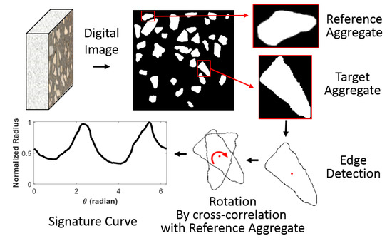
Figure 1.
Digital image processing. The captured aggregate images are processed to obtain the signature curve by detecting, scaling, and rotating the edge of each recognized aggregate shape.
2.1. Sample Preparation
The concrete samples were cast with the Portland cement Type I, fly ash Class C, limestone aggregate grading with a granular diameter from 9.525 to 38.1 mm (0.375 to 1.5 in.), and sand with a particle size range from 0.076 to 4.75 mm (0.003 to 0.187 in.). For the concrete mix, we composed a mixture with 385 kg/m3 (650 lb/yd3) of type I cement and a 0.37 water-binder ratio. Well-graded sand and crushed limestone coarse aggregates with the maximum diameter of ¾ were used. The mixture proportions by mass were 1:0.38:2.84:1.72 (binder: water: fine aggregate: coarse aggregate). Class C fly ash was used in the mix design to increase the workability of the concrete. Moreover, for the higher quality of image processing, a charcoal cement color was added to the batch to provide a higher contrast between the aggregates and cement. The samples were cured for seven days in a moisture curing room. The specimen size was selected in conformity with the American Society for Testing and Materials (ASTM) C 78 standard specifying a 15.24 × 15.24 × 50.8 cm (6 × 6 × 20 in) beam. Two beams were cut with 25.4 mm (1 in.) width slices, and each side of the slice was polished to eliminate the saw machine traces from the surface. Moreover, the surfaces were rinsed to wipe off the dust and mud stemming from the saw and polishing procedure to increase the accuracy of aggregate edge detection.
2.2. Image Registration of Concrete Cross-Section
The DIP algorithm is developed to obtain the aggregate shape profile from the concrete cross-section. The aggregate image is obtained from the cross-section of the specimen. Initially, the images were converted to a grayscale image and then converted to a binary image. In the binary image, the paste is shown with black as the logical value of 0, and aggregates are white as the logical value of 1. To filter out noises (e.g., undesired small particles, large sand particles), a non-aggregate area was eliminated by the filler algorithm based on morphological reconstruction [25]. By implementing the image registration algorithm, the aggregates were labeled and stored as separate images. The aggregate sizes were normalized for shape comparison so that the radiuses of all aggregates do not exceed 1. The aggregate edges were detected using the Sobel approximation, as shown in Figure 1, Edge Detection.
As shown in Figure 2, the signature curve presents an alteration of radius over angle to an aggregate edge from its centroid. Our library contains 1064 coarse aggregates obtained from 40 slices of concrete specimens. From these images using the DIP technique elaborated above, the coordinates of the aggregate edges were obtained and later converted to the polar coordinate system. In Figure 2, the signature curve of the aggregates was plotted with a polar radius versus the polar angle of the aggregate. Figure 2b shows the signature curve of an aggregate illustrated in Figure 2a, which depicts the alteration of the aggregate radius along the aggregate edges at different angles. It can be implied from the curves that the peaks and troughs are the convexity and concavity of the aggregates.
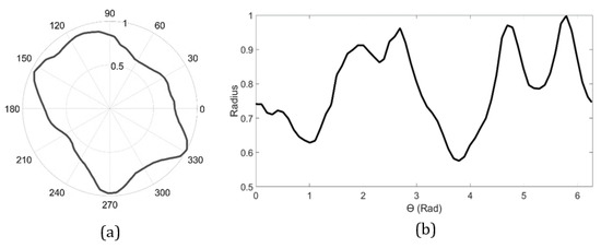
Figure 2.
Representations of an aggregate shape using (a) a polar curve and (b) a signature curve.
2.3. Orientation Matching
The signature curve can be obtained after aggregate degrees are detected. However, the signature curve without the orientation matching process cannot be identified and processed to the statistical analysis due to the phase change. Aggregates with identical orientation empower the statistical analysis to determine the similarity of signature curves. We align aggregates to match the orientation of a reference aggregate by employing the cross-correlation [26]. The cross-correlation between two aggregates and are defined by their corresponding signature curves and , where is the polar angle. Suppose is a reference aggregate whose orientation is fixed. The cross-correlation of and being rotated by in clockwise direction, is given by
Then, the best rotation angle of aggregate is a value such that minimizes this cross-correlation. The first aggregate in the library is usually chosen as the reference aggregate. We calculate the best rotation angles for each aggregate and rotate them accordingly. From now on, we use to refer to a signature curve of the -th aggregate after being optimally rotated.
3. Statistical Methodologies in IFAM
The obtained signature curves from the real aggregate shape are processed to create RSAM, as briefly described in Figure 3. The details of the statistical functional mixture model, RSAM generation technique, are described in this section.
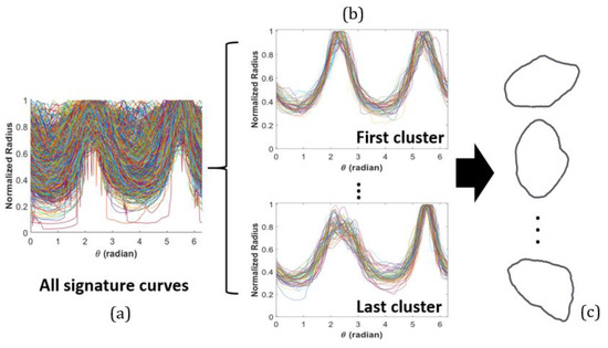
Figure 3.
Conceptual process of image analysis and functional data clustering for random shape aggregate models (IFAM). Different colors are used to visually distinguish each curve, and they contain no meaningful information about the curve profile: (a) all signature curves obtained by digital image processing (DIP), (b) functional mixture model to identify clusters of the curves and (c) simulation of signature curves and back-transformation to aggregate shapes.
3.1. Functional Mixture Models
To establish a model that can represent all aggregates shapes, a single probability model is not appropriate. The broad spectrum of aggregate shapes gives a complex multi-modal distribution, which cannot be well approximated using the single probability model. To overcome this challenge, a functional mixture model is adopted. The model can identify homogeneous groups of prevalent shapes by doing functional-clustering of the signature curves. The mixture model is trained using the signature curves acquired through the DIP process, and tuning parameters are determined by a data-driven way. This model-based approach allows users to generate realistic aggregates with a low computational burden. The proposed method assumes the -th signature curve is a noised observation of the original signal, through the model:
where the noise term are assumed to be independent of . To recover from its noised counterpart, the curves are assumed to have the functional representation based on a finite basis of functions. Let denote the -th basis function and denote the basis coefficient for in its functional representation:
where denotes the number of bases and .
Ramsay et al. have advised choosing the basis according to the nature of the functional data [27]. Because the Fourier bases are periodic, they are the best suitable for describing signature curves, which has a period of . Hence, the Fourier basis is chosen to represent the functional form of signature curves. The Fourier basis is a set of sine and cosine functions of increasing frequency, which is provided by the Fourier series; that is,
for . The number of bases, is odd.
We employ the functional mixture model [28], which models the data into a discriminative functional subspace. The model chooses the latent subspace, which maximizes the separation between the groups. The model takes curves represented by a finite basis function as inputs and gives the posterior probabilities that a curve belongs to each cluster as outputs. This model enables us to cluster aggregate shapes into homogeneous groups. Let denote the unknown class membership of the -th signature curve. The basis coefficient is assumed to have a mixture of multivariate Gaussians:
where is the mixture proportion; is a Gaussian density with mean and covariance , , and are mean and covariance of the latent basis coefficients for cluster , is a matrix mapping the coefficient into the latent subspace; and is the covariance of the error term. The model parameters can be estimated using a funFEM algorithm based on the discriminative functional mixture model, which create the data into a single discriminative functional subspace [28]. We use an R package funFEM for the implementation of the algorithm.
We select p, the number of bases using the generalized cross-validation (GCV) method. The GCV emphasis on the goodness of fit quantified in mean integrated squared error (MISE) relative to the model complexity:
where denote discrete values of to evaluate signature curves. An R package fda.usc [29] can be used to calculate GCV over a search grid to find an optimal value of . The number of clusters, is chosen so as to maximize Bayesian Information Criterion (BIC) of the mixture models over a search grid of .
3.2. Generation of Random Shape Aggregates
In the functional form of signature curves, the aggregate shape is characterized on the basis of coefficient , and its distribution is determined by the functional mixture model in Equation (5). Thus, simulating the basis coefficient is equivalent to simulating the aggregate shape. After estimating the mixture model in Equation (5), we draw samples of basis coefficients from Equation (7) to produce random aggregate shapes across groups as follows:
(1) we use the estimated mixture model,
to draw the basis coefficient ;
(2) The simulated coefficient is plugged-in into the functional representation in Equation (3), so that the simulated signature curve is obtained as follows:
We repeat Steps (1) and (2) until a library of the desired number, of simulated signature curves, is obtained. The curves can be back-transformed to the Cartesian coordinate system to be served as aggregate shapes.
4. Results and Discussions
4.1. RSAM Results
We use R package fda.usc to find a minimum GCV over , and choose . The statistical analysis of the aggregate classifications shows a large between-cluster variation in signature curves. Figure 4 presents BIC values of mixture models over a search grid, . The number of clusters is chosen to be as the optimal value. The number of cluster members for are listed in Table 1. The spaghetti plots of signature curves for each cluster are presented in Figure 5. This figure depicts the noticeable dispersion of signature curves among groups, whereas the within-dispersion of these curves is relatively small.
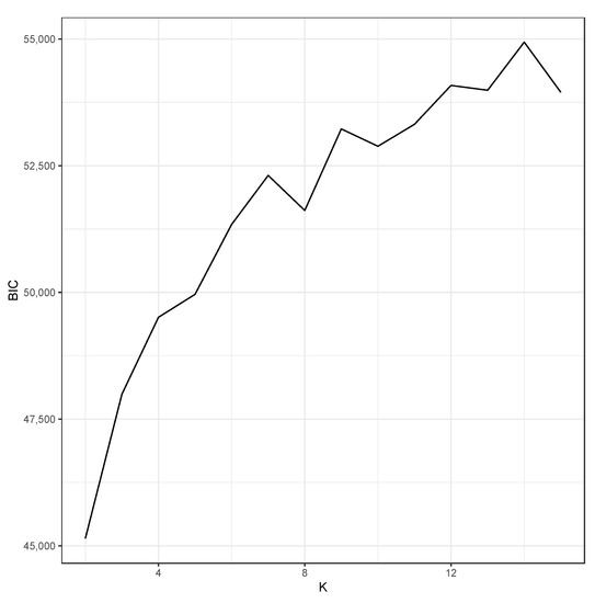
Figure 4.
Bayesian Information Criterion (BIC) calculated for the functional mixture model over K = 2, 3, ···, 15. The BIC is maximized at K = 14.

Table 1.
The number of members in each cluster are obtained using the functional data clustering.
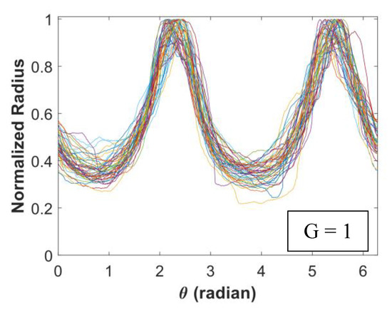
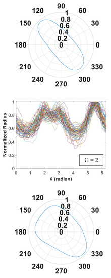
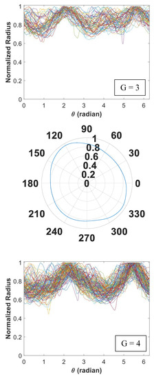
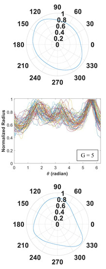
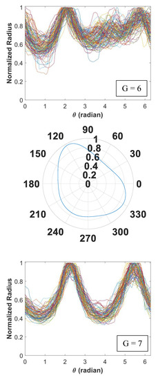
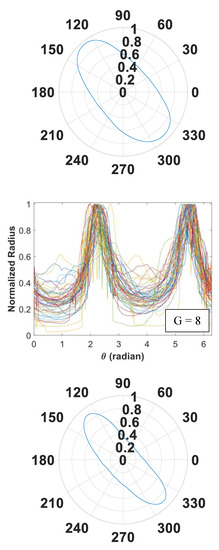
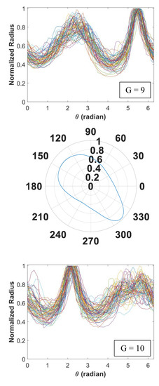
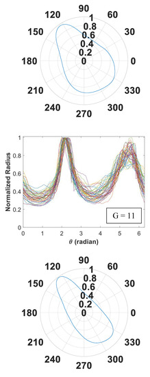
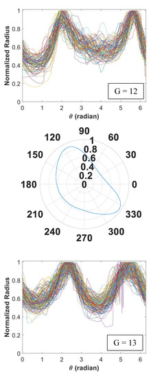
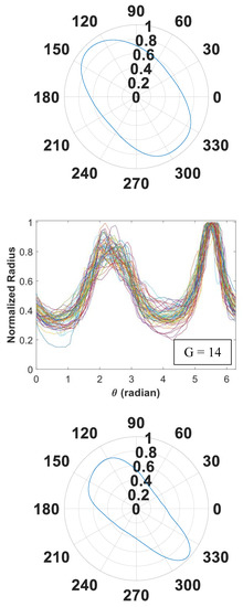
Figure 5.
Signature curves within each cluster are presented in the order by rows (cluster 1 to 14).
In Figure 5, we present 14 identified clusters using individual curves as well as the overall aggregate shapes of each cluster. The overall shapes are obtained from signature curves based on mean basis coefficient values. As shown in these figures, IFAM can explore a broad range of shapes and effectively categorize homogeneous shapes into clusters. We simulated 1064 signature curves and converted them to aggregate shapes. The advantage of IFAM is to learn real aggregate shapes obtained from images of concrete cross-sections. IFAM simulates aggregates within the trained shape profile so that it would generate aggregates with realistic ultrasonic wave reflection, refraction, and mode conversion.
Instead of simulating aggregates across all identified clusters, the simulation using a few selected clusters would be useful when users have interests in particular shapes observed in Figure 5. IFAM allows users to choose to sample signature curves from selected clusters. In fact, users have the power to control the proportion of samples per each cluster. Figure 6 illustrates an example of simulated aggregate shapes. In the figure, one random aggregate from each cluster are sampled, and we aligned them as an array (G = 1,…,14).
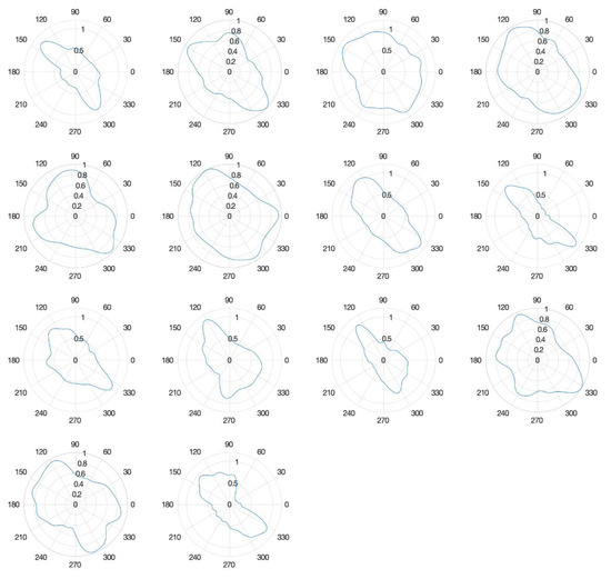
Figure 6.
An example of random aggregate shapes is obtained from Section 3.2. These aggregates are aligned as an array according to the cluster number (G) they belong to: clusters 1 to 4 (top row), 5 to 8 (2nd row), 9 to 12 (3rd row), and 13 to 14 (last row).
4.2. Assessment of IFAM
The performance of IFAM needs to be demonstrated by a comparison of simulated and observed libraries of aggregates. The main goal of RSAM is to generate aggregates that closely follow the observed shape profile. For this reason, such comparison has to be performed at a library level, not at an individual signature curve level. We develop a statistical procedure to assess the global similarity between two libraries of signature curves, simulated and observed ones. The discrepancy between the two signature curves can be measured using MISE. The MISE of two signature curves ( and ) is defined as follows:
To assess the overall discrepancy between a simulated signature curve and the set of all observed signature curves , we use to denote a median of these MISEs:
where the superscript indicates IFAM is used to simulate . The distribution of this median depends on the heterogeneity among observed signature curves, as well as the discrepancy between the simulated signature curve and observed ones. Since our main interest is to determine the discrepancy, we need to establish a reference distribution of the median to take the heterogeneity into account. Roughly speaking, this can be done by calculating the median based on signature curves with zero discrepancies. That is, we use observed signature curves instead of simulated ones. To establish the reference distribution of the overall discrepancy, we use to denote the median of MISEs between an observed signature curve and the set of all observed ones :
Distribution of this median is served as a baseline for . Namely, distributions of and are expected to be similar when the simulated library is similar to the observed library. For comparison, we implement Du and Sun’s method [21] to generate simulated curves, , and calculate as follows:
Their algorithm does not utilize the observed library to generate aggregates. Thus, we expect their simulated signature curve would produce a highly dissimilar distribution of compared to the reference. Boxplots of log M-values for reference, IFAM, and Du and Sun are presented in Figure 7. As we can see in the figure, distributions of and are close to each other, which implies that IFAM generates aggregates whose shapes are similar to real ones. In the meanwhile, the Du and Sun’s method fails to generate aggregates similar to real ones.
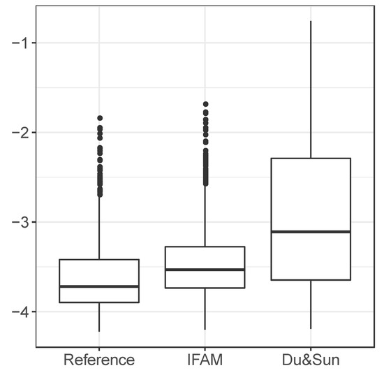
Figure 7.
Boxplots of log M-values obtained from a reference library, simulated aggregates using IFAM and Du and Sun’s method.
5. Conclusions
The model-based RSAM has been developed based on aggregate data obtained using the digital image processing technique. The proposed method uses the functional data clustering to categorize aggregates into homogeneous shape groups. Thus, IFAM randomly generates shapes while it preserves an overall shape pattern within each group. We demonstrate the effectiveness of IFAM over an existing method using the discrepancy between simulated and observed signature curves.
- (1)
- IFAM utilizes a data-driven approach to learn real aggregate shapes. Our flexible learning framework enables us to simulate aggregate shapes close to real ones. Thus, the proposed method is more appropriate for the scattering wave propagation application.
- (2)
- IFAM has the advantage of image processing real aggregates and, therefore, contains the coarse aggregate characteristics such as concavity and irregularities. Unlike other approaches, IFAM is easy to use. We provide data-driven procedures to choose tuning parameters such as the number of bases and the number of clusters in our pipeline so that users do not need to choose these values. Also, the functional mixture model can be trained with a low computational burden. Once the model is trained, users can simulate thousands of aggregates in a few seconds.
- (3)
- The IFAM can be used for concrete structure simulations, especially when the crack propagation pattern is crucially important. Moreover, this technique is essentially useful for understanding wave propagation where the microcrack or crack distribution, including aggrege surrounding environment (i.e., in the vicinity of the interfacial transition zone), and understand that the aggregate shape plays an integral role in wave reflection and refraction.
- (4)
- For future research, we plan to establish a model for the spatial pattern of aggregate shapes, which will enable us to carry out the random placement of the generated aggregates into the sample domain. Also, we plan to extend IFAM for 3D aggregate simulation, which will be served as a research tool for the direction of wave scattering in wave propagation simulation studies.
Author Contributions
Study conception and design: J.Y. and S.H.; data collection: A.D.T.; analysis and interpretation of results: J.Y., S.H., S.K., and A.D.T.; draft manuscript preparation: J.Y., S.K., A.D.T., and S.H.; acquired the funding, supervised the study: S.H. All authors reviewed the results and approved the final version of the manuscript. All authors have read and agreed to the published version of the manuscript.
Funding
This research was supported by the U.S. Department of Transportation, Tran-SET, under grant number 20STUTA26.
Conflicts of Interest
The authors declare no conflict of interest.
References
- Michaels, J.E.; Member, S.; Michaels, T.E.; Member, S. Detection of Structural Damage from the Local Temporal Coherence of Diffuse Ultrasonic Signals. IEEE Trans. Ultrason. Ferroelectr. Freq. Control 2005, 52, 1769–1782. [Google Scholar] [CrossRef] [PubMed]
- Jhang, K.Y. Non-linear ultrasonic techniques for non-destructive assessment of micro damage in material: A Review. Int. J. Precis. Eng. Manuf. 2009, 10, 123–135. [Google Scholar] [CrossRef]
- Ham, S.; Song, H.; Oelze, M.L.; Popovics, J.S. A contactless ultrasonic surface wave approach to characterize distributed cracking damage in concrete. Ultrasonics 2017, 75, 46–57. [Google Scholar] [CrossRef]
- Planès, T.; Larose, E. A review of ultrasonic Coda Wave Interferometry in concrete. Cem. Concr. Res. 2013, 53, 248–255. [Google Scholar] [CrossRef]
- Ren, W.; Yang, Z.; Sharma, R.; Zhang, C.; Withers, P.J. Two-dimensional X-ray CT image based meso-scale fracture modelling of concrete. Eng. Fract. Mech. 2015, 133, 24–39. [Google Scholar] [CrossRef]
- Thilakarathna, P.S.M.; Kristombu Baduge, K.S.; Mendis, P.; Vimonsatit, V.; Lee, H. Mesoscale modelling of concrete—A review of geometry generation, placing algorithms, constitutive relations and applications. Eng. Fract. Mech. 2020, 231, 106974. [Google Scholar] [CrossRef]
- Rodrigues, E.A.; Manzoli, O.L.; Bitencourt, L.A.G., Jr.; Bittencourt, T.N. 2D mesoscale model for concrete based on the use of interface element with a high aspect ratio. Int. J. Solids Struct. 2016, 94–95, 112–124. [Google Scholar] [CrossRef]
- Wang, Z.M.; Kwan, A.K.H.; Chan, H.C. Mesoscopic study of concrete I: Generation of random aggregate structure and finite element mesh. Comput. Struct. 1999, 70, 533–544. [Google Scholar] [CrossRef]
- Chengbin, D. Numerical Simulation of Aggregate Shape of Concrete. In Proceedings of the Earth & Space 2006: Engineering, Construction, and Operations in Challenging Environment, Houston, TX, USA, 5–8 March 2006; Volume 188, p. 158. [Google Scholar] [CrossRef]
- Zhang, Z.; Song, X.; Liu, Y.; Wu, D.; Song, C. Three-dimensional mesoscale modelling of concrete composites by using random walking algorithm. Compos. Sci. Technol. 2017, 149, 235–245. [Google Scholar] [CrossRef]
- Wittmann, F.H.; Sadouki, H. Simulation and Analysis of Composite Structures. Mater. Sci. 1985, 68, 239–248. [Google Scholar] [CrossRef]
- Beddow, J.K.; Meloy, T. Testing and Characterization of Powders and Fine Particles; Heyden: London, UK, 1980. [Google Scholar]
- Unger, J.F.; Eckardt, S. Multiscale Modeling of Concrete. Arch. Comput. Methods Eng. 2011, 18, 341–393. [Google Scholar] [CrossRef]
- Zhou, X.Q.; Hao, H. Mesoscale modelling and analysis of damage and fragmentation of concrete slab under contact detonation. Int. J. Impact Eng. 2009, 36, 1315–1326. [Google Scholar] [CrossRef]
- Wriggers, P.; Moftah, S.O. Mesoscale models for concrete: Homogenisation and damage behaviour. Finite Elem. Anal. Des. 2006, 42, 623–636. [Google Scholar] [CrossRef]
- Xie, Z.H.; Guo, Y.C.; Yuan, Q.Z.; Huang, P.Y. Mesoscopic Numerical Computation of Compressive Strength and Damage Mechanism of Rubber Concrete. Adv. Mater. Sci. Eng. 2015, 2015. [Google Scholar] [CrossRef]
- Giorla, A.; Vaitov, M.; Le Pape, Y.; Temberk, P. Meso-scale modeling of irradiated concrete in test reactor. Nucl. Eng. Des. 2015, 295, 59–73. [Google Scholar] [CrossRef]
- Xu, W.; Chen, H.; Lv, Z. A 2D elliptical model of random packing for aggregates in concrete. J. Wuhan Univ. Technol. Sci. Ed. 2010, 25, 717–720. [Google Scholar] [CrossRef]
- Häfner, S.; Eckardt, S.; Luther, T.; Könke, C. Mesoscale modeling of concrete: Geometry and numerics. Comput. Struct. 2006, 84, 450–461. [Google Scholar] [CrossRef]
- Zheng, J.J.; Zhou, X.Z.; Wu, Y.F.; Jin, X.Y. A numerical method for the chloride diffusivity in concrete with aggregate shape effect. Constr. Build. Mater. 2012, 31, 151–156. [Google Scholar] [CrossRef]
- Du, C.; Sun, L.; Jiang, S.; Ying, Z. Numerical Simulation of Aggregate Shapes of Two-Dimensional Concrete and Its Applications. J. Aerosp. Eng. 2007, 26, 515–527. [Google Scholar] [CrossRef]
- Xu, W.J.; Hu, L.M.; Gao, W. Random generation of the meso-structure of a soil-rock mixture and its application in the study of the mechanical behavior in a landslide dam. Int. J. Rock Mech. Min. Sci. 2016, 86, 166–178. [Google Scholar] [CrossRef]
- Cao, P.; Jin, F.; Changjun, Z.; Feng, D. Investigation on statistical characteristics of asphalt concrete dynamic moduli with random aggregate distribution model. Constr. Build. Mater. 2017, 148, 723–733. [Google Scholar] [CrossRef]
- Huang, J.; Peng, Q.; Hu, X.; Du, Y. A combined-alpha-shape-implicit-surface approach to generate 3D random concrete mesostructures via digital image processing, spectral representation, and point cloud. Constr. Build. Mater. 2017, 143, 330–365. [Google Scholar] [CrossRef]
- Soille, P. Morphological Image Analysis: Principles and Applications; Springer Science & Business Media: Berlin, German, 1999. [Google Scholar]
- Singer, A.; Buck, J.R.; Daniel, M.M. Computer Explorations in Signals and Systems Using MATLAB, 2nd ed.; Pearson: New Jersey, NJ, USA, 2002. [Google Scholar]
- Ramsay, J.; Hooker, G.; Graves, S. Functional Data Analysis with R and MATLAB; Springer: New York, NY, USA, 2009. [Google Scholar]
- Bouveyron, C.; Côme, E.; Jacques, J. The discriminative functional mixture model for a comparative analysis of bike sharing systems. Ann. Appl. Stat. 2015, 9, 1726–1760. [Google Scholar] [CrossRef]
- Febrero-Bande, M.; de la Fuente, M.O. Statistical Computing in Functional Data Analysis: The R Package fda.usc. J. Stat. Softw. 2012, 51. [Google Scholar] [CrossRef]
Publisher’s Note: MDPI stays neutral with regard to jurisdictional claims in published maps and institutional affiliations. |
© 2020 by the authors. Licensee MDPI, Basel, Switzerland. This article is an open access article distributed under the terms and conditions of the Creative Commons Attribution (CC BY) license (http://creativecommons.org/licenses/by/4.0/).