Group Degree Centrality and Centralization in Networks

Abstract

The importance of individuals and groups in networks is modeled by various centrality measures. Additionally, Freeman’s centralization is a way to normalize any given centrality or group centrality measure, which enables us to compare individuals or groups from different networks. In this paper, we focus on degree-based measures of group centrality and centralization. We address the following related questions: For a fixed k, which k-subset S of members of G represents the most central group? Among all possible values of k, which is the one for which the corresponding set S is most central? How can we efficiently compute both k and S? To answer these questions, we relate with the well-studied areas of domination and set covers. Using this, we first observe that determining S from the first question is $\mathcal{NP}$-hard. Then, we describe a greedy approximation algorithm which computes centrality values over all group sizes k from 1 to n in linear time, and achieve a group degree centrality value of at least $(1-1/e)(w^{*}-k)$, compared to the optimal value of $w^{*}$. To achieve fast running time, we design a special data structure based on the related directed graph, which we believe is of independent interest.

1. Introduction

In most networks, some vertices are more central than the others. To model this intuitive feeling, centrality indices were introduced. The first mathematical concept of centrality of graphs was introduced almost 150 years ago by Jordan [1]. There are many ways to provide a measure of the relative “importance” of a node in a network, where the different motivations lead to different centrality measures that were developed in several areas of science.

Node centrality. A social network is typically represented as a graph, where individuals are represented as vertices, and the relationships between pairs of individuals as edges. In the paper, we will freely interchange the terms vertex/node and graph/network, without any meaningful difference.

Various vertex-based measures of centrality have been proposed to determine the relative importance of a vertex within a graph. Arguably, the most common branch of centrality indices is based on the distance between the nodes of the network. Some of the standard centrality indices from this branch are degree, betweenness, closeness, and eccentricity. Among other measures of node centrality, a few of the better known in network analysis are: eigenvector centrality, Google PageRank, Katz centrality, Alpha centrality, and others. For detailed definitions and discussions on various centrality indices, we refer the reader to [2,3,4].

Another concept of vertex centrality, the personalization, was introduced in 2003 (see [5]), and is a measure that shows how central an individual is according to a given subset R (group of important people) in a given social network. In 2005, the subgraph centrality [6] was introduced, which characterizes the participation of each node in all subgraphs in a network and is calculated from the spectra of the adjacency matrix of the network. Recently, Bell [7] introduced the concept called the subgroup centrality, where centrality (of one vertex) is calculated only on a restricted set of vertices. The most basic centrality measure is the degree of a vertex, which we study in this paper.

In 1999, Everett and Borgatti [8] introduced the concept of group centrality which enables researchers to answer questions such as, “How central is the engineering department in the informal influence network of this company?” or, “Among middle managers in a given organization, which are more central, men or women?” With these measures, we can also solve the inverse problem: given a network of ties among organization members, how can we form a team that is maximally central? In [8], the authors introduced group centrality for measures of degree, closeness, and betweenness centrality, which we use in this paper. In 2006, another important group centrality measure motivated by the key players problem was introduced (see [9]). In 2011, Miyano et al. [10] discussed the problem of finding the best group for the so-called k-vertex maximum domination problem (or $k-\mathrm{maxVD}$, in short), which in fact corresponds to maximizing the group degree centrality (introduced in 1999 [8]), where the score is further increased by a constant k.

Freeman’s centralization. In his study, Freeman [11] realized that despite all of the vertex-centrality indices defined up to that point, there was a need for a normalization which could measure the relative importance of a given vertex in a network and would be based on any chosen centrality index. Hence, he defined a centralization measure based on normalized variance in vertex centrality of any chosen centrality measure, with an aim to allow a comparison of distinct networks on the basis of their highest vertex-centralization scores. One may also consider his approach as another type of vertex-centrality, which measures the extent to how some vertex in a network stands out from others in terms of a given centrality index. Every centrality measure can have its own centralization measure. In order to calculate centralization for some vertex measure ${\mathcal{M}}_G:V\left(G\right)\to \mathbb{R}$ in a given graph G, we first define

$$\begin{array}{cc}\hfill \forall v\in V\left(G\right),{\mathcal{M}}_0(G,v)& =\sum _{u\in V\left(G\right)}({\mathcal{M}}_G\left(v\right)-{\mathcal{M}}_G\left(u\right)),\mathrm{and}\hfill \\ \hfill {\mathcal{M}}_0\left(G\right)& =max\{{\mathcal{M}}_0(G,v):v\in V\left(G\right)\}.\hfill \end{array}$$

When there is no risk of confusion regarding the network G, we write ${\mathcal{M}}_0\left(v\right)$ instead of ${\mathcal{M}}_0(G,v)$.

In the same paper, Freeman remarked that the centralizations of degree centrality, betweenness centrality, and closeness centrality achieve their maximum if, and only if G is a star. The statement was later proved in detail by Everett, Sinclair, and Dankelmann [12]. In order to compare centralization values of different graphs with possibly different sizes, in the definition of centralization, Freeman used a normalized formula, where the normalizing divisor is based on the theoretically largest centrality variance in any graph from a given class $\mathcal{G}$ of graphs [11]:

$${\mathcal{M}}_1\left(G\right)=\frac{{\mathcal{M}}_0\left(G\right)}{{max}_{H\in \mathcal{G}}{\mathcal{M}}_0\left(H\right)}.$$

Following Freeman’s approach, the group centralization notion was introduced in [13], which brings us to the focus of this paper.

2. Group Degee Centrality and Centralization

Let ${\mathcal{G}}_n$ be the family of all graphs on n vertices, let $G\in {\mathcal{G}}_n$, and let $S\subseteq V\left(G\right)$. According to [8], the group degree centrality is defined as

$${GD}_G\left(S\right)=\left|\bigcup _{v\in S}N\left(v\right)\setminus S\right|,$$

where $N\left(v\right)$ stands for the set of vertices adjacent to v in G. Also observe that introducing an isolated vertex to a group has zero contribution towards its group degree centrality. Such a vertex will never be considered in the optimal group S, unless S already dominates the non-isolated vertices of G. For easier notation, we will thus only consider graphs without isolated vertices. Given a graph G and integer k, let $S_{G,k}^{*}$ be one of the sets from $\left(\genfrac{}{}{0pt}{}{V\left(G\right)}{k}\right)$ that achieves the maximum value of group degree centrality, that is, ${GD}_G\left(S_{G,k}^{*}\right)={max}_{S\in \left(\genfrac{}{}{0pt}{}{V\left(G\right)}{k}\right)}{GD}_G\left(S\right)$. Observe that $S_{G,k}^{*}$ also takes the maximum value for group degree centralization. Whenever the graph G or the value k are known from the context, we omit the subscript from the notations of centrality, centralization, and similarly simplify the optimal group label to $S_k^{*}$.

As defined in [11,13], ${GD}_1(S,G)$ stands for the group degree centralization. Define $k:=\left|S\right|$, and observe

$$\begin{array}{c}\hfill {GD}_1(S,G)=\frac{{\sum }_{S^{\prime }\in \left(\genfrac{}{}{0pt}{}{V\left(G\right)}{k}\right)}\left({GD}_G\left(S\right)-{GD}_G\left(S^{\prime }\right)\right)}{{max}_{H\in {\mathcal{G}}_n}{\sum }_{S^{\prime \prime }\in \left(\genfrac{}{}{0pt}{}{V\left(H\right)}{k}\right)}\left({GD}_H\left(S_k^{*}\right)-{GD}_H\left(S^{\prime \prime }\right)\right)}.\end{array}$$

(1)

According to Freeman [11], the denominator is needed to normalize centralization, and in turn achieve better relative comparison. Indeed, notice that such normalized values will never exceed value 1. Clearly, as we already mentioned, ${GD}_1(S,G)$ is maximized whenever $GD(S,G)$ is maximized, and by Krnc et al. [13] we have that the maximum value of the denominator corresponds to the star graph $S_n$ and a maximizing set $S_k^{*}$ corresponds to any k-set containing the center of the star. 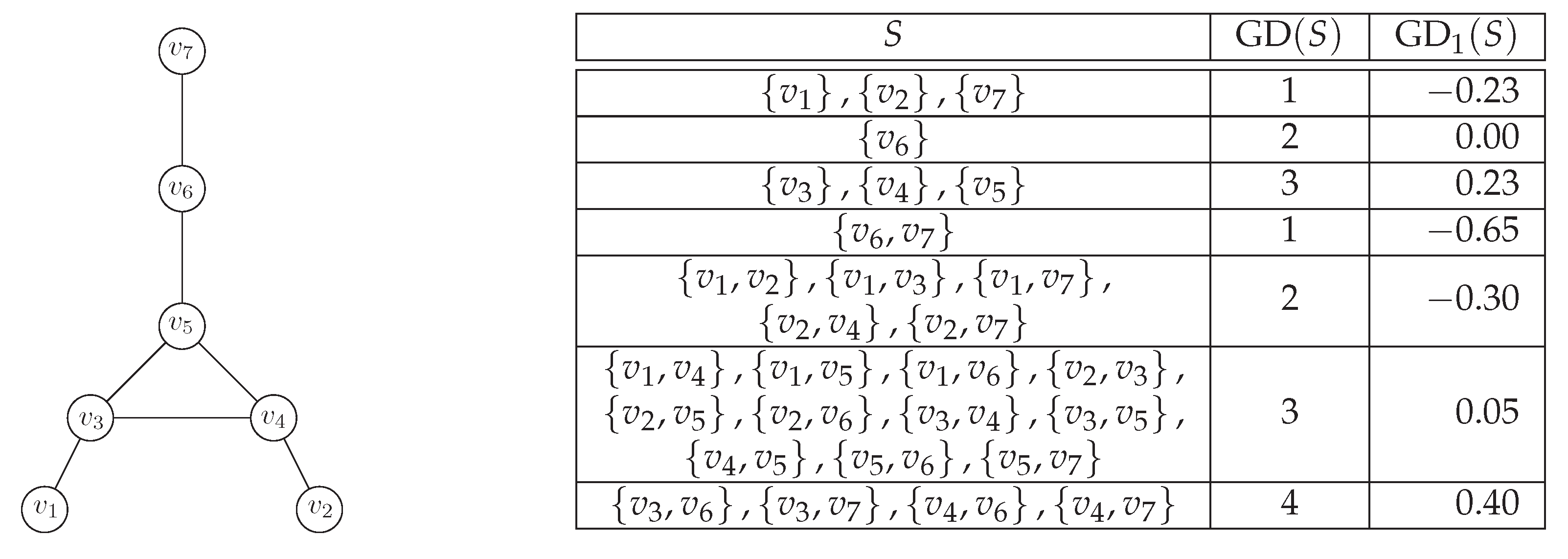In  Figure 1 the group degree centralization is presented of a particular graph.

Given a graph G, define the maximizing group size $k^{*}\left(G\right)$ to be the positive integer, such that

$$\begin{array}{c}\hfill {GD}_G\left(S_{k^{*}\left(G\right)}^{*}\right)=\underset{k\in \left[n\right]}{max}GD(S_k^{*},G),\end{array}$$

where G is known from the context, and we also write $S^{*}:=S_{k^{*}\left(G\right)}^{*}$. Notice that $S^{*}$ achieves the maximum value for group degree centralization as well.

In what follows, we optimize the procedure of calculating the group degree centrality for a given graph and an input integer k. We start by calculating the denominator of the group degree centralization.

Lemma 1.

Let G be a star on n vertices. Then,

$$\sum _{S^{\prime }\in \left(\genfrac{}{}{0pt}{}{V\left(G\right)}{k}\right)}\left(GD\left(S_k^{*}\right)-GD\left(S^{\prime }\right)\right)=(k+1)\left(\genfrac{}{}{0pt}{}{n-1}{k+1}\right).$$

Proof. 

Denote the center of the star by c, partition the sets of $\left(\genfrac{}{}{0pt}{}{V\left(G\right)}{k}\right)$ into parts $P_1$ and $P_2$ depending on whether or not they contain the vertex c as a member, and observe that the group degree centrality of members of these parts equals to $n-k$ and 1, respectively. As ${\sum }_{S^{\prime }\in P_1}\left[GD(S^{*},G)-GD(S^{\prime },G)\right]=0$, the claim follows by:

$$\begin{array}{cc}\hfill \sum _{S^{\prime }\in \left(\genfrac{}{}{0pt}{}{V\left(G\right)}{k}\right)}\left(GD(S^{*},G)-GD(S^{\prime },G)\right)& =\sum _{S^{\prime }\in P_2}\left(GD(S^{*},G)-GD(S^{\prime },G)\right)\hfill \\ \hfill & =\sum _{S^{\prime }\in P_2}(n-k-1)=(k+1)\left(\genfrac{}{}{0pt}{}{n-1}{k+1}\right).\hfill \end{array}$$

 □

In the following proposition, we use a classical graph theoretical approach of double counting to show that the sum ${\sum }_{S^{\prime }\in \left(\genfrac{}{}{0pt}{}{V\left(G\right)}{k}\right)}GD(S^{\prime },G)$ from (1) can be computed efficiently.

Proposition 1.

Let G be a graph on n vertices, and let $k\le n$ be a positive integer. It holds that

$$\sum _{S^{\prime }\in \left(\genfrac{}{}{0pt}{}{V\left(G\right)}{k}\right)}GD(S^{\prime },G)=n·\left(\genfrac{}{}{0pt}{}{n-1}{k}\right)-\sum _{v\in V\left(G\right)}\left(\genfrac{}{}{0pt}{}{n-\mathrm{deg}\left(v\right)-1}{k}\right).$$

In particular, ${\sum }_{S^{\prime }\in \left(\genfrac{}{}{0pt}{}{V\left(G\right)}{k}\right)}GD(S^{\prime },G)$ can be computed in $O\left(n\right)$ time.

Proof. 

For each vertex $v\in V\left(G\right)$, define its contribution $g_k\left(v\right)$ to be the number of k-sets that dominate v, that is,

$$\begin{array}{ccc}\hfill g_k\left(v\right)& =& \left|\left\{X\in \left(\genfrac{}{}{0pt}{}{V\left(G\right)-v}{k}\right);X\cap N\left(v\right)\ne Ø\right\}\right|=\left(\genfrac{}{}{0pt}{}{n-1}{k}\right)-\left(\genfrac{}{}{0pt}{}{n-\mathrm{deg}\left(v\right)-1}{k}\right).\hfill \end{array}$$

By the double counting argument, it follows that

$$\sum _{S^{\prime }\in \left(\genfrac{}{}{0pt}{}{V\left(G\right)}{k}\right)}GD(S^{\prime },G)=\sum _{v\in V\left(G\right)}{g}_k\left(v\right).$$

Thus, we conclude

$$\sum _{S^{\prime }\in \left(\genfrac{}{}{0pt}{}{V\left(G\right)}{k}\right)}GD(S^{\prime },G)=n·\left(\genfrac{}{}{0pt}{}{n-1}{k}\right)-\sum _{v\in V\left(G\right)}\left(\genfrac{}{}{0pt}{}{n-\mathrm{deg}\left(v\right)-1}{k}\right),$$

which can be computed in $O\left(n\right)$ time, traversing all vertices once. □

We join the results from Lemma 1 and Proposition 1 to further develop (1), and claim the following.

Theorem 1.

For a given graph G on n vertices and a group of its vertices S of size k, the group degree centralization can be evaluated as

$$\begin{array}{c}\hfill {GD}_1(S,G)=\frac{\left(\genfrac{}{}{0pt}{}{n}{k}\right)·GD(S,G)+{\sum }_{v\in V\left(G\right)}\left(\genfrac{}{}{0pt}{}{n-\mathrm{deg}\left(v\right)-1}{k}\right)-n·\left(\genfrac{}{}{0pt}{}{n-1}{k}\right)}{\left(k+1\right)·\left(\genfrac{}{}{0pt}{}{n-1}{k+1}\right)},\end{array}$$

(2)

which can be computed in $O\left(n\right)$ time.

It is easy to see that finding $S_k^{*}$ can hence be computed in $O\left(n^{k+1}\right)$, by traversing over all k-tuples and computing group degree centrality at each iteration. However, as k grows, this may not be a feasible approach. As shown below, for an input value of k, determining $S_k^{*}$ is $\mathcal{NP}$-hard. First, recall how the set S of cardinality k is said to be k-dominating whenever

$$\bigcup _{v\in S}N\left(v\right)\cup S=V\left(G\right).$$

Proposition 2.

The problem that determines a set $S_k^{*}$ for a given input graph G and an integer k is $\mathcal{NP}$-hard.

Proof. 

We prove the claim by reducing a well-known $\mathcal{NP}$-problem of determining the existence of a k-dominating set to our problem of finding $S_k^{*}$. Let us assume that there exists a polynomial algorithm for finding a k-set $S_k^{*}\subseteq V\left(G\right)$, such that

$${GD}_G\left(S_k^{*}\right)=\underset{S\in \left(\genfrac{}{}{0pt}{}{V\left(G\right)}{k}\right)}{max}{GD}_G\left(S\right).$$

Now, observe that the existence of a k-dominating set is equivalent to the property

$${GD}_G\left(S_k^{*}\right)=n-k.$$

As group degree centrality of a given fixed set $S_k^{*}$ can be computed in polynomial time $\mathcal{O}\left(nk\right)$, it is clear that the set $S_k^{*}$ provides an answer regarding the existence of a k-dominating set. □

In the last section, we present an efficient algorithm for calculating group degree centrality scores for all group sizes.

3. Greedy Computation of Degree Centrality

By Proposition 2, it is NP-hard to determine the group with the biggest degree centrality. In this section, we present a greedy approach (Algorithm 1) to identify k-sets which are close to achieving the biggest group degree centrality for a given network, for $1\le k\le n$, and describe how one can obtain the corresponding group degree centralization values. Both procedures are described in Algorithms 2 and 3, respectively. We also discuss the corresponding approximability and time complexity.

The greedy algorithm presented here behaves in a natural way:

Algorithm 1 An outline of the greedy algorithm for group degree centrality.

Input: Graph G Output: An ordering S of $V\left(G\right)$ whose prefixes correspond to approximations of sets maximizing group degree centrality. A list L of corresponding group degree centrality values. 1: Let $S=\left[\right]$. 2: Maintain all vertices from $V\left(G\right)\setminus S$ in ordered buckets, labeled by their contribution towards the group degree centrality to set S. 3: Among $V\left(G\right)\setminus S$, append a vertex from a bucket with the biggest label to S. 4: Go to Line 2, unless $V\left(G\right)\setminus S=Ø$. 5: Return S.

In what follows, we describe the important elements of the algorithm. In the next subsection, we present Algorithm 1 in more detail, such as Algorithm 2. The majority of Algorithm 2 deals with step two of the above pseudocode—maintaining all vertices from $V\left(G\right)\setminus S$ in ordered buckets, labeled by their contribution towards the group degree centrality to set S. For efficient implementation of those transitions, we utilised a particular directed graph as a dynamically changing data structure, which enabled us to achieve a linear running time. In the following two subsections, we consider the centralization and complexity, and the approximability analysis as well.

Algorithm 2 Greedy approach to finding a group with the maximum degree centralization.

Input: Graph G. Output: An ordering S of $V\left(G\right)$ whose prefixes correspond to approximations of sets maximizing group degree centrality. A list L of corresponding group degree centrality values. 1: Initialize lists $S=\left(\right)$ and $L=\left(0\right)$. 2: Initialize $G^{\prime }$ as the directed instance of graph G. 3: Partition $V\left(G^{\prime }\right)$ to buckets according to value ${deg}_{G^{\prime }}^{+}\left(v\right)+min(1,{deg}_{G^{\prime }}^{-}\left(v\right))-1$. 4: for all $1\le k\le n$ do                                                                       ▹ Main loop 5:     Append a vertex v from maximal bucket to S. 6:     Append $L[k-1]+{deg}_{G^{\prime }}^{+}\left(v\right)+min(1,{deg}_{G^{\prime }}^{-}\left(v\right))-1$ to L. 7:     for all $u\in N^{+}\left(v\right)$ do 8:         for all $w\in N^{-}\left(u\right)$ do 9:            Remove $(w,u)$ from $G^{\prime }$.                                  ▹ update buckets 10:         end for 11:     end for 12:     Remove v from $G^{\prime }$.                                                 ▹ update buckets 13: end for 14: ReturnS and L.

Algorithm 3 Computing Freeman group degree centralization values.

Input: Graph G. Output: An ordering S of $V\left(G\right)$ whose prefixes correspond to approximations of sets maximizing group degree centrality. A list $L_1$ of corresponding group degree centralization values. 1: Let S and L the lists obtained by Algorithm 2 on input G. 2: Initialize an empty list $L_1=\left(\right)$. 3: for all$1\le k\le n$ do 4:     Compute $\mathcal{S}\leftarrow {\sum }_{S\in \left(\genfrac{}{}{0pt}{}{V\left(G\right)}{k}\right)}GD(S,G)$.                                         ▹ see Proposition 1 5:     Append 2.3 $\frac{\left(\genfrac{}{}{0pt}{}{n}{k}\right)·L\left[k\right]+\mathcal{S}-n·\left(\genfrac{}{}{0pt}{}{n-1}{k}\right)}{\left(k+1\right)·\left(\genfrac{}{}{0pt}{}{n-1}{k+1}\right)}$ to $L_1$.                                                  ▹ see Theorem 1 6: end for 7: Return S and $L_1$.

3.1. The Directed Graph Structure for Implementation

In this subsection, we consider Algorithm 1, which we implement by using a directed graph as a data structure. The corresponding implementation is described as Algorithm 2. The algorithm returns an ordering $S=(v_1,\cdots ,v_n)$ of $V\left(G\right)$, whose prefixes correspond to approximations of sets maximizing group degree centrality, together with a list L of corresponding group degree centrality values. Define $S_k=\{v_1,\cdots ,v_k\}$. We start with an empty list S, and in each iteration, we append a vertex to S which maximizes the contribution towards the current group degree value. The added group degree contributions are then accordingly appended to the list L, and this process is repeated as k increases towards the graph order n.

We describe the state after each iteration k by maintaining a directed graph $G^{\prime }$ on the vertex-set $V\left(G\right)\setminus S_k$, where $(u,v)\in A\left(G^{\prime }\right)$ whenever

• $uv\in E\left(G\right)$, and
• v is not currently dominated by any vertex from S.

At the initialization (i.e., when S is empty), the initial graph $G^{\prime }$ contains all of the edges of G in both directions (line 2). Denote by $G^{\prime }$ our digraph in all iterations of the main loop. For a given vertex $v\notin S_k$, let its contribution towards the group degree centrality be defined as ${GD}_G(S_k\cup \left\{v\right\})-{GD}_G\left(S_k\right)$. Then, the following holds:

Proposition 3.

Let $v\in V\left(G\right)\setminus S_k$, at the beginning of $(k+1)$-th iteration. Then, its contribution equals

$${GD}_G(S_k\cup \left\{v\right\})-{GD}_G\left(S_k\right)={deg}_{G^{\prime }}^{+}\left(v\right)+min(1,{deg}_{G^{\prime }}^{-}\left(v\right))-1.$$

Proof. 

First, note that each out-neighbour of v clearly increments the degree-centrality score by one. Since we assume v was initially not an isolated vertex, it is dominated by $S_k$ whenever ${deg}_{G^{\prime }}^{-}\left(v\right)=0$. In the case when ${deg}^{-}\left(v\right)>0$, that is, when vertex v is not dominated by any other vertex from $S_k$, it is clear that vertex v did not contribute towards the value of $GD\left(S_k\right)$, so we conclude that the contribution simply equals to ${deg}_{G^{\prime }}^{-}\left(v\right)=0$.

To conclude the proof, it remains to consider the case when ${deg}^{-}\left(v\right)=0$. Note that in this case vertex, v was already contributing towards ${\cup }_{u\in S_k}N\left[u\right]$. Since this is not the case after adding v to $S_k$, we have to subtract one from the overall total group degree score. □

It is important to point out that we keep the vertices with the same contribution within the same bucket, and maintain this bucket-structure across all iterations, so it is easy to identify the vertex v, maximizing its contribution. The main loop hence consists of greedily selecting a vertex v which maximizes the group degree centrality contribution, appending it to S (line 5), then appending the corresponding group degree centrality value to L (line 6), and finally updating the directed graph $G^{\prime }$ (lines 7–10). This maintenance of $G^{\prime }$ is done by removing v from $G^{\prime }$, and by removing edges towards all the newly dominated vertices, that is, towards vertices in $N^{+}\left(v\right)$.

3.2. Obtaining Freeman Group Degree Centralization

In order to obtain corresponding values of Freeman’s group degree centralization, we need to normalize group degree centrality scores from Algorithm 2, which is described in Algorithm 3. To determine the sum of all group degree centralities over all k-sets, we apply Proposition 1, for arbitrary value of k. Together with Lemma 1, this suffices to finalize (2) from Theorem 1.

3.3. Complexity and Approximability Analysis

A careful reader may notice a similarity between our greedy approach with the classical greedy appriximation algorithm for MAX COVERAGE or MAX k-VERTEX DOMINATION problems (see [10,14]). While this greedy approach gives an approximation ratio of $1-1/e$ for both mentioned algorithms, any such constant is not attainable for the k-group degree centrality. We now describe the approximability and time complexity of Algorithms 2 and 3, summarised in Theorem 2.

Theorem 2.

Given a graph G on n vertices and m edges, the greedy algorithm for k-group degree centrality over all set sizes $1\le k\le n$ altogether runs in linear time $O(n+m)$ and achieves the k-group degree centrality value of at least $(1-1/e)(w^{*}-k)$, where $w^{*}$ is the maximizing k-group degree centrality of G.

Proof. 

We first deal with the time complexity for Algorithm 2. It is easy to see that the execution of lines outside of the main for-loop takes $O\left(n\right)$ time. For the main for-loop, first note that performing decrementation of a bucket for any vertex takes a constant time. It is also important to observe that any (directed) edge may be identified in a constant time (i.e., lies at up to second neighbourhood of v), and is removed once only. The removal of arbitrary edge $(u,w)$ causes the decrementation of buckets at u, and sometimes also at w. The total number of steps performed by both for-loops in lines 7 and 8 is hence within $\mathsf{\Theta }\left(m\right)$, and so the overall time complexity of Algorithm 2 is $\mathsf{\Theta }\left(m\right)$.

Regarding Algorithm 3, we focus on the complexity of the main for-loop. In particular, line 4 can be computed in $O\left(n\right)$ time, by traversing all vertices and looking at their degrees (see Proposition 1). After this, line 5 is simply a calculation of (2) from Theorem 1, which is performed in $O\left(1\right)$. Thus, the overall time complexity of computing the group degree centralization for all values of k is $O\left(n^2\right)$. Note however that if one is interested in an approximation for a single set-size k, this can be done in $O\left(m\right)$ by executing Algorithm 3 for the specified value of k only.

Let $O_k=\{w_1,w_2,\cdots ,w_k\}\subseteq V\left(G\right)$ be the set maximizing k-group degree centrality, let ${NO}_k={\cup }_{j=1}^{k}N\left[a_j\right]\setminus O_k$, and let $w^{*}=\left|{NO}_k\right|-k$ be the corresponding value of $GD\left(O_k\right)$. For $1\le i\le k$, assume that Algorithm 2 selects vertices $a_i$ in the i-th step, and define

$$\begin{array}{cc}\hfill y_i& =GD\left(\{a_1,\cdots ,a_i\}\right)\hfill \\ \hfill x_i& =y_i-y_{i-1}\hfill \\ \hfill z_i& =w^{*}-y_i,\hfill \end{array}$$

where additionally, we set $y_0=0$ and $z_0=w^{*}$. Notice that $x_i$ denotes the contribution of $a_i$, and $z_i$ tells us how far we are from the optimal value at the i-th step.

Claim.Let $i\le k-1$. Then, $x_{i+1}\ge z_i/k-1$.

Proof. 

It is enough to show that there exists a vertex $x\in O_k$ with at least $z_i/k$ neighbors not in ${\cup }_{j=1}^{i}N\left[a_j\right]$. To this end, observe that at least $z_i$ vertices from ${NO}_k$ are not contained in ${\cup }_{j=1}^{i}N\left[a_j\right]$. Since ${\cup }_{j=1}^{k}N\left[w_j\right]$, there must exist a vertex $w\in O_k$ adjacent to at least $z_i/k$ of those $z_i$ vertices of ${NO}_k\setminus {\cup }_{j=1}^{i}N\left[a_j\right]$.

When our algorithm chooses $a_{i+1}$, the group degree centrality will increase for at least $z_i/k$, and may additionally decrease by 1 in case $w^{*}$ was already dominated before, which concludes the proof of this claim. □

By the above claim, we have

$$\begin{array}{cc}\hfill z_i& \ge \frac{z_i}{k}-1+z_{i+1},\mathrm{i}.\mathrm{e}.,\hfill \\ \hfill z_{i+1}& \le \alpha z_i+1,\hfill \end{array}$$

where $\alpha =1-1/k$. Thus, we get

$$\begin{array}{cc}\hfill z_k& \le {\alpha }^k{z}_0+1+\alpha +\cdots +{\alpha }^{k-1},\mathrm{i}.\mathrm{e}.\hfill \\ \hfill & \le {\alpha }^k{w}^{*}+\frac{1-{\alpha }^k}{1-\alpha },\hfill \end{array}$$

which together with $z_k=w^{*}-y_k$ and ${\alpha }^k\le 1/e$, gives

$$\begin{array}{cc}\hfill y_k& \ge \left(1-{\alpha }^k\right)w^{*}-k\left(1-{\alpha }^k\right)\hfill \\ \hfill & =\left(w^{*}-k\right)\left(1-{\alpha }^k\right)\hfill \\ \hfill & =\left(1-\frac{1}{e}\right)\left(w^{*}-k\right).\hfill \end{array}$$

 □

4. Concluding Remarks and Future Work

With respect to the important branches of the centrality theory, we seek to identify the most central group of nodes in a network, (without fixing the group size in advance). Despite numerous centrality measures, only few are designed to reflect this issue, among them being group centralization measures (see Krnc et al. [13]). We focused on a particular type of group centralization, namely group degree centralization, as it is the simplest one to deal with. The precise calculation of the problem was shown to be infeasible for large networks, and a sub-quadratic approximation algorithm which computes centralization scores over all group sizes was described and analyzed.

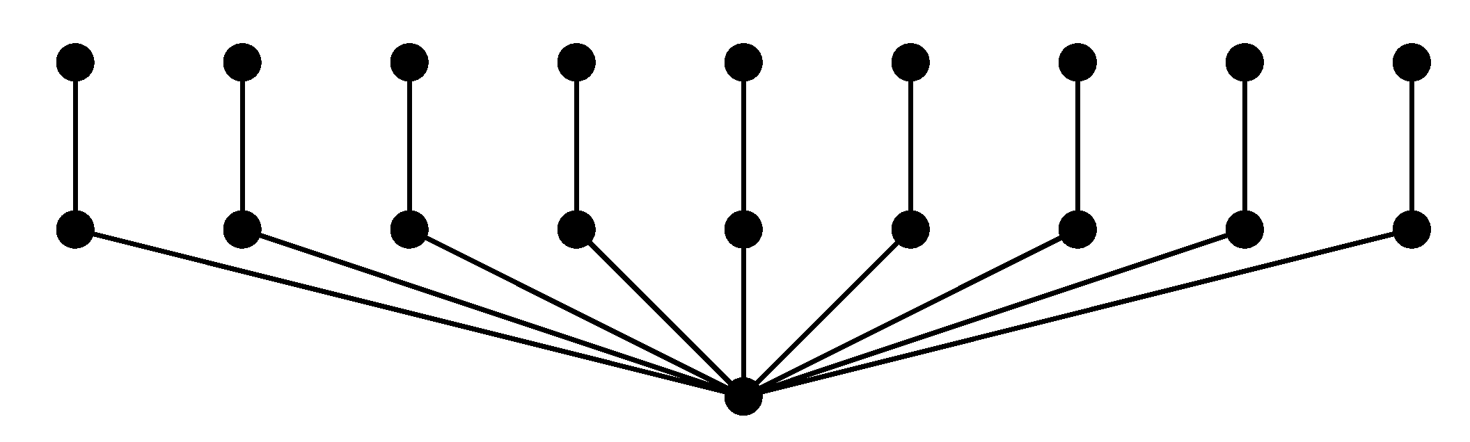
To further justify group degree centralization, it would be most interesting to test the performance of this algorithm on some real-world networks. It is worth noting that Algorithm 2 is not deterministic—indeed, there can be several possibilities in choosing a vertex with the largest contribution. Nevertheless, there exist networks where neither of the possible executions of Algorithm 2 will result in a set which maximizes group degree centrality (for example, see Figure 2).

Additionally, while in this paper we only study the group degree centralization, one should ask similar algorithmic questions for the group centralization of some other centrality indices. One could also consider modifying Freeman’s centralization and consider a different type of normalization for group centrality measures which could preferably be more efficient to calculate.