A Comparative Performance Assessment of Ensemble Learning for Credit Scoring

Abstract
1. Introduction
2. Methodology
2.1. Overviews of Ensemble Learning
2.2. Bagging
Random Forest Algorithm (RF)
2.3. Boosting
2.3.1. AdaBoost
2.3.2. The Related Basic Theory-GBDT
2.3.3. XGBoost Algorithm
2.3.4. LightGBM Algorithm
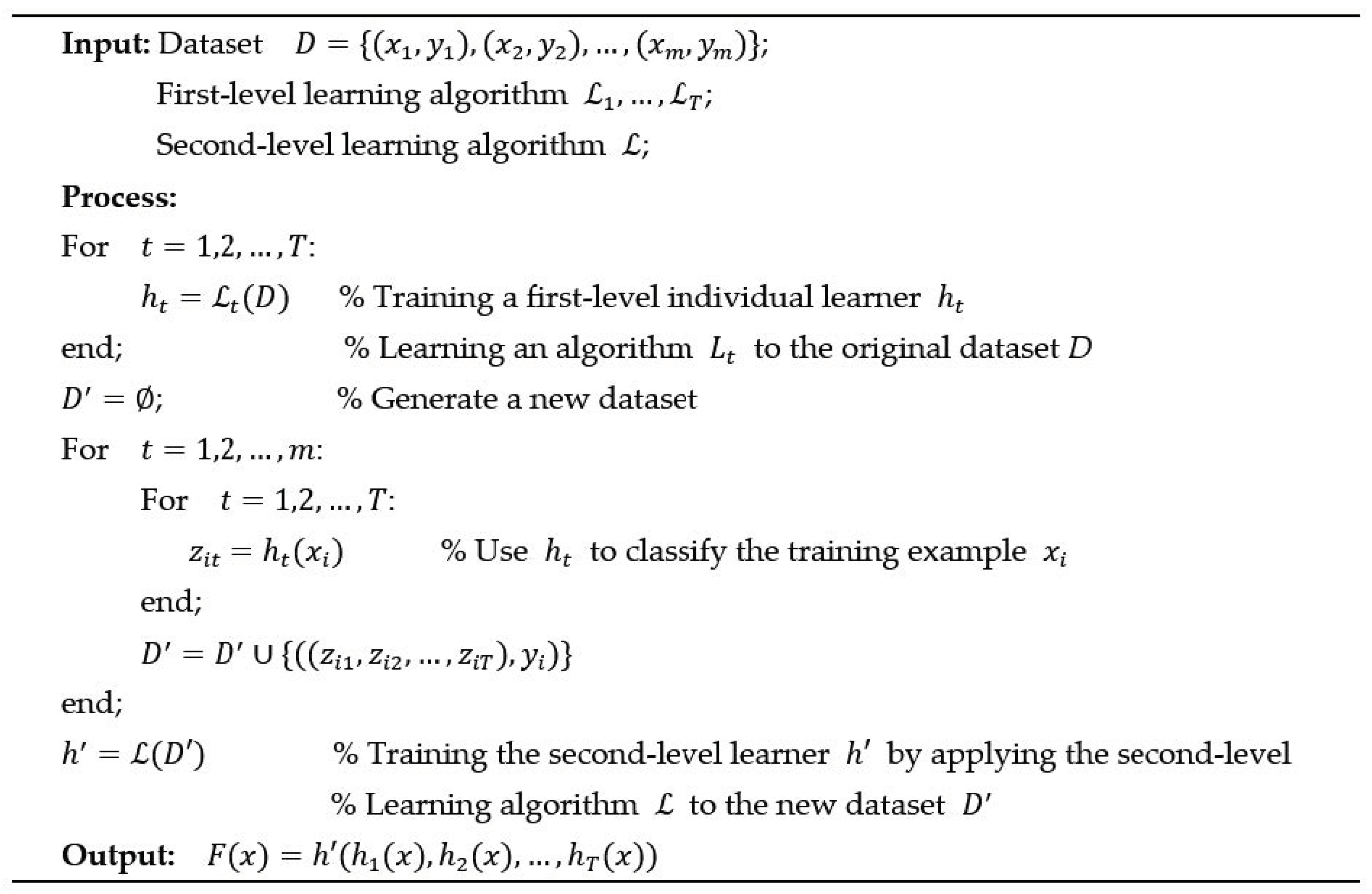
2.4. Stacking
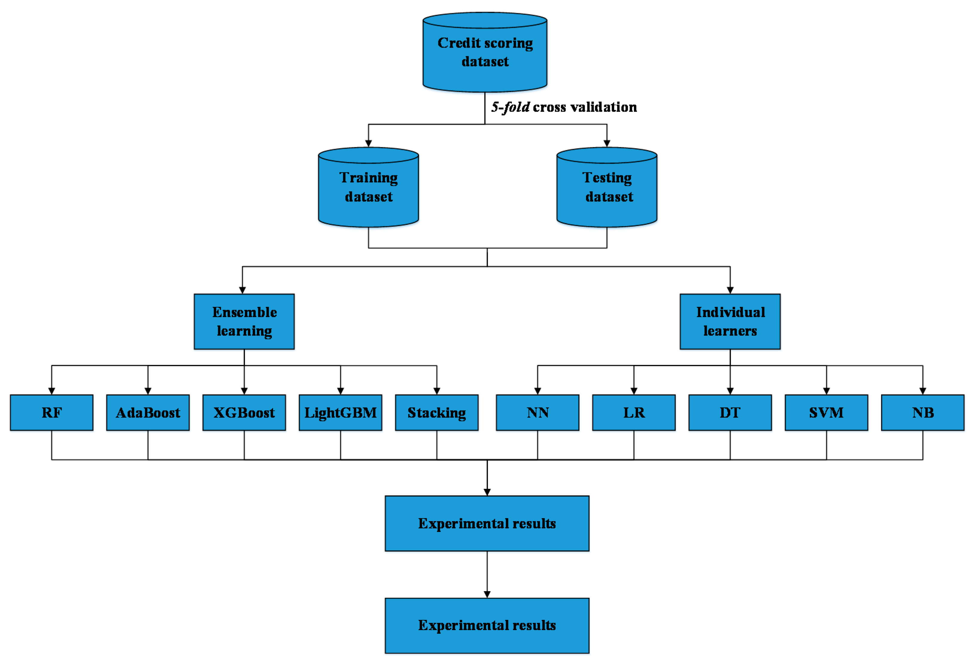
3. Empirical Set-Up
3.1. Data Preparation
3.2. Data Pre-Processing and Feature Selection
3.3. Baseline Classifiers
3.3.1. Neural Network (NN)
3.3.2. Logistic Regression (LR)
3.3.3. Decision Tree (DT)
3.3.4. Naïve Bayes (NB)
3.3.5. Support Vector Machine (SVM)
3.4. Evaluation Criteria
3.5. Hyper-Parameter Tuning
4. Empirical Results
4.1. Classification Results
- (1)
- Compared to traditional individual learners, the ensemble learning has brought a few improvements, except for AdaBoost, this is not consistent with our previous hypothesis.
- (2)
- The reason for the poor performance of AdaBoost may be that the model over-emphasize examples that are noise due to the overfitting of the training data set [33]. Thus RF (Bagging DT) is a relative better choice for credit scoring and this is consistent with prior research.
- (3)
- NN and SVM are both popular credit scoring technique which contain time-consuming training process [45], especially for the data sets of more than 50,000 examples. Thus, they can be excluded in research under the condition of computer hardware equipment is insufficient or not expect to consume too much time, RF, XGBoost, LightGBM, and LR should be the ideal choices for financial institutions in terms of credit scoring and it also provides a reference for future research.
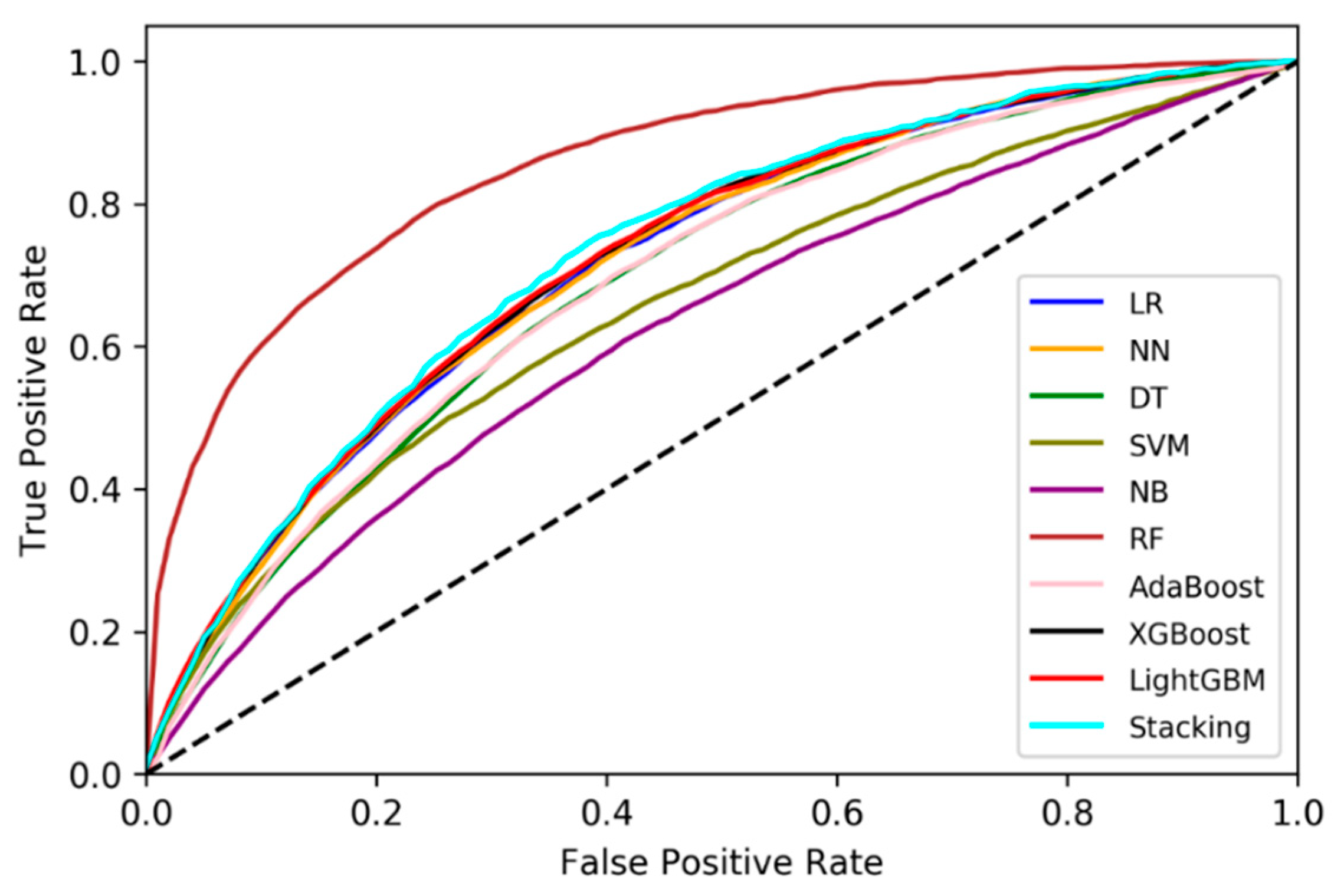
4.2. Receiver Operating Characteristic (ROC) Curve Analysis
5. Conclusions
Author Contributions
Funding
Acknowledgments
Conflicts of Interest
Appendix A. Overview of Variable Definition for Lending Club Dataset

| Variable | Definition | Variable | Definition |
|---|---|---|---|
| Target variable | |||
| Loan status | Whether the borrower is default or not | ||
| Loan characteristic | |||
| Fund amount | The total amount committed to the loan | Initial list status | The initial listing status of the loan. |
| Term | Number of payments on the loan. Values can either be 36 or 60 | collections in 12 months | Number of collections in 12 months excluding medical collections |
| Interest rate | Interest Rate on the loan | Application type | Whether the loan is an individual application or a joint application with two co-borrowers |
| Purpose | Purpose of loan request, 13 purposes included | ||
| Borrowers’ creditworthiness | |||
| Delinquency-2 years | The number of 30+ days past-due incidences of delinquency for the past 2 years | Revolving credit ratio | Total revolving high credit/credit limit |
| Inquires last 6 months | The number of inquiries in past 6 months | Trades last 24 months | Number of trades opened in past 24 months. |
| Open credit lines | The number of open credit lines. | Buying credits | Total open to buy on revolving bankcards |
| Public record | Number of derogatory public records | Ratio of high credit/credit limit | Ratio of total current balance to high credit/credit limit for all bankcard accounts |
| Revolving balance | Total credit revolving balance | Charge-offs last 12 months | Number of charge-offs within 12 months |
| Revolving line utilization rate | The amount of credit the borrower is using relative to all available revolving credit | Past-due amount | The past-due amount owed for the accounts on which the borrower is now delinquent |
| Total credit lines | The total number of credit lines currently | Months bank account opened | Months since oldest bank installment account opened |
| Months old revolving account opened | Months since oldest revolving account opened | Months recent revolving account opened | Months since most recent revolving account opened |
| Months recent account opened | Months since most recent account opened | Mortgage accounts | Number of mortgage accounts |
| Months recent bankcard account | Months since most recent bankcard account opened | Number of overdue accounts | Number of accounts ever 120 or more days past due |
| Active accounts | Number of currently active bankcard accounts | Revolving trades | Number of currently active revolving trades |
| Non-default record | Number of satisfactory bankcard accounts | Number of bankcard | Number of bankcard accounts |
| Installment accounts | Number of installment accounts | Number of open revolving accounts | Number of open revolving accounts |
| Number of revolving accounts | Number of revolving accounts | revolving trades with balance >0 | Number of revolving trades with balance >0 |
| Non-default accounts | Number of satisfactory accounts | Accounts past due last 24 months | Number of accounts 90 or more days past due in last 24 months |
| Accounts opened past 12 months | Number of accounts opened in past 12 months | Percent of non- delinquent trades | Percent of trades never delinquent |
| Percentage of limit bankcard accounts | Percentage of all bankcard accounts > 75% of limit. | Bankruptcies | Number of public record bankruptcies |
| Borrowers’ solvency | |||
| Employment length | Employment length in years. Possible values are between 0 and 10 where 0 means less than one year and 10 means ten or more years. | Verification status | The status of income verification. Verified, source verified or not verified |
| Home ownership | The home ownership status provided by the borrower during registration or obtained from the credit report. Our values are: rent, own, mortgage, other | Address state | The state provided by the borrower in the loan application |
| Annual income | The self-reported annual income provided by the borrower during registration. | DTI | Debt to income ratio |
| Hardship flag | Flags whether or not the borrower is on a hardship plan | ||
References
- World Bank. Global Economic Prospects: Heightened Tensions, Subdued Investment; World Bank Group: Washington, DC, USA, 2019; ISBN 9781464813986. [Google Scholar]
- Huang, C.L.; Chen, M.C.; Wang, C.J. Credit scoring with a data mining approach based on support vector machines. Expert Syst. Appl. 2007, 33, 847–856. [Google Scholar] [CrossRef]
- Hand, D.J.; Henley, W.E. Statistical classification methods in consumer credit scoring: A review. J. R. Stat. Soc. Ser. A Stat. Soc. 1997, 160, 523–541. [Google Scholar] [CrossRef]
- Wang, G.; Hao, J.; Ma, J.; Jiang, H. A comparative assessment of ensemble learning for credit scoring. Expert Syst. Appl. 2011, 38, 223–230. [Google Scholar] [CrossRef]
- Beaver, W.H. Financial ratios as predictors of failure. J. Account. Res. 1966, 4, 71–111. [Google Scholar] [CrossRef]
- Altman, E.I. Financial ratios, discriminant analysis and the prediction of corporate bankruptcy. J. Financ. 1968, 23, 589–609. [Google Scholar] [CrossRef]
- Orgler, Y.E. A credit scoring model for commercial loans. J. Money Credit Bank. 1970, 2, 435–445. [Google Scholar] [CrossRef]
- Grablowsky, B.J.; Talley, W.K. Probit and discriminant functions for classifying credit applicants-a comparison. J. Econ. Bus. 1981, 33, 254–261. [Google Scholar]
- Eisenbeis, R.A. Pitfalls in the application of discriminant analysis in business, finance, and economics. J. Financ. 1977, 32, 875–900. [Google Scholar] [CrossRef]
- Desai, V.S.; Crook, J.N.; Overstreet, G.A., Jr. A comparison of neural networks and linear scoring models in the credit union environment. Eur. J. Oper. Res. 1996, 95, 24–37. [Google Scholar] [CrossRef]
- West, D. Neural network credit scoring models. Comput. Oper. Res. 2000, 27, 1131–1152. [Google Scholar] [CrossRef]
- Atiya, A.F.; Parlos, A.G. New results on recurrent network training: Unifying the algorithms and accelerating convergence. IEEE Trans. Neural Netw. 2000, 11, 697–709. [Google Scholar] [CrossRef] [PubMed]
- Verikas, A.; Gelzinis, A.; Bacauskiene, M. Mining data with random forests: A survey and results of new tests. Pattern Recognit. 2011, 44, 330–349. [Google Scholar] [CrossRef]
- Hsieh, N.-C.; Hung, L.-P. A data driven ensemble classifier for credit scoring analysis. Expert Syst. Appl. 2010, 37, 534–545. [Google Scholar] [CrossRef]
- Ma, X.; Sha, J.; Wang, D.; Yu, Y.; Yang, Q.; Niu, X. Study on a prediction of P2P network loan default based on the machine learning LightGBM and XGboost algorithms according to different high dimensional data cleaning. Electron. Commer. Res. Appl. 2018, 31, 24–39. [Google Scholar] [CrossRef]
- Zhu, Y.; Xie, C.; Wang, G.J.; Yan, X.G. Comparison of individual, ensemble and integrated ensemble machine learning methods to predict China’s SME credit risk in supply chain finance. Neural Comput. Appl. 2017, 28, 41–50. [Google Scholar] [CrossRef]
- Sagi, O.; Rokach, L. Ensemble learning: A survey. Wiley Interdiscip. Rev. Data Min. Knowl. Discov. 2018, 8, 1–18. [Google Scholar] [CrossRef]
- Chen, T.; Guestrin, C. Xgboost: A scalable tree boosting system. In Proceedings of the 22nd ACM SIGKDD International Conference on Knowledge Discovery and Data Mining, San Francisco, CA, USA, 13–17 August 2016; pp. 785–794. [Google Scholar]
- Liang, W.; Luo, S.; Zhao, G.; Wu, H. Predicting hard rock pillar stability using GBDT, XGBoost, and LightGBM algorithms. Mathematics 2020, 8, 765. [Google Scholar] [CrossRef]
- Xia, Y.; Liu, C.; Liu, N. Cost-sensitive boosted tree for loan evaluation in peer-to-peer lending. Electron. Commer. Res. Appl. 2017, 24, 30–49. [Google Scholar] [CrossRef]
- Ala’raj, M.; Abbod, M.F. Classifiers consensus system approach for credit scoring. Knowl.-Based Syst. 2016, 104, 89–105. [Google Scholar] [CrossRef]
- Li, Y.; Chen, W. Entropy method of constructing a combined model for improving loan default prediction: A case study in China. J. Oper. Res. Soc. 2019, 1–11. [Google Scholar] [CrossRef]
- Barboza, F.; Kimura, H.; Altman, E. Machine learning models and bankruptcy prediction. Expert Syst. Appl. 2017, 83, 405–417. [Google Scholar] [CrossRef]
- Alazzam, I.; Alsmadi, I.; Akour, M. Software fault proneness prediction: A comparative study between bagging, boosting, and stacking ensemble and base learner methods. Int. J. Data Anal. Tech. Strateg. 2017, 9, 1. [Google Scholar] [CrossRef]
- Jhaveri, S.; Khedkar, I.; Kantharia, Y.; Jaswal, S. Success prediction using random forest, catboost, xgboost and adaboost for kickstarter campaigns. In Proceedings of the 3rd International Conference Computing Methodologies and Communication (ICCMC), Erode, India, 27–29 March 2019; pp. 1170–1173. [Google Scholar]
- Lessmann, S.; Baesens, B.; Seow, H.-V.; Thomas, L.C. Benchmarking state-of-the-art classification algorithms for credit scoring: An update of research. Eur. J. Oper. Res. 2015, 247, 124–136. [Google Scholar] [CrossRef]
- Brown, I.; Mues, C. An experimental comparison of classification algorithms for imbalanced credit scoring data sets. Expert Syst. Appl. 2012, 39, 3446–3453. [Google Scholar] [CrossRef]
- Saia, R.; Carta, S. Introducing a Vector Space Model to Perform a Proactive Credit Scoring. In Proceedings of the International Joint Conference on Knowledge Discovery, Knowledge Engineering, and Knowledge Management, Porto, Portugal, 9–11 November 2016; Springer: Berlin/Heidelberg, Germany, 2018; pp. 125–148. [Google Scholar]
- Bhattacharyya, S.; Jha, S.; Tharakunnel, K.; Westland, J.C. Data mining for credit card fraud: A comparative study. Decis. Support Syst. 2011, 50, 602–613. [Google Scholar] [CrossRef]
- Wolpert, D.H. Stacked generalization. Neural Netw. 1992, 5, 241–259. [Google Scholar] [CrossRef]
- Breiman, L. Bagging predictors. Mach. Learn. 1996, 24, 123–140. [Google Scholar] [CrossRef]
- Breiman, L. Random forests. Mach. Learn. 2001, 45, 5–32. [Google Scholar] [CrossRef]
- Freund, Y.; Schapire, R.E. Experiments with a New Boosting Algorithm. In Proceedings of the 13th International Conference om Machine Learning, Bari, Italy, 3–6 July 1996; pp. 148–156. [Google Scholar]
- Yuan, X.; Abouelenien, M. A multi-class boosting method for learning from imbalanced data. Int. J. Granul. Comput. Rough Sets Intell. Syst. 2015, 4, 13–29. [Google Scholar] [CrossRef]
- Rao, H.; Shi, X.; Rodrigue, A.K.; Feng, J.; Xia, Y.; Elhoseny, M.; Yuan, X.; Gu, L. Feature selection based on artificial bee colony and gradient boosting decision tree. Appl. Soft Comput. J. 2019, 74, 634–642. [Google Scholar] [CrossRef]
- Ke, G.; Meng, Q.; Finley, T.; Wang, T.; Chen, W.; Ma, W.; Ye, Q.; Liu, T.Y. LightGBM: A highly efficient gradient boosting decision tree. Adv. Neural Inf. Process. Syst. 2017, 2017, 3147–3155. [Google Scholar]
- Witten, I.H.; Frank, E. Data Mining: Practical Machine Learning Tools and Techniques, 2nd ed.; Morgan Kaufmann: San Francisco, CA, USA, 2005. [Google Scholar]
- Xia, Y.; Liu, C.; Da, B.; Xie, F. A novel heterogeneous ensemble credit scoring model based on bstacking approach. Expert Syst. Appl. 2018, 93, 182–199. [Google Scholar] [CrossRef]
- Kennedy, K.; Namee, B.M.; Delany, S.J. Using semi-supervised classifiers for credit scoring. J. Oper. Res. Soc. 2013, 64, 513–529. [Google Scholar] [CrossRef]
- Ala’raj, M.; Abbod, M.F. A new hybrid ensemble credit scoring model based on classifiers consensus system approach. Expert Syst. Appl. 2016, 64, 36–55. [Google Scholar] [CrossRef]
- Louzada, F.; Ara, A.; Fernandes, G.B. Classification methods applied to credit scoring: Systematic review and overall comparison. Surv. Oper. Res. Manag. Sci. 2016, 21, 117–134. [Google Scholar] [CrossRef]
- Xiao, H.; Xiao, Z.; Wang, Y. Ensemble classification based on supervised clustering for credit scoring. Appl. Soft Comput. 2016, 43, 73–86. [Google Scholar] [CrossRef]
- Siddique, K.; Akhtar, Z.; Lee, H.; Kim, W.; Kim, Y. Toward Bulk Synchronous Parallel-Based Machine Learning Techniques for Anomaly Detection in High-Speed Big Data Networks. Symmetry 2017, 9, 197. [Google Scholar] [CrossRef]
- Cortes, C.; Vapnik, V. Support-vector networks. Mach. Learn. 1995, 20, 273–297. [Google Scholar] [CrossRef]
- Abellán, J.; Castellano, J.G. A comparative study on base classifiers in ensemble methods for credit scoring. Expert Syst. Appl. 2017, 73, 1–10. [Google Scholar] [CrossRef]


| Classifiers | Searching Space |
|---|---|
| LR | |
| DT | |
| NN | |
| SVM | |
| RF | , |
| AdaBoost | , |
| XGBoost | , , , |
| LightGBM | , , , , |
| Performance Measure | Traditional Individual Classifier | Ensemble Learning | ||||||||
|---|---|---|---|---|---|---|---|---|---|---|
| NN | SVM | LR | DT | NB | AdaBoost | RF | XGboost | LightGBM | Stacking | |
| ACC | 0.7914 | 0.7919 | 0.7915 | 0.7900 | 0.6828 | 0.7861 | 0.8105 | 0.7947 | 0.7947 | 0.7919 |
| AUC | 0.7201 | 0.6589 | 0.7199 | 0.6952 | 0.6242 | 0.6952 | 0.8580 | 0.7255 | 0.7269 | 0.7337 |
| KS | 0.3299 | 0.2445 | 0.3309 | 0.2969 | 0.1994 | 0.2978 | 0.5507 | 0.3411 | 0.3438 | 0.3643 |
| Brier Score | 0.1497 | 0.1563 | 0.1495 | 0.1536 | 0.2644 | 0.1574 | 0.1260 | 0.1482 | 0.1479 | 0.1476 |
| Classifier | NN | LR | DT | NB | SVM |
|---|---|---|---|---|---|
| Time (s) | 118.7610 | 1.1919 | 2.0758 | 0.2264 | 696.1673 |
| Classifier | RF | AdaBoost | XGBoost | LightGBM | Stacking |
| Time (s) | 0.8949 | 2.7414 | 3.5163 | 1.8071 | 28.5911 |
© 2020 by the authors. Licensee MDPI, Basel, Switzerland. This article is an open access article distributed under the terms and conditions of the Creative Commons Attribution (CC BY) license (http://creativecommons.org/licenses/by/4.0/).
Share and Cite
Li, Y.; Chen, W. A Comparative Performance Assessment of Ensemble Learning for Credit Scoring. Mathematics 2020, 8, 1756. https://doi.org/10.3390/math8101756
Li Y, Chen W. A Comparative Performance Assessment of Ensemble Learning for Credit Scoring. Mathematics. 2020; 8(10):1756. https://doi.org/10.3390/math8101756
Chicago/Turabian StyleLi, Yiheng, and Weidong Chen. 2020. "A Comparative Performance Assessment of Ensemble Learning for Credit Scoring" Mathematics 8, no. 10: 1756. https://doi.org/10.3390/math8101756
APA StyleLi, Y., & Chen, W. (2020). A Comparative Performance Assessment of Ensemble Learning for Credit Scoring. Mathematics, 8(10), 1756. https://doi.org/10.3390/math8101756