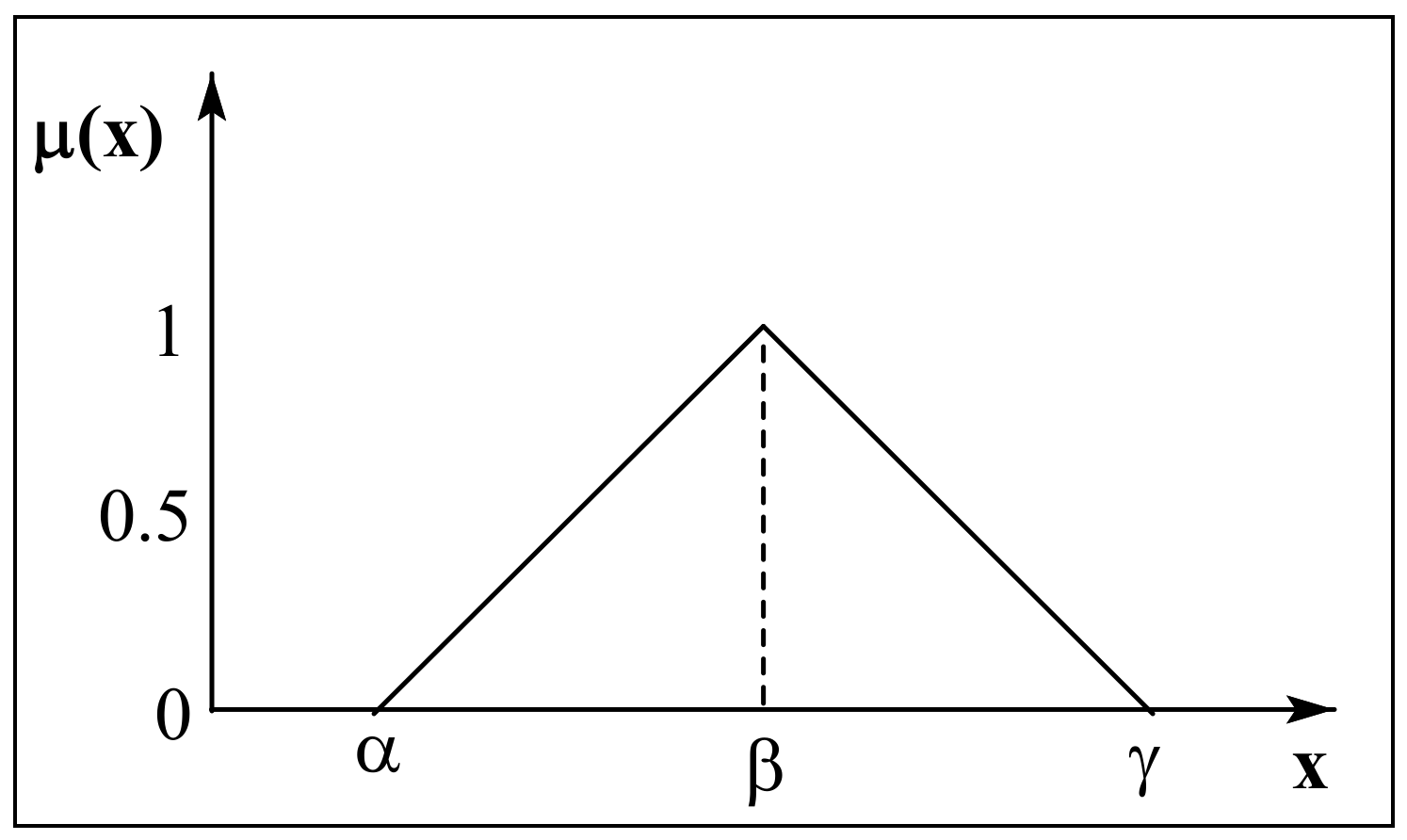
Figure 1.
Triangular Fuzzy Number.
Figure 1.
Triangular Fuzzy Number.
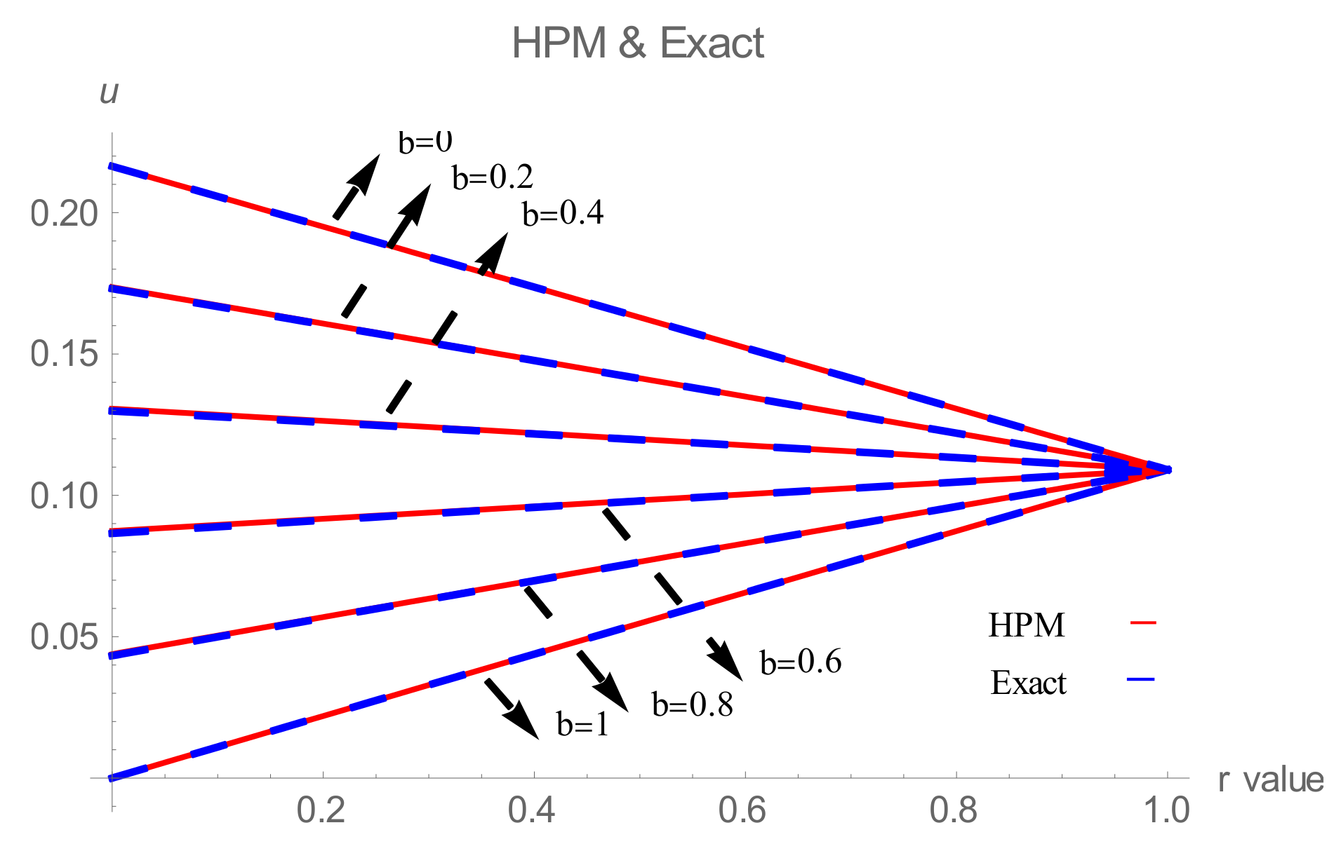
Figure 2.
Comparison of the exact and fifth-order double parametric fuzzy HPM solutions of Equation (24) at for different values of .
Figure 2.
Comparison of the exact and fifth-order double parametric fuzzy HPM solutions of Equation (24) at for different values of .
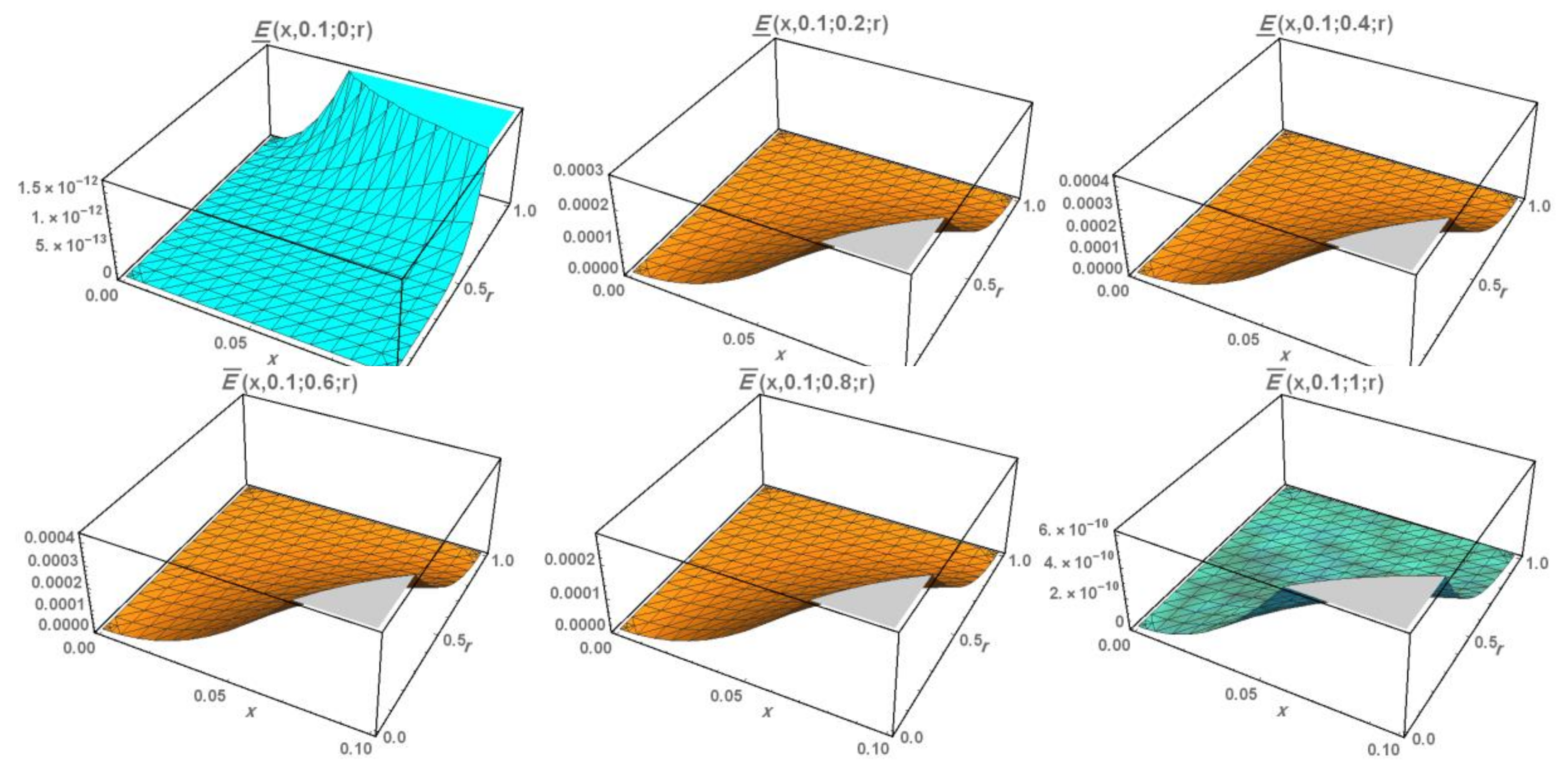
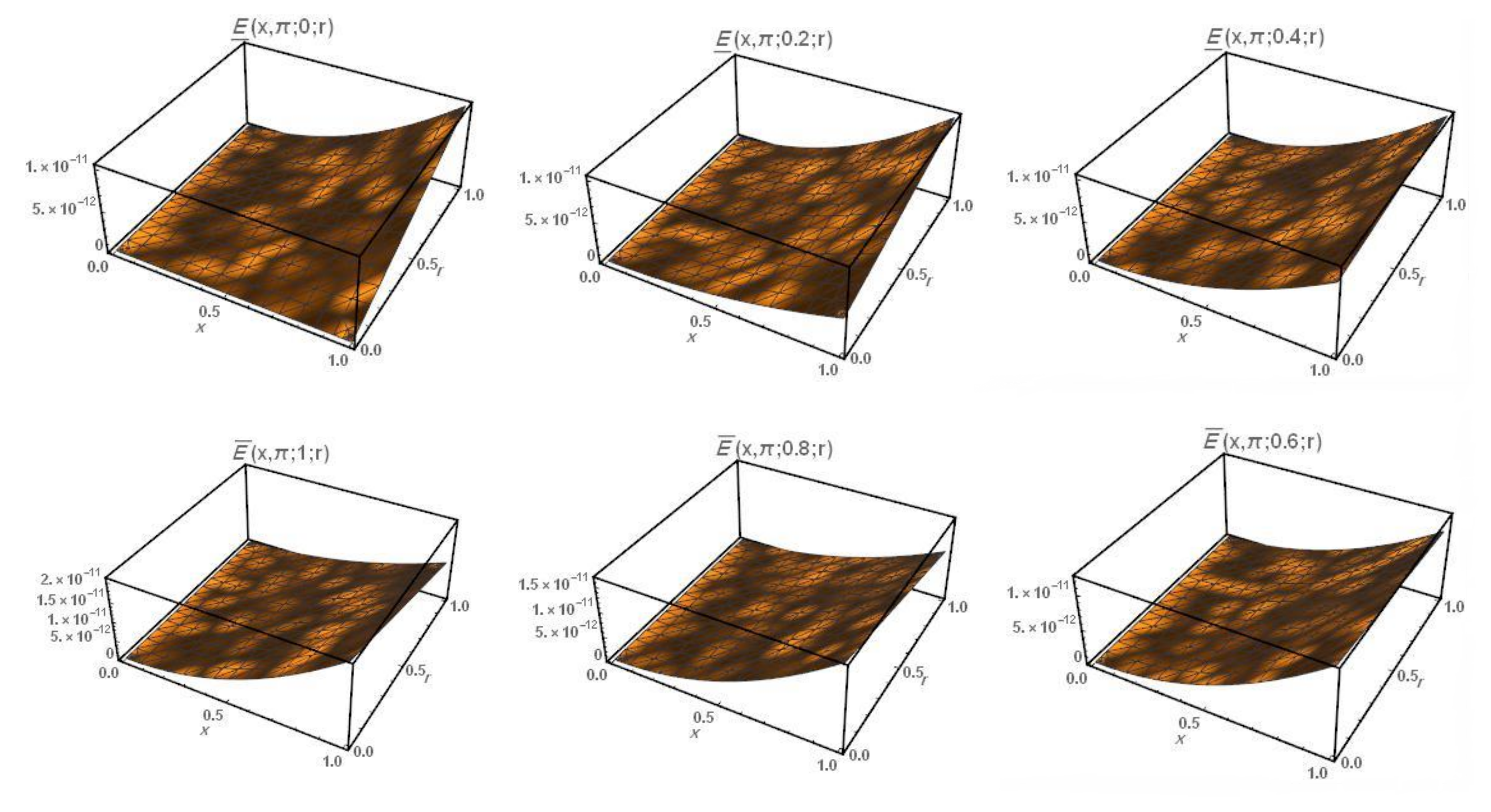
Figure 3.
Accuracy of fifth-order HPM solution at, for all and .
Figure 3.
Accuracy of fifth-order HPM solution at, for all and .
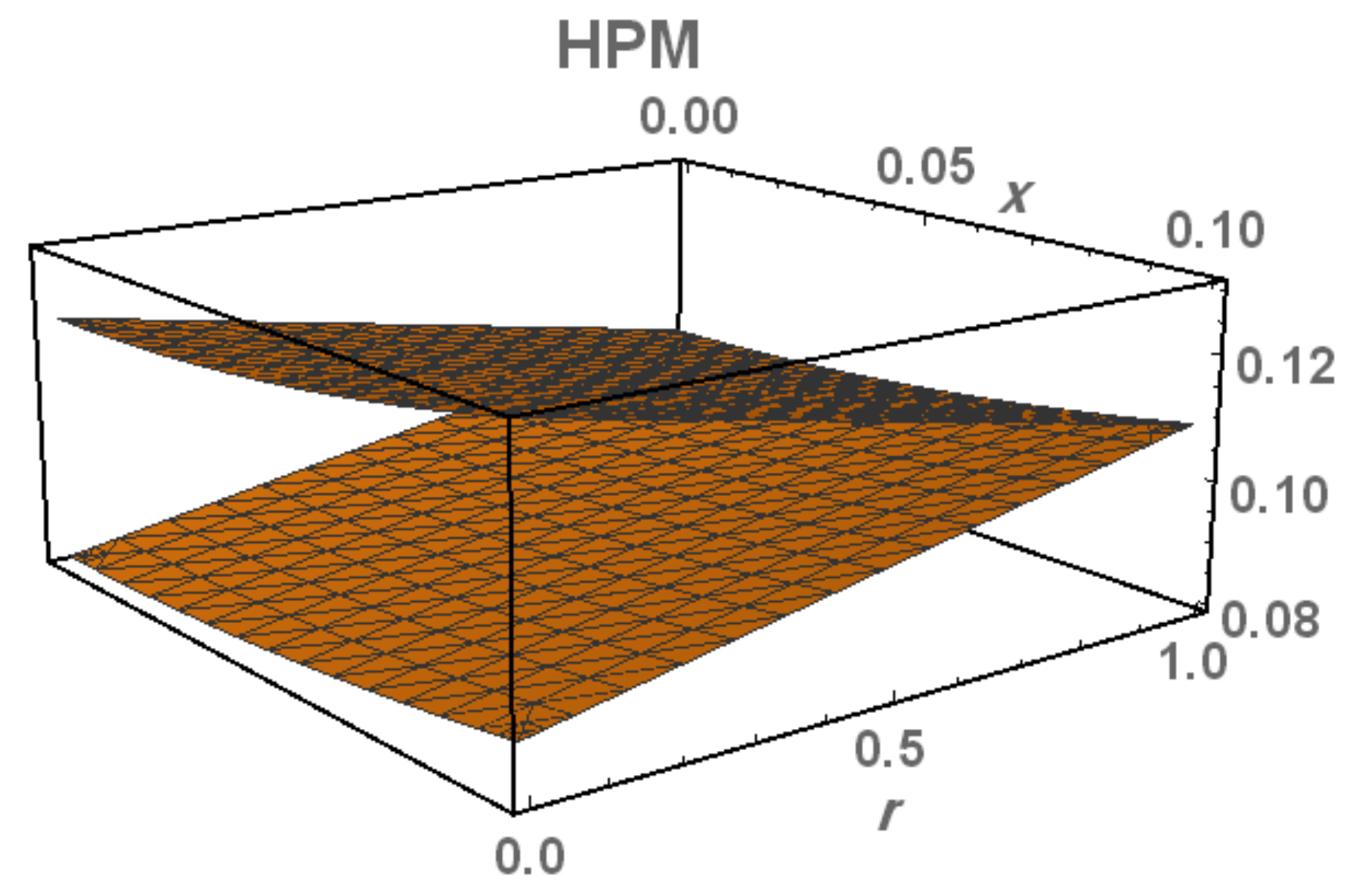
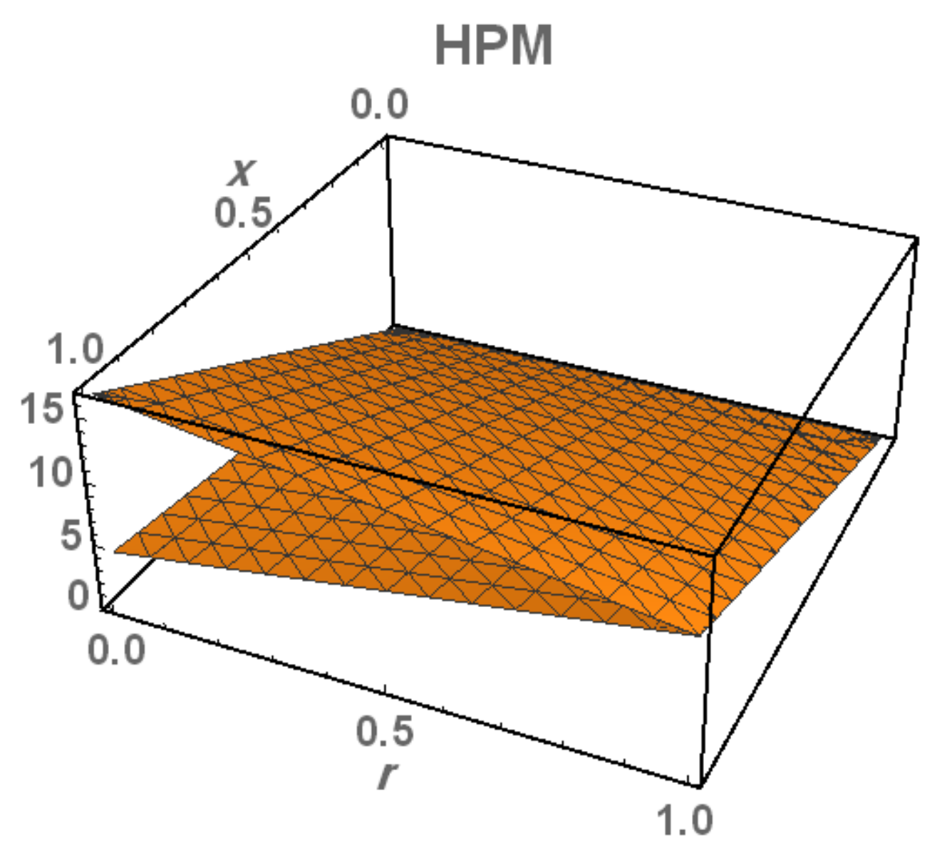
Figure 4.
Solution of fifth-order double parametric fuzzy HPM at , ,1 for all and .
Figure 4.
Solution of fifth-order double parametric fuzzy HPM at , ,1 for all and .
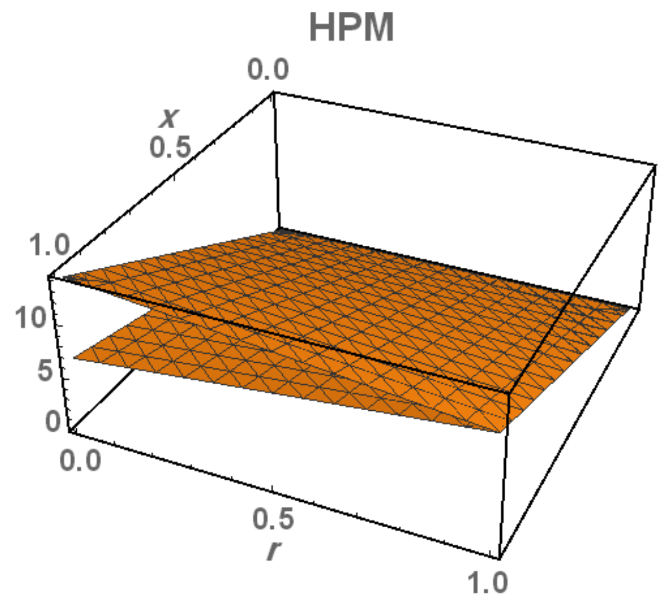
Figure 5.
Solution using the fifth-order double parametric fuzzy HPM at, for all and .
Figure 5.
Solution using the fifth-order double parametric fuzzy HPM at, for all and .
Figure 6.
Solution using fifth-order double parametric fuzzy HPM at , for all and .
Figure 6.
Solution using fifth-order double parametric fuzzy HPM at , for all and .
Figure 7.
Comparison of the exact and tenth-order double parametric fuzzy HPM solutions of Equation (31) at, for different values of .
Figure 7.
Comparison of the exact and tenth-order double parametric fuzzy HPM solutions of Equation (31) at, for different values of .
Figure 8.
Accuracy of the tenth-order double parametric fuzzy HPM solution at , for all and .
Figure 8.
Accuracy of the tenth-order double parametric fuzzy HPM solution at , for all and .
Figure 9.
Solution of the tenth-order double parametric fuzzy HPM at , for all and .
Figure 9.
Solution of the tenth-order double parametric fuzzy HPM at , for all and .
Figure 10.
Solution of the tenth-order double parametric fuzzy HPM at , for all and .
Figure 10.
Solution of the tenth-order double parametric fuzzy HPM at , for all and .
Figure 11.
Solution of the tenth-order double parametric fuzzy HPM at , for all and .
Figure 11.
Solution of the tenth-order double parametric fuzzy HPM at , for all and .
Table 1.
Solution and accuracy of third and fifth order double parametric HPM solutions for Equation (24) at and for all.
Table 1.
Solution and accuracy of third and fifth order double parametric HPM solutions for Equation (24) at and for all.
| | | | | |
|---|
| 0 | 0 | 0 | 0 | 0 | 0 |
| 0.2 | | | | | |
| 0.4 | | | | | |
| 0.6 | | | | | |
| 0.8 | | | | | |
| 1 | | | | | |
Table 2.
Solution and accuracy of third and fifth order double parametric fuzzy HPM solutions for Equation (24) at and for all.
Table 2.
Solution and accuracy of third and fifth order double parametric fuzzy HPM solutions for Equation (24) at and for all.
| | | | | |
|---|
| 0 | | | | | |
| 0.2 | | | | | |
| 0.4 | | | | | |
| 0.6 | | | | | |
| 0.8 | | | | | |
| 1 | | | | | |
Table 3.
Solution and accuracy of third and fifth order double parametric fuzzy HPM solutions for Equation (24) at and for all.
Table 3.
Solution and accuracy of third and fifth order double parametric fuzzy HPM solutions for Equation (24) at and for all.
| | | | | |
|---|
| 0 | | | | | |
| 0.2 | | | | | |
| 0.4 | | | | | |
| 0.6 | | | | | |
| 0.8 | | | | | |
| 1 | | | | | |
Table 4.
Solution and accuracy of third and fifth order double parametric fuzzy HPM solutions for Equation (24) at and for all.
Table 4.
Solution and accuracy of third and fifth order double parametric fuzzy HPM solutions for Equation (24) at and for all.
| | | | | |
|---|
| 0 | | | | | |
| 0.2 | | | | | |
| 0.4 | | | | | |
| 0.6 | | | | | |
| 0.8 | | | | | |
| 1 | | | | | |
Table 5.
Solution and accuracy of third and fifth order double parametric fuzzy HPM solutions for Equation (24) at and for all.
Table 5.
Solution and accuracy of third and fifth order double parametric fuzzy HPM solutions for Equation (24) at and for all.
| | | | | |
|---|
| 0 | | | | | |
| 0.2 | | | | | |
| 0.4 | | | | | |
| 0.6 | | | | | |
| 0.8 | | | | | |
| 1 | | | | | |
Table 6.
Solution and accuracy of third and fifth order double parametric fuzzy HPM solutions for Equation (24) at and for all.
Table 6.
Solution and accuracy of third and fifth order double parametric fuzzy HPM solutions for Equation (24) at and for all.
| | | | | |
|---|
| 0 | | | | | |
| 0.2 | | | | | |
| 0.4 | | | | | |
| 0.6 | | | | | |
| 0.8 | | | | | |
| 1 | | | | | |
Table 7.
Solution and accuracy of fifth and tenth order double parametric fuzzy HPM solutions for Equation (32) at and for all.
Table 7.
Solution and accuracy of fifth and tenth order double parametric fuzzy HPM solutions for Equation (32) at and for all.
| | | | | |
|---|
| 0 | | | | 0 | 0 |
| 0.2 | | | | | |
| 0.4 | | | | | |
| 0.6 | | | | | |
| 0.8 | | | | | |
| 1 | | | | | |
Table 8.
Solution and accuracy of fifth and tenth order double parametric fuzzy HPM solutions for Equation (32) at and for all.
Table 8.
Solution and accuracy of fifth and tenth order double parametric fuzzy HPM solutions for Equation (32) at and for all.
| | | | | |
|---|
| 0 | | | | | |
| 0.2 | | | | | |
| 0.4 | | | | | |
| 0.6 | | | | | |
| 0.8 | | | | | |
| 1 | | | | | |
Table 9.
Solution and accuracy of fifth and tenth order double parametric fuzzy HPM solutions for Equation (32) at and for all.
Table 9.
Solution and accuracy of fifth and tenth order double parametric fuzzy HPM solutions for Equation (32) at and for all.
| | | | | |
|---|
| 0 | | | | | |
| 0.2 | | | | | |
| 0.4 | | | | | |
| 0.6 | | | | | |
| 0.8 | | | | | |
| 1 | | | | | |
Table 10.
Solution and accuracy of fifth and tenth order double parametric fuzzy HPM solutions for Equation (32) at and for all.
Table 10.
Solution and accuracy of fifth and tenth order double parametric fuzzy HPM solutions for Equation (32) at and for all.
| | | | | |
|---|
| 0 | | | | | |
| 0.2 | | | | | |
| 0.4 | | | | | |
| 0.6 | | | | | |
| 0.8 | | | | | |
| 1 | | | | | |
Table 11.
Solution and accuracy of fifth and tenth order double parametric fuzzy HPM solutions for Equation (32) at and for all.
Table 11.
Solution and accuracy of fifth and tenth order double parametric fuzzy HPM solutions for Equation (32) at and for all.
| | | | | |
|---|
| 0 | | | | | |
| 0.2 | | | | | |
| 0.4 | | | | | |
| 0.6 | | | | | |
| 0.8 | | | | | |
| 1 | | | | | |
Table 12.
Solution and accuracy of fifth and tenth order double parametric fuzzy HPM solutions for Equation (32) at and for all.
Table 12.
Solution and accuracy of fifth and tenth order double parametric fuzzy HPM solutions for Equation (32) at and for all.
| | | | | |
|---|
| 0 | | | | | |
| 0.2 | | | | | |
| 0.4 | | | | | |
| 0.6 | | | | | |
| 0.8 | | | | | |
| 1 | | | | | |

 ,
, 


