Exploring a Convection–Diffusion–Reaction Model of the Propagation of Forest Fires: Computation of Risk Maps for Heterogeneous Environments

Abstract

The propagation of a forest fire can be described by a convection–diffusion–reaction problem in two spatial dimensions, where the unknowns are the local temperature and the portion of fuel consumed as functions of spatial position and time. This model can be solved numerically in an efficient way by a linearly implicit–explicit (IMEX) method to discretize the convection and nonlinear diffusion terms combined with a Strang-type operator splitting to handle the reaction term. This method is applied to several variants of the model with variable, nonlinear diffusion functions, where it turns out that increasing diffusivity (with respect to a given base case) significantly enlarges the portion of fuel burnt within a given time while choosing an equivalent constant diffusivity or a degenerate one produces comparable results for that quantity. In addition, the effect of spatial heterogeneity as described by a variable topography is studied. The variability of topography influences the local velocity and direction of wind. It is demonstrated how this variability affects the direction and speed of propagation of the wildfire and the location and size of the area of fuel consumed. The possibility to solve the base model efficiently is utilized for the computation of so-called risk maps. Here the risk associated with a given position in a sub-area of the computational domain is quantified by the rapidity of consumption of a given amount of fuel by a fire starting in that position. As a result, we obtain that, in comparison with the planar case and under the same wind conditions, the model predicts a higher risk for those areas where both the variability of topography (as expressed by the gradient of its height function) and the wind velocity are influential. In general, numerical simulations show that in all cases the risk map with for a non-planar topography includes areas with a reduced risk as well as such with an enhanced risk as compared to the planar case.

1. Introduction

It is the purpose of this contribution to apply a recently-developed efficient numerical method [1] for the solution of a wildland fire model [2] to simulate the propagation of a wildfire in various spatially heterogeneous environments. In particular we demonstrate the use of the method for the computation of so-called risk maps that are based on solving the model under systematic variations of the initial focus of wildfire. The governing model is a particular system of convection–diffusion–reaction partial differential equations (PDEs) that is specified in Section 2.

General principles for the design of models of wildland fire are outlined, for instance, in [3,4]. The model employed herein, due to Asensio and Ferragut [2], is described in detail in [1]. Further references to this model and its variants include [5,6,7]. Applications of this model to real-world wildfire scenarios in several specific geographic regions are documented in [4,8,9]. It is also the basis of the spectral algorithm advanced by San Martin and Torres [10,11], but the particular nature of that numerical method is applicable to a constant diffusion coefficient only. An alternative approach to the description of wildfires through partial differential equations, and their numerical solution by explicit methods is provided in [12,13]. These models and simulators are all based on the principles of combustion theory (see, for instance, [14,15]). Under simplifying assumptions one then obtains a fully three-dimensional reaction–diffusion–convection system governed by thermodynamics [16]. Such systems are usually reduced to two horizontal space dimensions based on the consideration that the ratio of height of vegetation with respect to the characteristic size of a forest is small [17]. Thus, although the combustion process is fully turbulent and three-dimensional, most models used for the simulation of wildfire propagation are formulated and eventually solved in two horizontal space dimensions, although some three-dimensional effects, for instance due to variation of topography, are considered. These include, in particular, [1,2,4,5,6,7,8,9,10,11,12,13]. This simplifaction, especially for large terrains, also reflects limitations in computational resources available. In this context we refer to Tables I and II in [10] for an overview on models, their assumptions, and the corresponding computational treatment. Explicit treatments of the vertical propagation of a forest fire (but on domains of limited horizontal extension) include [18,19]; see also the references cited in these works.

The simulation of a wildfire by numerical solution of an initial-boundary value problem for the governing convection–diffusion–reaction model is a well-known challenge [20] due to the presence of a diffusion term and stiff reaction terms. As a consequence of this property, explicit finite difference schemes are usually associated with a stability condition (CFL condition) that enforces very small time steps for moderate to fine spatial discretizations. This restriction can be avoided by implicit–explicit (IMEX) time discretizations that were introduced for the present wildfire model in our previous paper [1]. These methods impose a less restrictive limitation of the time step than explicit methods. This is achieved by carefully distinguishing between stiff and non-stiff occurrence of the vector of unknowns in the spatially-discretized equations, and choosing the time discretization of the respective terms in a corresponding either implicit or explicit fashion. However, IMEX methods are more general than semi-implicit methods and are based on interlacing evaluations of the stages of particular explicit and implicit Runge–Kutta (RK) schemes [21,22]. We refer to [23,24] as the earliest references to IMEX methods in the context of time-dependent partial differential equations and [25,26,27,28,29,30,31,32,33,34,35] for various applications of IMEX-RK schemes.

IMEX schemes can be understood as sophisticated time discretizations to be applied to the spatial discretization of a partial differential equation, that is, to the governing equation semi-discretized (discrete in space, continuous in time) in a so-called method-of-lines formulation. The spatial discretization itself needs to be done separately. To this end, we herein employ a fifth-order weighted essentially non-oscillatory (WENO) finite-difference discretization [36,37,38] of convective terms on Cartesian grids that can also be regarded as a second-order fully conservative finite-volume discretization on these grids. Our preference for this technique with respect to others, such as finite volume schemes with flux limiters (see [36,39,40] for these and many other alternative schemes) stems from our familiarity with it, in particular in the context of convection–diffusion models related to eco-epidemiological problems [30,31] and non-local models of pedestrian flow [32]. In this work, discontinuous solutions may arise due to degenerate diffusion, as well as sharp gradients, that are dealt with in a robust manner by the WENO reconstructions. Articles that use some mathematics, to make the techniques used more plausible, also include [41].

From a scientific point of view, the contribution and novelty of the present paper is threefold. Firstly, we complement the description of an efficient new numerical method (provided in detail in [1]), namely a linearly implicit IMEX time discretization involving Strang-type operator splitting and WENO spatial discretization by additional examples that demonstrate that the method is flexible enough to handle nonlinear or degenerating diffusion functions and variable topographies. Secondly, we obtain some qualitative insight into the predictions made by the underlying wildfire model. Thirdly, it is demonstrated how the availability of an efficient numerical simulation method can be employed to construct wildfire risk maps for portions of a given terrain.

The remainder of the paper is organized as follows. In Section 2 the governing mathematical model is summarized. We only introduce the model in its final, dimensionless form. Detailed derivations of the wildfire model and its ingredients are provided in [1,2,4]. Next, in Section 3 we outline the numerical method. Numerical results are presented in Section 4. Specifically, after introducing preliminaries in Section 4.1, we simulate in Section 4.2 four scenarios (Scenarios 1.1 to 1.4) with different definitions of $K\left(u\right)$. Then, in Section 4.3 we fix the diffusion coefficient $K\left(u\right)$ and evaluate the influence of the topography of the terrain that affects the wind velocity $\mathit{w}$ through its gradient. To this end we simulate Scenarios 2.1 to 2.4 that differ in the topography of the terrain, in particular the steepness of mountains. Then, based on these topographies, we proceed in Section 4.4 with the computation of risk maps, where the specific risk associated with a point or small patch of the computational domain is the smallness of the time needed to burn a determined fixed amount of fuel (here measured as a percentage of the fuel initially available in $\mathsf{\Omega }$) by a wildfire having its initial focus at that position. Some conclusions are collected in Section 5.

2. Summary of the Mathematical Model

The governing model is the system of convection–diffusion–reaction partial differential equations (PDEs)

$$\begin{array}{cc}\hfill \frac{\partial u}{\partial t}+\nabla ·\left(\mathit{w}(\mathit{x},t)u\right)& =\nabla ·\left(K\left(u\right)\nabla u\right)+f(u,v,\mathit{x}),\frac{\partial v}{\partial t}=g(u,v),\hfill \end{array}$$

(1)

where t is time, $\mathit{x}\in \mathsf{\Omega }$ is the spatial variable where the domain $\mathsf{\Omega }\subset {\mathbb{R}}^2$ represents the forest in which the fire may propagate, and $u=u(\mathit{x},t)$ and $v=v(\mathit{x},t)$ are the scalar unknowns. Here u is the non-dimensionalized temperature and v the non-dimensionalized mass fraction of solid fuel. Moreover, $K=K\left(u\right)$ is a given diffusion coefficient, and $\mathit{w}$ is an advection velocity that represents wind speed. The functions $f(u,v,\mathit{x})$ and $g(u,v)$ are the reactive part of the model. (These ingredients will be specified further below.) The complete wildfire model is described by the system (1) along with zero-flux boundary conditions

$$\left(u\mathit{w}-K\left(u\right)\nabla u\right)·\mathit{n}=0,(\mathit{x},t)\in \partial \mathsf{\Omega }\times (0,+\infty ),$$

(2)

where $n$ is the unit normal vector to $\partial \mathsf{\Omega }$, and the initial conditions

$$u(\mathit{x},0)=u_0\left(\mathit{x}\right),v(\mathit{x},0)=v_0\left(\mathit{x}\right),\mathit{x}\in \mathsf{\Omega }.$$

(3)

We here state the model ingredients in final form, based on the assumption that the dimensional rate r of the chemical reaction of fuel and oxidants into products is given by the Arrhenius equation $r=Aexp(-E_{\mathrm{A}}/\left(RU\right))$, where A is a constant, $E_{\mathrm{A}}$ denotes the activation energy, R is the universal gas constant, and U is absolute temperature (values of parameters are specified in Section 4.1). We mention that precise statements of the assumptions involved in the model development are provided in [1,2,4]. In particular, it is assumed that there is always sufficient amount of oxidant provided by air, so that the conservation law for the oxidant can be ignored (as is stated in the Section 2 of [2]).

If a reference ambient temperature $U_{\mathrm{ref}}=U_{\infty }$ and the non-dimensional inverse of the activation energy $\epsilon =R{U}_{\infty }/E_{\mathrm{A}}$ are given, then the non-dimensional temperature is $u=(U-U_{\infty })/\left(\epsilon U_{\infty }\right)$. Furthermore, time t and the spatial coordinates x and y within $\mathit{x}=(\mathit{x},y)$ are understood as dimensionless variables. Here the original dimensional quantities are non-dimensionalized by the time scale $t_0=(\epsilon /\left(q_{\mathrm{react}}A\right))exp(1/\epsilon )$, where $q_{\mathrm{react}}$ is a non-dimensional reaction heat, and the length scale $l_0={(t_{0}k/\left(\rho C\right))}^{1/2}$, where k is thermal conductivity, C is specific heat, and $\rho$ is the density of the fuel.

Next, we assume that the wind velocity $\mathit{w}$ is given by

$$\begin{array}{c}\hfill \mathit{w}(\mathit{x},t)={\mathit{w}}_0(\mathit{x},t)+\nabla \mathcal{T}\left(\mathit{x}\right),\end{array}$$

(4)

where the vector field ${\mathit{w}}_0(\mathit{x},t)$ is a given wind velocity that may depend on spatial position and time (but is considered constant in our numerical experiments), and $\mathcal{T}\left(\mathit{x}\right)$ is the topography of the domain [10,11]. This choice differs from that of [1], where the terrain was assumed flat, and allows us to include spatial heterogeneity.

Furthermore, we assume that spatial propagation of heat occurs through radiation (as described through the Stefan–Boltzmann law) as well as through natural convection. Then the diffusion function $K\left(u\right)$ is given by

$$\begin{array}{cc}\hfill K\left(u\right)& =\kappa {(1+\epsilon u)}^3+1,\hfill \end{array}$$

(5)

where $\kappa =4\sigma \delta U_{\infty }^3/k$. Here $\sigma$ is the Stefan–Boltzmann constant and $\delta$ is the length of the optical path for radiation through the substance. (The particular functional form (5) is the one derived from first principles in [1,2,4]. In particular, it is based on writing the heat flux by radiation (as defined by the Stefan-Boltzmann law) in dimensionless form as

$$\begin{array}{c}\hfill q=\kappa {(1+\epsilon u)}^3\nabla u=\left(K\left(u\right)-1\right)\nabla u.\end{array}$$

However, for illustrative purposes and since our numerical methods are able to handle a wide range of nonlinear and even degenerate diffusion coefficients, we will also consider alternative algebraic expressions, see Section 4.2). The reaction term $f(u,v,\mathit{x})$ is given by

$$\begin{array}{cc}\hfill f(u,v,\mathit{x})& =v\zeta \left(u\right)-\alpha u,\zeta \left(u\right):=c\left(u\right)exp\left(\frac{u}{1+\epsilon u}\right).\hfill \end{array}$$

(6)

Here the function $c\left(u\right)$ indicates the phase change between the endothermic (solid) and the exothermic (gaseous) phase,

$$\begin{array}{c}\hfill c\left(u\right)=\left\{\begin{array}{cc}1\hfill & \mathrm{if}u\ge u_{\mathrm{pc}},\hfill \\ 0\hfill & \mathrm{if}u<u_{\mathrm{pc}},\hfill \end{array}\right.\end{array}$$

(7)

where $u_{\mathrm{pc}}$ is a given non-dimensional phase change temperature, and $\alpha$ denotes a natural convection coefficient. Finally, the function $g(u,v)$ that accounts for fuel consumption takes the form

$$\begin{array}{cc}\hfill g(u,v)& =-\frac{\epsilon v}{q_{\mathrm{react}}}\zeta \left(u\right).\hfill \end{array}$$

(8)

Summarizing, we may collect the model in its final form and relations necessary in the remainder of the paper as follows. The governing partial differential equations are (1) that are solved along with the boundary conditions (2) and the initial condition (3). As for the coefficient functions in (1), the wind velocity $\mathit{w}(\mathit{x},t)$ is specified by (4) (specific choices of the topography function $\mathcal{T}\left(\mathit{x}\right)$ will be introduced in Section 4.3), the diffusion function $K\left(u\right)$ by (5) (alternative formulas will be discussed in Section 4.2), and the reaction term $f(u,v,\mathit{x})$ by (6) and (7). The fuel consumption function $g(u,v)$ is given by (8). Values of the constants involved in $K\left(u\right)$, $f(u,v,\mathit{x})$ and $g(u,v)$ are provided in Section 4.1.

3. Numerical Method

We assume (for simplicity) a quadratic domain $\mathsf{\Omega }={[0,L]}^2$ and denote by $u=u(\mathit{x},t)$ and $v=v(\mathit{x},t)$ the solution of (1). We define a Cartesian grid with nodes ${\mathit{x}}_{\mathit{i}}=(x_i,y_j)$, $i,j=1,\cdots ,M$, with $x_i=y_i=(i-1/2)\Delta x$, $\Delta x=L/M$, and we define the index vector $\mathit{i}=(i,j)\in \mathcal{M}:={\{1,\cdots ,M\}}^2$. The unit vectors ${\mathit{e}}_1=(1,0)$ and ${\mathit{e}}_2=(0,1)$ are used to refer to neighboring grid points, for instance ${\mathit{x}}_{\mathit{i}+{\mathit{e}}_1}=(x_{i+1},y_j)$ and ${\mathit{x}}_{\mathit{i}+{\mathit{e}}_2}=(x_i,y_{j+1})$. We define $\mathit{u}$ as a solution computed at an instant t in the grid points, where ${\mathit{u}}_i\left(t\right)=\mathit{u}({\mathit{x}}_i,t)$, and analogous notation is used for $\mathit{v}$. For simplicity we denote $K_i=K\left({\mathit{u}}_i\right)$. We may then approximate (1), (5)–(8) in semi-discrete form (that is, in discrete in space but continuous in time form) by the system of ordinary differential equations (ODEs)

$$\begin{array}{c}\hfill \mathrm{d}\mathit{u}/\mathrm{d}t=\mathcal{C}\left(\mathit{u}\right)+\mathcal{D}\left(\mathit{u}\right)\mathit{u}-\mathcal{A}\mathit{u}+v\zeta \left(\mathit{u}\right),\mathrm{d}v/\mathrm{d}t=-(\epsilon /q_{\mathrm{react}})v\zeta \left(\mathit{u}\right).\end{array}$$

(9)

Here the terms $\mathcal{C}\left(\mathit{u}\right)$ and $\mathcal{D}\left(\mathit{u}\right)\mathit{u}$ represent the spatial discretizations of the convective and diffusive terms arising in the first PDE in (1). Their entries are given by $\mathcal{C}\left(\mathit{u}\right)={\left(C{\left(\mathit{u}\right)}_i\right)}_{i\in \mathcal{M}}$, $\mathcal{D}\left(\mathit{u}\right)\mathit{u}={\left({\left(D\left(\mathit{u}\right)\mathit{u}\right)}_i\right)}_{i\in \mathcal{M}}$, where

$$\begin{array}{cc}\hfill C{\left(\mathit{u}\right)}_i& =-\sum _{l=1}^2\frac{1}{\Delta x}\left({\widehat{f}}_{\mathit{i}+\frac{1}{2}{\mathit{e}}_l}-{\widehat{f}}_{\mathit{i}-\frac{1}{2}{\mathit{e}}_l}\right),\hfill \\ \hfill {\left(D\left(\mathit{u}\right)\mathit{u}\right)}_{\mathit{i}}& =\sum _{l=1}^2\frac{1}{2\Delta x^2}\left((K_{\mathit{i}}+K_{\mathit{i}-{\mathit{e}}_l}){\mathit{u}}_{\mathit{i}-{\mathit{e}}_l}-(K_{\mathit{i}-{\mathit{e}}_l}+2K_{\mathit{i}}+K_{\mathit{i}+{\mathit{e}}_l}){\mathit{u}}_{\mathit{i}}+(K_{\mathit{i}}+K_{\mathit{i}+{\mathit{e}}_l}){\mathit{u}}_{\mathit{i}+{\mathit{e}}_l}\right),\hfill \end{array}$$

where ${\widehat{f}}_{\mathit{i}+\frac{1}{2}{\mathit{e}}_l}$ is the numerical flux corresponding to the fifth-order WENO spatial discretization of the convective term $\nabla ·\left(\mathit{w}\mathit{u}\right)$ [35]. For the boundary conditions (2), we can apply absorbing or reflective boundary conditions in each dimension by imposing ghost nodes.

To summarize the strategy to convert (9) into a fully discrete method, let us consider first the ODE system that results from (1), (5)–(8) by omitting heat transport and diffusion terms, namely

$$\begin{array}{c}\hfill \mathrm{d}u/\mathrm{d}t=v\zeta \left(u\right),\mathrm{d}v/\mathrm{d}t=-(\epsilon /q_{\mathrm{react}})v\zeta \left(u\right).\end{array}$$

(10)

We discretize (10) implicitly in time for $v$ and explicitly for $\mathit{u}$. The resulting scheme can be written as

$$\begin{array}{c}\hfill {\mathit{u}}^{n+1}={\mathit{u}}^n+\Delta t\zeta \left({\mathit{u}}^n\right)v^{n+1},v^{n+1}=\frac{v^n}{{\displaystyle 1+\Delta t(\epsilon /q_{\mathrm{react}})\zeta \left({\mathit{u}}^n\right)}}.\end{array}$$

(11)

In order to evaluate (11) in each iteration step, we first compute the value of $v^{n+1}$, then this value is used to compute ${\mathit{u}}^{n+1}$. Now, we associate with (11) the solution operator ${\psi }_{\Delta t}$ defined by

$${\psi }_{\Delta t}({\mathit{u}}^n,v^n)=({\mathit{u}}^{n+1},v^{n+1}).$$

The remaining part of the system (9), namely the system of ordinary differential equations

$$\mathrm{d}\mathit{u}/\mathrm{d}t=\mathcal{C}\left(\mathit{u}\right)+\mathcal{D}\left(\mathit{u}\right)\mathit{u}-\mathcal{A}\mathit{u},$$

(12)

is discretized by a linearly implicit IMEX-RK method. Full technical details of this procedure are provided in [1], and are similar to treatments of related convection–diffusion problems [25,26,27,28]. To explain the main idea, let us recall that in principle Runge–Kutta (RK) ODE solvers could be applied to solve (9) numerically. For instance, strong stability preserving (SSP) explicit RK schemes are a popular class of time integrators associated with a favorable stability constraint on the time step $\Delta t$ [25,26,27,28,29,33,34,35]. Alternatively, once could employ implicit–explicit Runge–Kutta (IMEX-RK) methods (see [33,34,35]), for which only the diffusion term is treated implicitly. In this case the stability condition on $\Delta t$ is less restrictive than for explicit discretizations, but a large system of nonlinear algebraic equations must be solved in each time step. This shortcoming of IMEX-RK methods is avoided by the methodology proposed in [25,26] that is based on linearly implicit–explicit RK schemes, and which is applied here to the discretization of (1). The idea is to distinguish the terms arising in (9) between stiff and non-stiff dependence on the solution vectors $\mathit{u}$ and $v$. One then chooses the time discretization by an implicit and an explicit RK scheme for the terms involving stiff and non-stiff dependence, respectively. In the product $\mathcal{D}\left(\mathit{u}\right)\mathit{u}$, the dependence on $\mathit{u}$ within $\mathcal{D}\left(\mathit{u}\right)$ is considered non-stiff, while that of the factor $\mathit{u}$ is considered stiff. On the other hand, in the product $v\zeta \left(\mathit{u}\right)$, the term $\zeta \left(\mathit{u}\right)$ is considered non-stiff, while the term $v$ is considered stiff. Based on this distinction, the resulting linearly implicit IMEX-RK method for (12) is defined by a pair of RK schemes, namely an explicit one (ERK scheme) and a diagonally implicit one (DIRK scheme) that handle the non-stiff and stiff dependencies, respectively, and one alternates between evaluations of the stages of the ERK scheme and solving linear systems to to evaluate those of DIRK scheme. The details of this procedure are outlined in [1], and we employ here the same coefficients, namely the IMEX-RK scheme H-LDIRK3(2,2,2) defined by a pair of particular two-stage ERK and DIRK schemes [25,27]. The resulting discretization of (12) over a time step of length $\Delta t$ can be written as

$$\begin{array}{c}\hfill {\phi }_{\Delta t}({\mathit{u}}^n,v^n)=({\mathit{u}}^{n+1},v^n),\end{array}$$

where ${\mathit{u}}^{n+1}$ is the approximation of (12) by the IMEX-RK method. Then the complete Strang splitting method (cf. [39,42,43]) to solve (9) is formulated as

$$\begin{array}{c}\hfill ({\mathit{u}}^{n+1},v^{n+1})={\psi }_{\Delta t/2}\circ {\phi }_{\Delta t}\circ {\psi }_{\Delta t/2}({\mathit{u}}^n,v^n).\end{array}$$

Once again we refer to [1] for details on the numerical method.

4. Numerical Results

4.1. Preliminaries

The values of parameters used in all examples are the universal gas constant $R=1.987207\mathrm{cal}/\left(\mathrm{K}\mathrm{mol}\right)$, an ambient temperature of $U_{\infty }=303\mathrm{K}$, an activation energy $E_{\mathrm{A}}=20\mathrm{k}\mathrm{cal}/\mathrm{mol}=83.68\mathrm{kJ}/\mathrm{mol}$ which yields $\epsilon =0.02980905\approx 0.03$, and $A={10}^9{\mathrm{s}}^{-1}$ [15]. The mean magnitudes of other constants, for the numerical examples in [2], and which we adopt for our numerical experiments in [1] as well as herein, are

$$\begin{array}{c}\hfill \rho =100\mathrm{kg}{\mathrm{m}}^{-3},C=1\mathrm{kJ}{\mathrm{kg}}^{-1}{\mathrm{K}}^{-1},k=1\mathrm{W}{\mathrm{m}}^{-1}{\mathrm{K}}^{-1}.\end{array}$$

(13)

Furthermore, Asensio and Ferragut [2] chose the heat of combustion H in such a way that one can assume $q_{\mathrm{react}}=1$. Utilizing the parameters (13), we then get

$$\begin{array}{c}\hfill t_0=\frac{0.03}{{10}^9{\mathrm{s}}^{-1}}exp(1/0.03)=8986.8\mathrm{s},l_0={\left(0.089868{\mathrm{m}}^2\right)}^{1/2}=0.2998\mathrm{m}\end{array}$$

(see the formulas in Section 2). In the numerical examples we keep h constant and small, such that $\alpha ={10}^{-3}$. The inverse of the conductivity coefficient is chosen as $\kappa =0.1$, and we choose non-dimensional wind velocities in a different way in each example.

At the moment we do not have access to the specific value of $U_{\mathrm{pc}}$. However, we may estimate the maximal temperature $u_{max}$ that is attainable. To this end, we examine the ODE system (10), meaning

$$\begin{array}{c}\hfill \mathrm{d}\mathit{u}/\mathrm{d}t=-(q_{\mathrm{react}}/\epsilon )\mathrm{d}v/\mathrm{d}t.\end{array}$$

On the other hand, the second equation in (10) implies that $\mathrm{d}v/\mathrm{d}t\le 0$, while $v\left(t\right)\ge 0$ if $v\left(0\right)\ge 0$. Thus we conclude that

$$\begin{array}{c}\hfill u\left(t\right)=-(q_{\mathrm{react}}/\epsilon )v\left(t\right)+(q_{\mathrm{react}}/\epsilon )v\left(0\right)+u\left(0\right)\le (q_{\mathrm{react}}/\epsilon )v\left(0\right)+u\left(0\right)=:u_{max}.\end{array}$$

For instance, assume that at some point in the spatial domain we impose the initial temperature such that $u\left(0\right)=30$, which corresponds to $U=(1+30\epsilon )U_{\infty }=1.9U_{\infty }=570\mathrm{K}$. This assumption implies that $u_{\max }=(1/\epsilon )+30=63.\overline{3}$, or equivalently, a maximum temperature (in absolute value) of $U_{max}=(1+\epsilon u_{max})U_{\infty }=870\mathrm{K}$. In light of this calculation we will choose either $u_{\mathrm{pc}}=0$ or $0<u_{\mathrm{pc}}\le u\left(0\right)<u_{max}$, where $u\left(0\right)$ is the dimensionless temperature at the point where the fire starts.

In all numerical examples (with the exception of the accuracy test, Scenario 2.0) we employed the method introduced as S-LIMEX in [1] and assume a spatial domain $\mathsf{\Omega }={[0,L]}^2$ with $L=200$. The uniform spatial discretization is chosen as $\Delta x=1$, so that the computational domain $\mathsf{\Omega }$ is subdivided into $200\times 200$ cells.

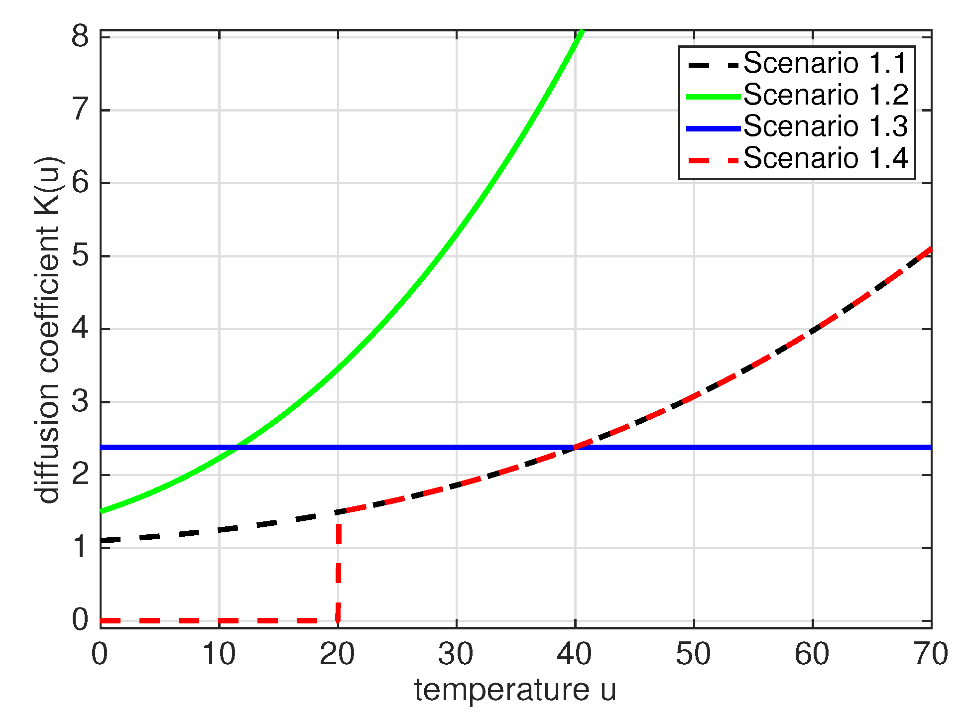
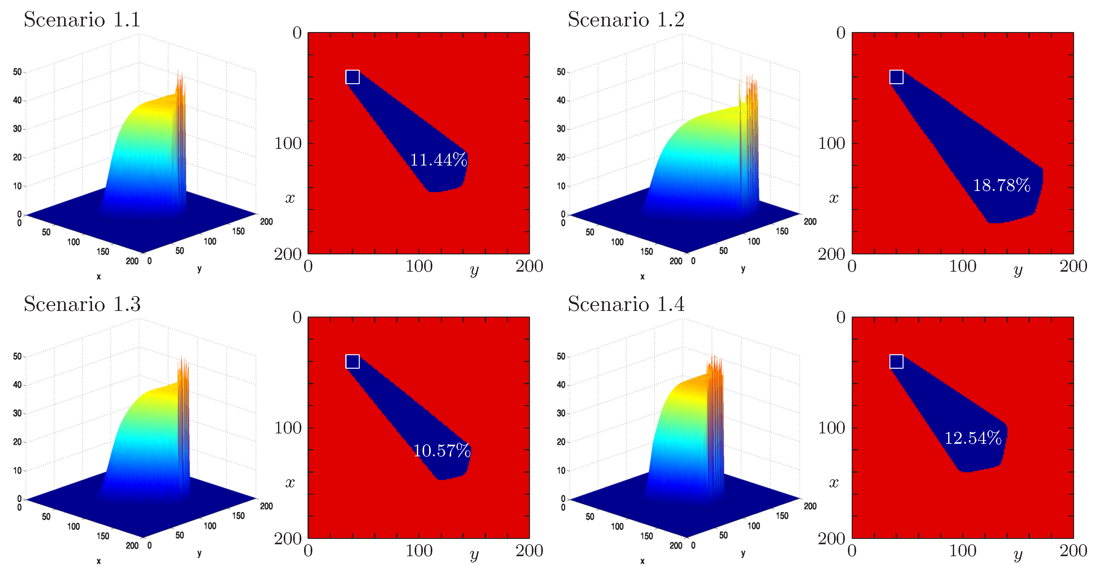
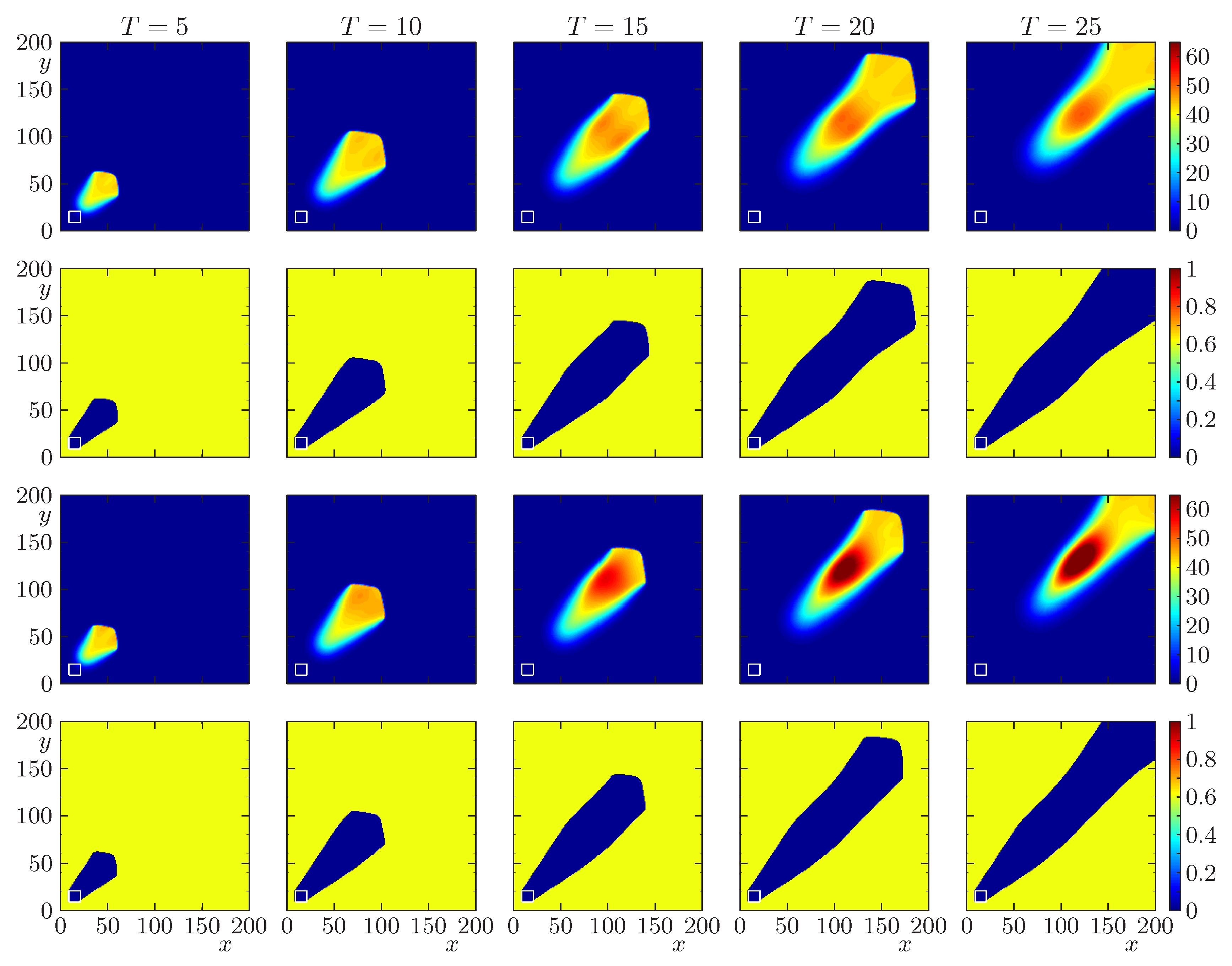
4.2. Scenarios 1.1 to 1.4: Numerical Experiments with Various Diffusion Coefficients

In this group of scenarios, we explore the influence of the dynamics of the combustion model. To this end we fix the initial distribution of temperature and that of fuel, and assume that the terrain is flat and homogeneous, but vary the diffusion function $K\left(u\right)$ to illustrate the effect of different model assumptions. We assume that the initial distribution of fuel is constant, as well as that the topography is flat. Specifically, the initial datum for temperature corresponds to an initial focus on a small square subdomain, i.e., we set

$$\begin{array}{c}\hfill u_0=\left\{\begin{array}{cc}21\hfill & \mathrm{for}(x,y)\in {[34,46]}^2,\hfill \\ 0\hfill & \mathrm{elsewhere}\hfill \end{array}\right.\end{array}$$

along with

$$\begin{array}{c}\hfill v_0(x,y)=0.9\mathrm{for}\mathrm{all}(x,y)\in \mathsf{\Omega }.\end{array}$$

With these initial data we simulate a base case and three variants of it. The base case, Scenario 1.1, is based on using the same remaining parameters and model functions as in [1], namely $K\left(u\right)$ defined by (5) with $\kappa =0.1$ and $\epsilon =0.035$, $f(u,v,\mathit{x})$ given by (6) with $c\left(u\right)$ defined through (7) with $u_{\mathrm{pc}}=20$ and $\alpha \equiv {10}^{-3}$, and $g(u,v)$ given by (8) with $q_{\mathrm{react}}=1$.

We are interested in comparing results with those obtained for alternative definitions of the diffusion coefficient $K\left(u\right)$. To this end, we repeat the simulation in Scenario 1.2 with the same parameters with the exception that $\kappa$ is five times larger, i.e., $\kappa =0.5$. Next, to motivate two alternative choices of the function $u\mapsto K\left(u\right)$, we recall first that the maximum temperature $u_{max}$ can be estimated from the ODE version of (1), (5)–(8), that is (10).

The result is that when we solve (10) for $t>0$ starting from $u\left(0\right)$ and $v\left(0\right)$, then $u\left(t\right)\le u_{max}:=(q_{\mathrm{react}}/\epsilon )v\left(0\right)+u\left(0\right)$. If we assume that in our case the relevant values are $v\left(0\right)=1$ and $u\left(0\right)=40$, then $u_{max}=1/0.035+40\approx 68.57=:u_{max}^{*}$. Thus, $K\left(u\right)$ assumes values between $K\left(0\right)=1.1$ and $K\left(u_{max}^{*}\right)=4.9304$. If we wish to compare results with those obtained for a constant diffusivity (as stipulated in [10]) $D\Delta u$ instead of $\nabla ·\left(K\right(u)\nabla u)$, then a reasonable value of the diffusion coefficient D for comparison should be

$$\begin{array}{c}\hfill D=\frac{1}{u_{max}^{*}}{\int }_0^{u_{{max}^{*}}}K\left(s\right)\mathrm{d}s=1+\frac{\kappa }{4\epsilon u_{max}^{*}}\left({(1+\epsilon u_{max}^{*})}^4-1\right)\approx 2.3816.\end{array}$$

Finally, we introduce the possibility of a degenerating diffusion coefficient, that is we allow that $K\left(u\right)=0$ for isolated values of u or even a u-interval of positive length. For instance, we may assume that the mechanisms of heat transfer are active only wherever u exceeds a critical value $u_{\mathrm{crit}}$. Applying this idea to the diffusion function $K\left(u\right)$ of Scenario 1.1, that is (5), we obtain

$$\begin{array}{c}\hfill K\left(u\right)=\left\{\begin{array}{cc}\kappa {(1+\epsilon u)}^3+1\hfill & \mathrm{for}u>u_{\mathrm{crit}},\hfill \\ 0\hfill & \mathrm{for}u\le u_{\mathrm{crit}}.\hfill \end{array}\right.\end{array}$$

(14)

For Scenario 1.4, we utilize (14) with $u_{\mathrm{crit}}=u_{\mathrm{pc}}=20$.

Figure 1 shows a plot of the diffusion functions for Scenarios 1.1 to 1.4, and Figure 2 displays the corresponding numerical results. Roughly speaking, Scenario 1.2 predicts a wildfire that has consumed a larger portion of fuel, and has travelled a larger distance, than that of Scenario 1.1. Far from the reaction front the maximum temperature in the combustion zone is slightly smaller. With a constant diffusion coefficient (Scenario 1.3) we obtain a less wide shape of the burnt area (in comparison with Scenario 1.1), and a smaller value of the burnt portion of fuel. Finally, as is to be expected with a strongly degenerating diffusion coefficient, the lateral flanks of the temperature surface of Scenario 1.4 are steeper than for all other scenarios.

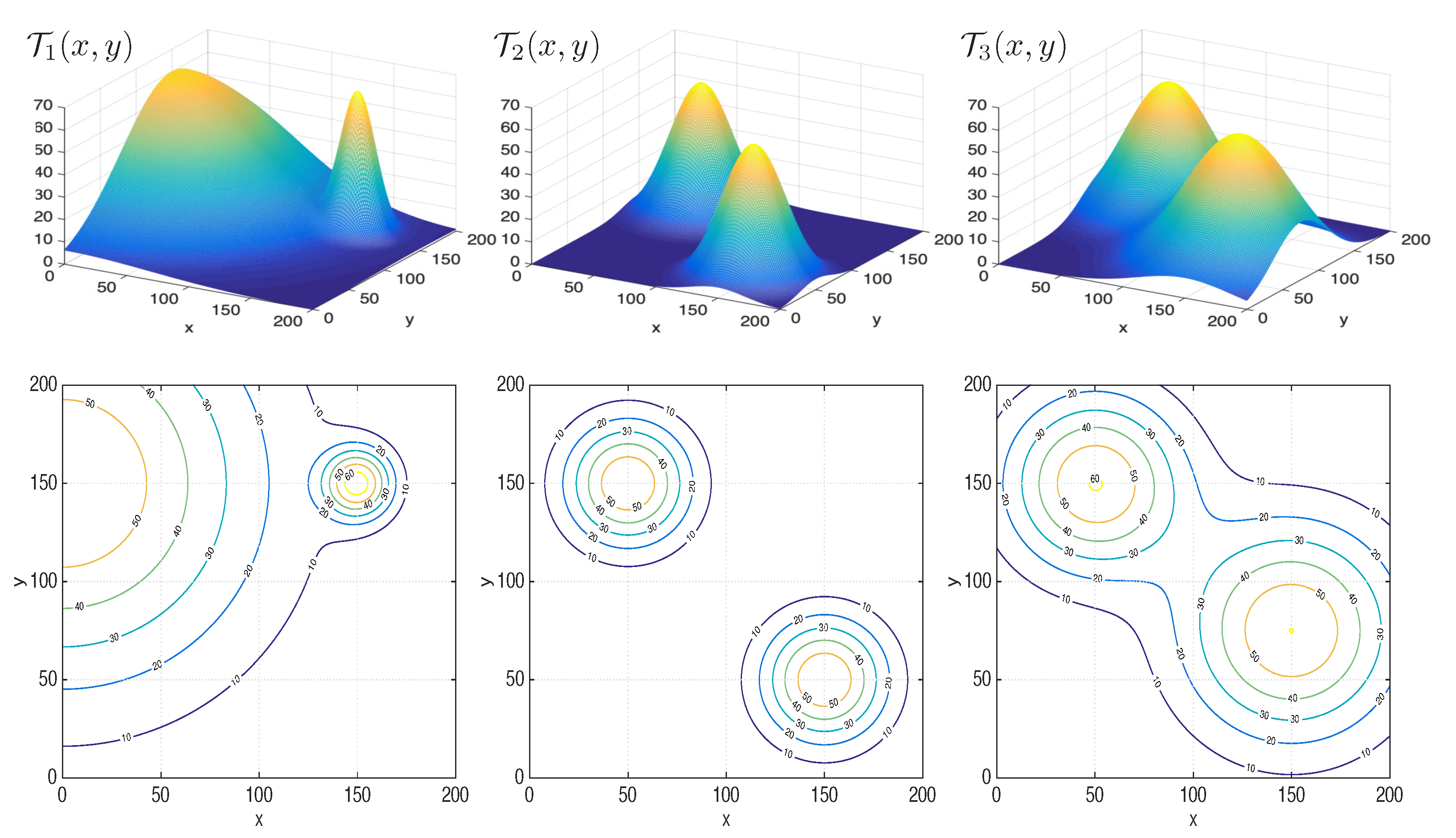
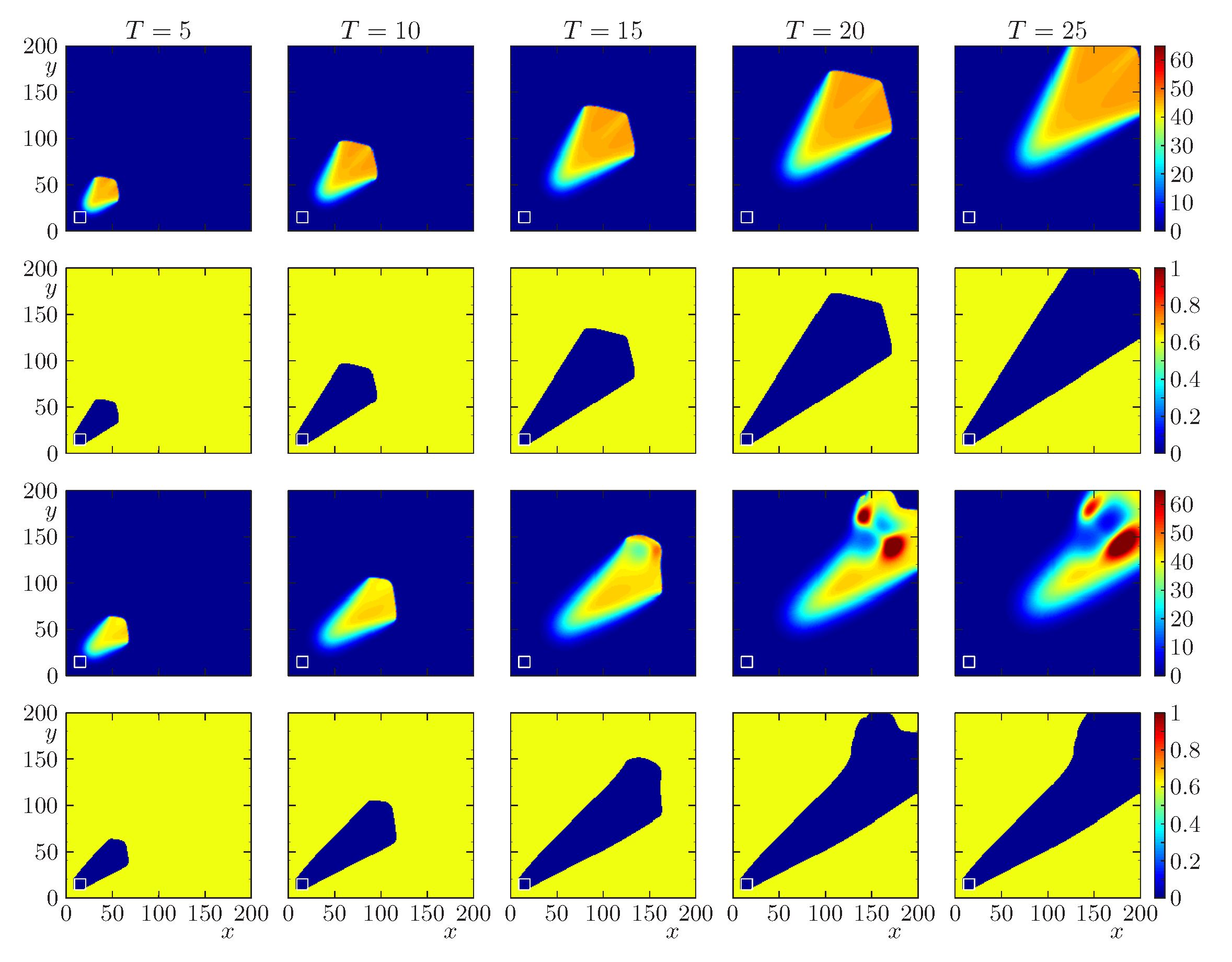
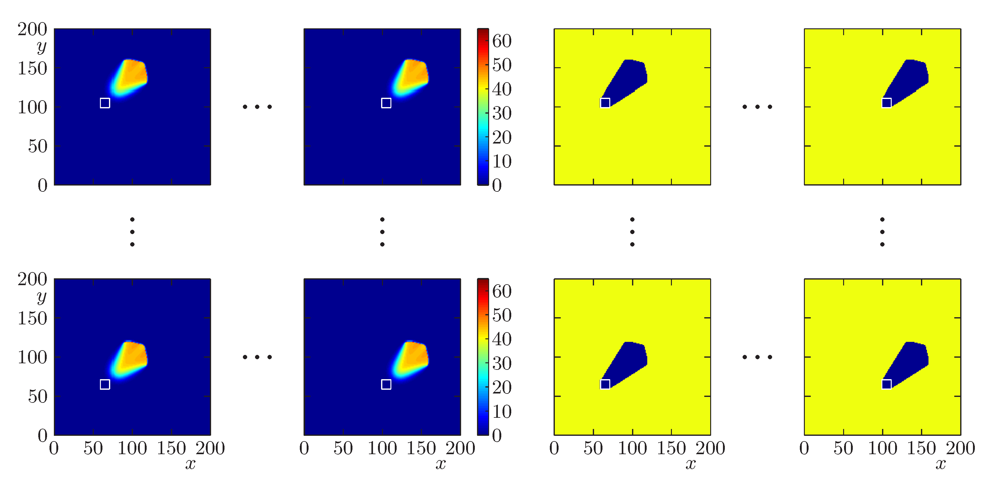
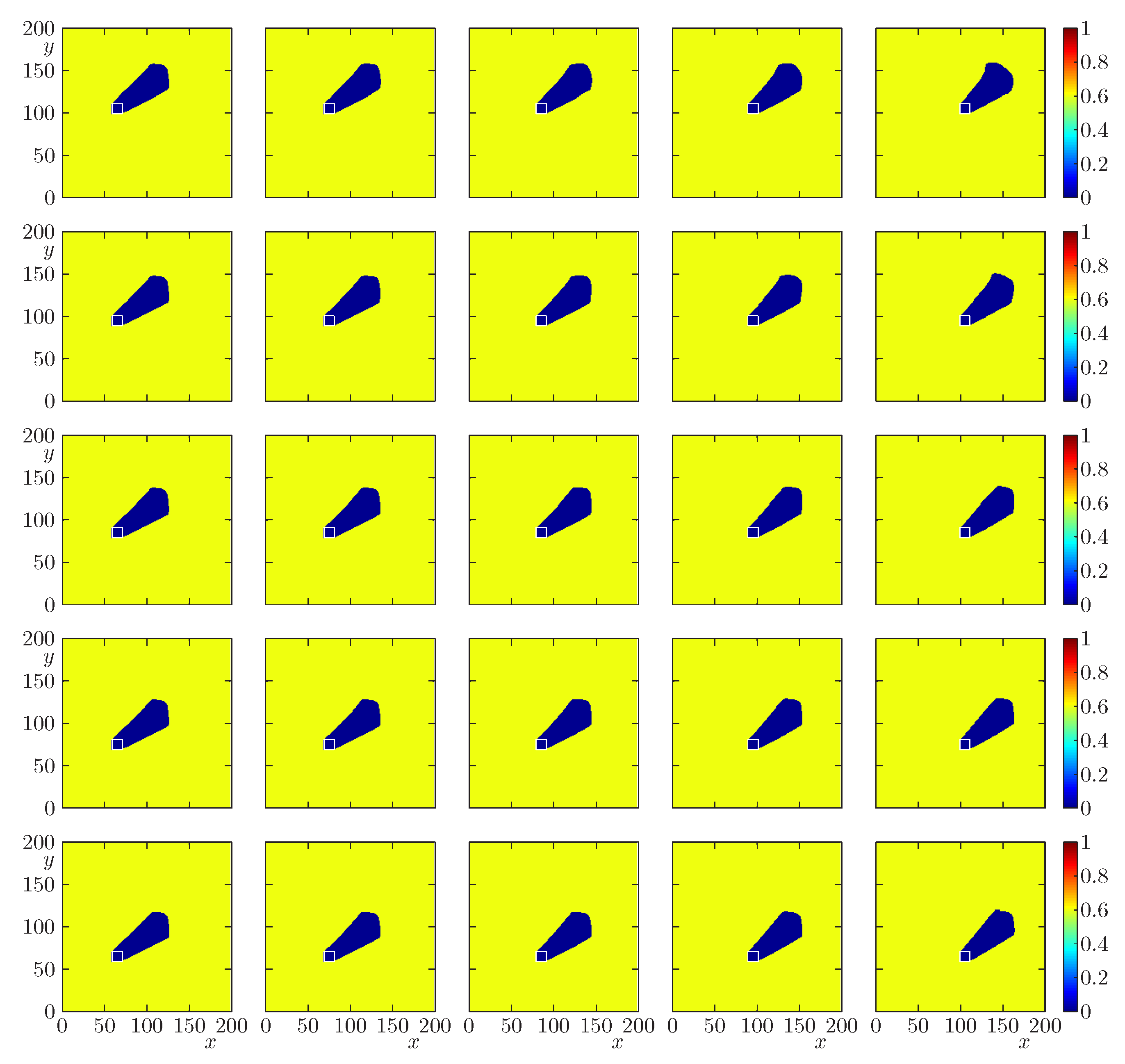
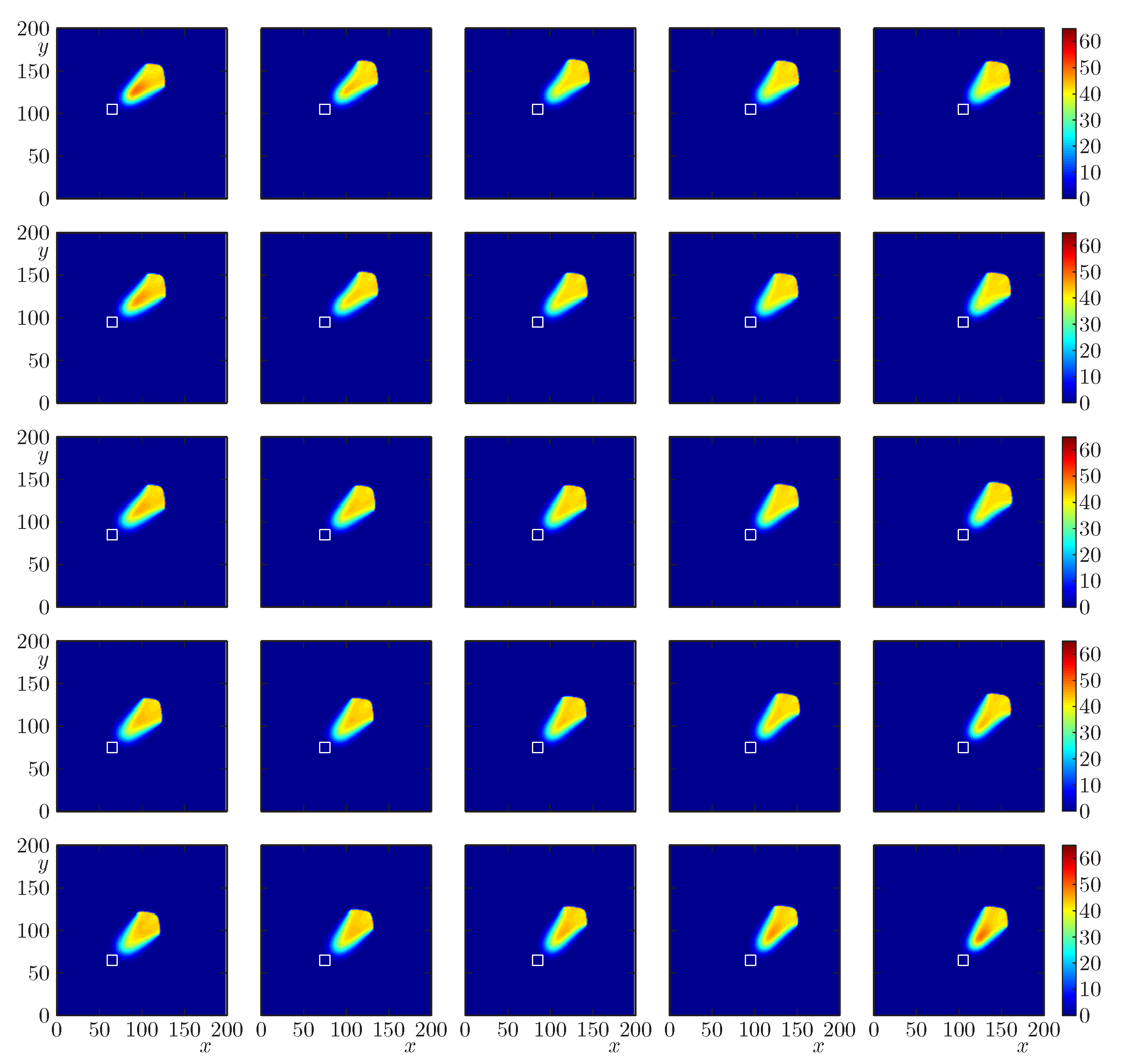
4.3. Scenarios 2.0 to 2.4: Effect of the Variability of Topography

In Scenario 2.0 we provide a comparison with a reference solution to show the numerical convergence of S-LIMEX scheme and in Scenarios 2.1 to 2.4 we study the net effect of terrain topography on the dynamics of wildfire propagation. To this end, we fix the diffusion function $K\left(u\right)$ as given by (5), and choose all other parameters as in Scenario 1.1 as well with the exception of $\epsilon =0.02$, with constant vector ${\mathit{w}}_0=(2.5,2.5)$ of velocity of the wind which blows in the north–east direction (that is, in the direction of increasing x- and y-coordinates). However, we assume various cases for the topography function $\mathcal{T}\left(\mathit{x}\right)=\mathcal{T}(x,y)$. To this end, and following [10], we define a shape function

$$\begin{array}{c}\hfill s(x,y;\gamma ):=exp\left(-(x^2+y^2)/\gamma \right)\mathrm{with}\mathrm{a}\mathrm{parameter}\gamma >0\end{array}$$

that describes a peak of height 1, centered at the origin. We assume that there are two peaks in the domain of variable height, as expressed by

$$\begin{array}{c}\hfill \mathcal{T}(x,y)=h_{1}s(x-x_1,y-y_1,{\gamma }_1)+h_{2}s(x-x_2,y-y_2,{\gamma }_2).\end{array}$$

(15)

For Scenario 2.0 we chose the parameters $(h_1,h_2,x_1,x_2,y_1,y_2,{\gamma }_1,{\gamma }_2)=(60,60,55,25,25,55,$$400,60)$ and three alternative choices of these parameters, in Scenarios 2.1 to 2.4, respectively, which are specified in the caption of Figure 3 that illustrates the variants of topography functions.

In

Table 1. Scenario 2.0: Approximate $L^1$ errors $e_M\left(u\right)$ and $e_M\left(v\right)$ for Strang LIMEX method with $\Delta x=80/M$. Reference solution computed with $M=640$.

$\mathit{T}=0.2$			$\mathit{T}=0.3$		$\mathit{T}=0.4$
$M$	$e_M\left(u\right)$	$e_M\left(v\right)$	$e_M\left(u\right)$	$e_M\left(v\right)$	$e_M\left(u\right)$	$e_M\left(v\right)$
40	2.2	3.7 $\times {10}^{-2}$	3.2	4.5$\times {10}^{-2}$	4.9	6.4$\times {10}^{-2}$
80	1.2	1.6 $\times {10}^{-2}$	2.0	2.3 $\times {10}^{-2}$	3.3	3.7$\times {10}^{-2}$
160	0.7	1.0 $\times {10}^{-2}$	1.2	1.5 $\times {10}^{-2}$	2.0	2.4$\times {10}^{-2}$
320	0.4	5.7 $\times {10}^{-3}$	0.6	8.9 $\times {10}^{-3}$	1.1	1.4$\times {10}^{-2}$

we compute the approximate $L^1$-errors $e_M\left(u\right)$ and $e_M\left(v\right)$ at three simulated time $T=0.2$, $T=0.3$ and $T=0.4$ with different discretizations by using $M=40$, 80, 160 and 320, with respect to reference solution computed with S-LIMEX scheme with $M=640$. We observe that the approximate $L^1$-errors decrease as the grid is refined, which can be also observed in Figure 4 where we display the numerical approximations for $M=160$ and $M=640$ at simulated times $T=0.2$ and $T=0.4$. We observe that the approximation obtained with $M=160$ is a already a good approximation of the reference solution.

For Scenarios 2.1 to 2.4, the initial conditions of temperature and fuel are

$$\begin{array}{c}\hfill u_0(x,y)=21{\chi }_{{\left[9,21\right]}^2}(x,y),v_0(x,y)=0.6{\chi }_{\mathsf{\Omega }}(x,y).\end{array}$$

We display the numerical approximation obtained at simulated times $T=5$, 10, 15, 20, and 25. We display the evolutions of the temperature and fuel over a flat domain and topography ${\mathcal{T}}_1$ in Figure 5, and show the analogous results for topographies ${\mathcal{T}}_2$ and ${\mathcal{T}}_3$ in Figure 6. In the cases ${\mathcal{T}}_1,{\mathcal{T}}_2$ and ${\mathcal{T}}_3$ the topography acts as repulsion, which moves away the propagation fires (Figure 5 third and fourth row) or centers the propagation on the diagonal of the domain (Figure 6 first and second row) respectively.

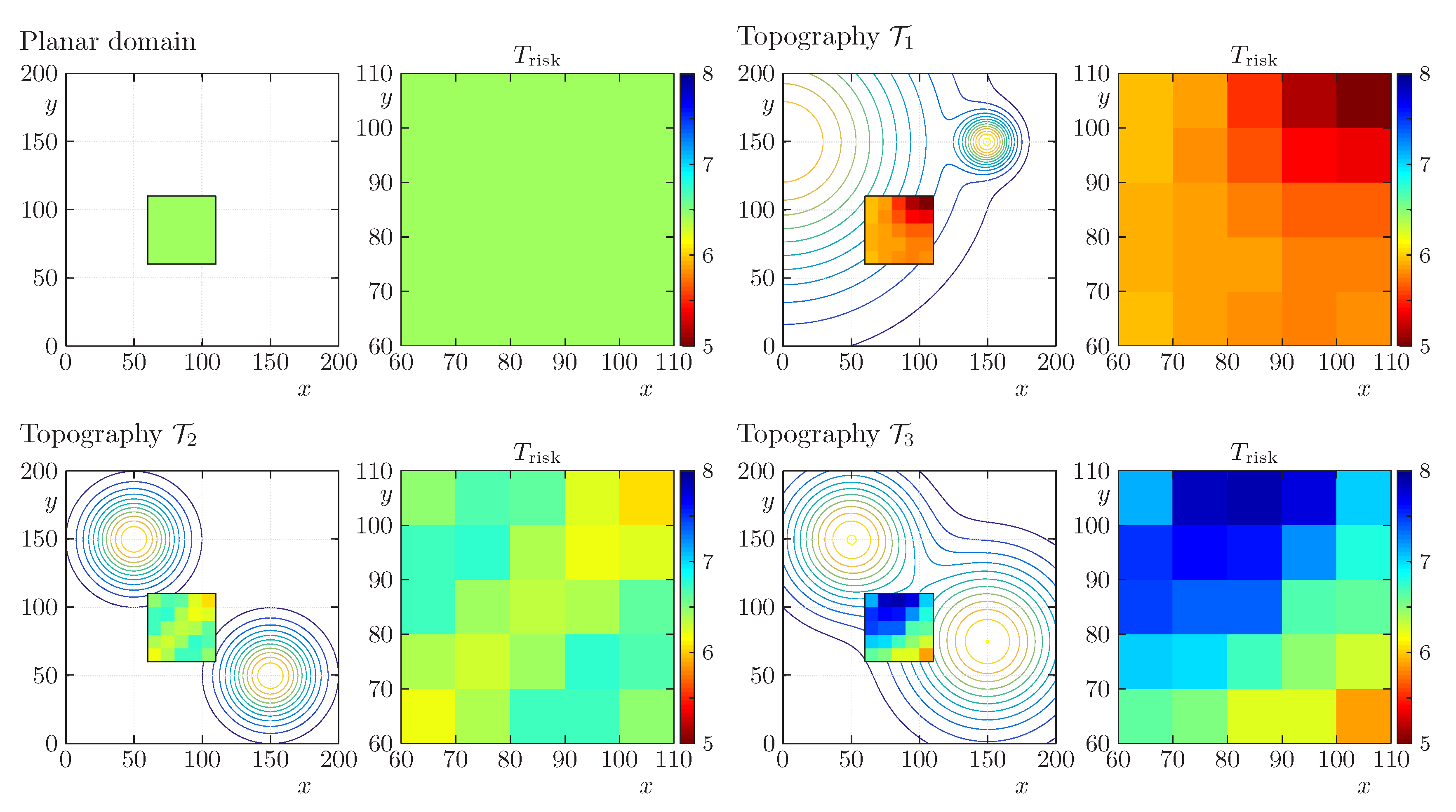
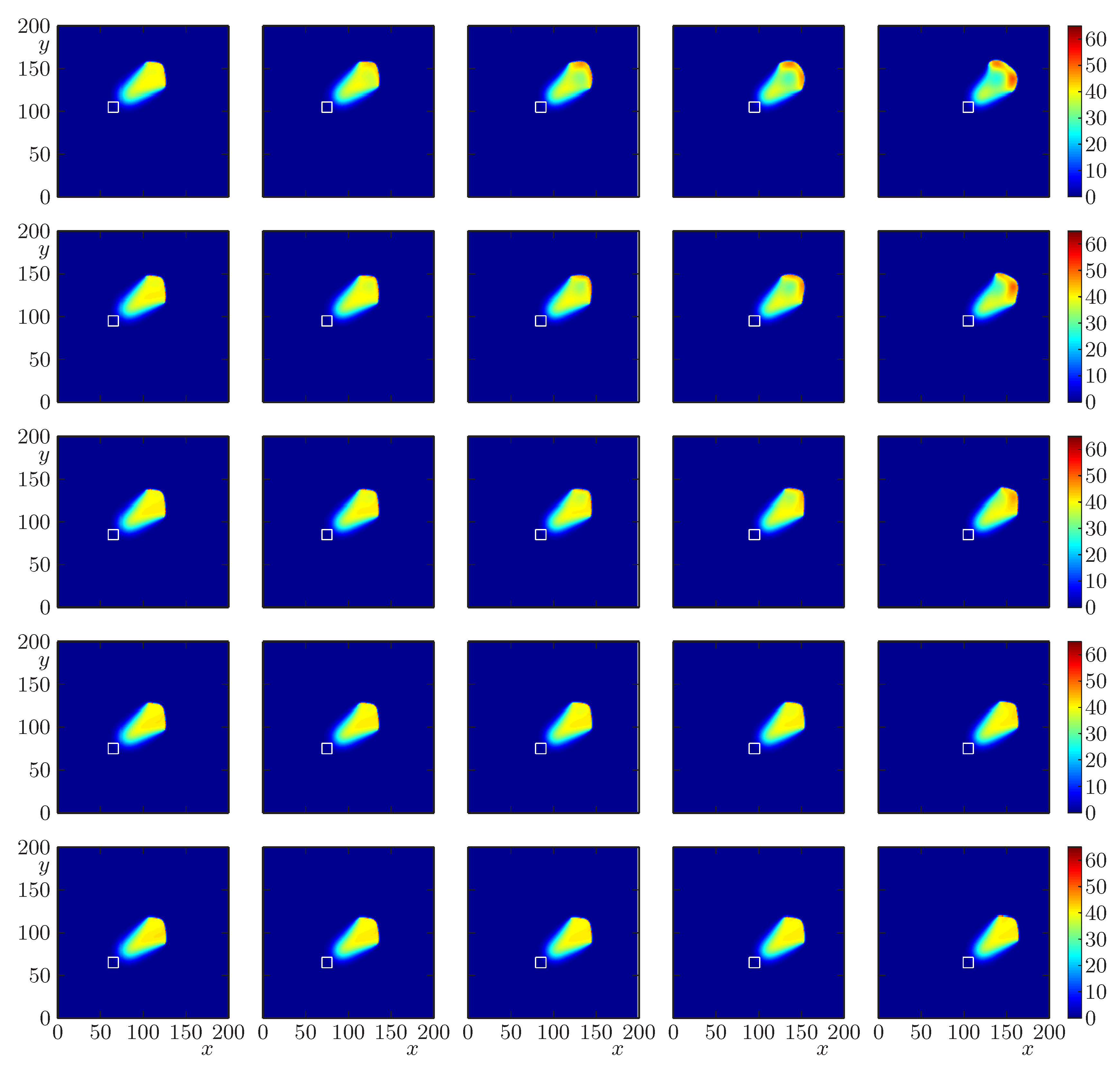
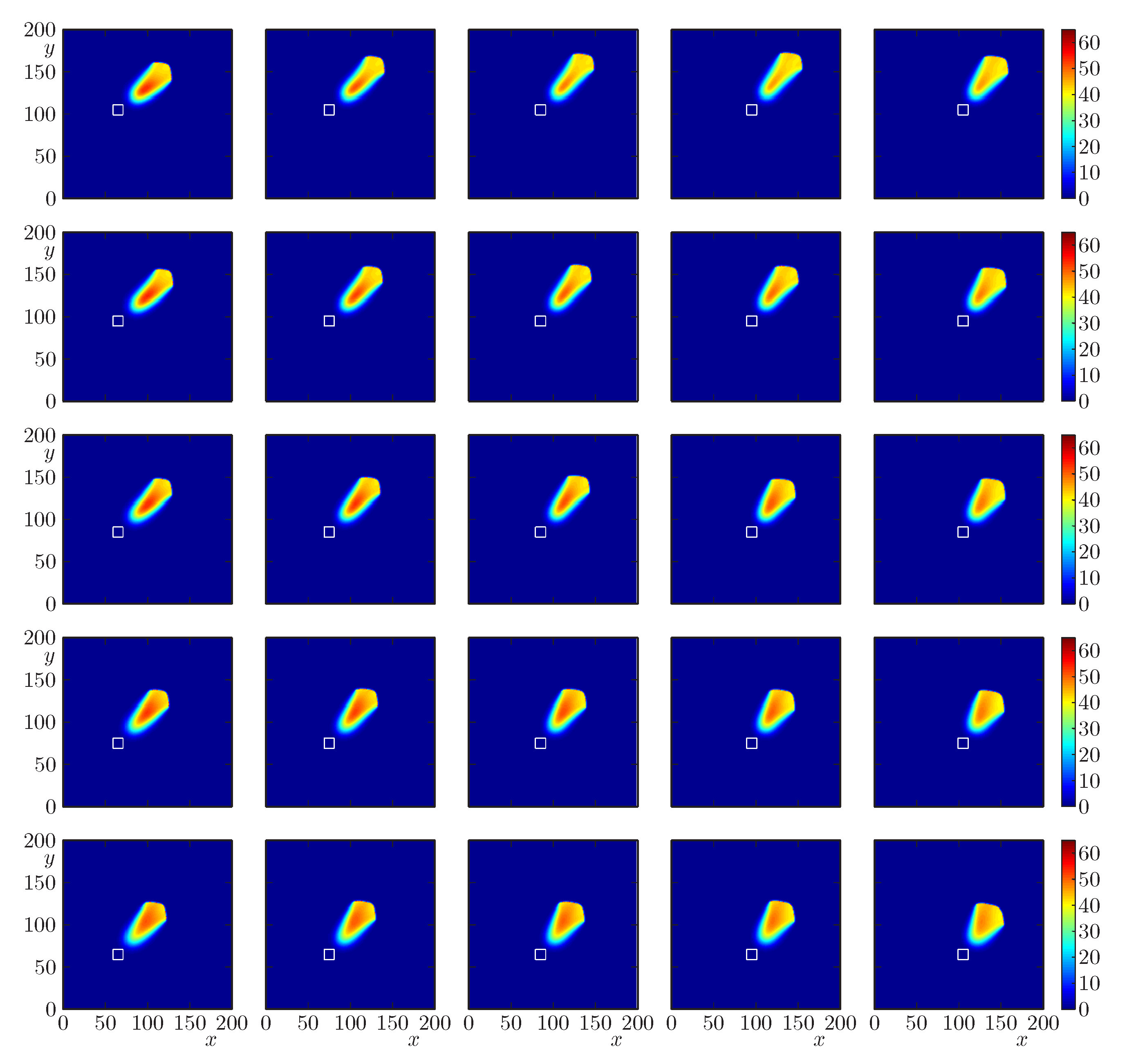
4.4. Scenarios 3.1 to 3.4: Risk Maps

An analysis that is interesting when studying the effects of topography on the source of fire in a forest fire is the elaboration of the so-called risk maps, which we present in this section. To do this we consider four cases here, the first corresponds to the absence of the variable $\mathcal{T}$ where we are in the presence of a perfectly flat terrain and three other cases which correspond to each of the topographies ${\mathcal{T}}_1$, ${\mathcal{T}}_2$ and ${\mathcal{T}}_3$ of the previous section. Each of the risk maps constructed corresponds to square initial ignitions of length 12 placed on

$$\begin{array}{c}\hfill D_{ij}:=\left\{(x,y)\in \mathsf{\Omega }\mid |x-(55+10i\left)\right|\le 6,|y-(55+10j\left)\right|\le 6\right\},i,j=1,\cdots ,5,\end{array}$$

(16)

which yields a total number of 25 initial foci.

The risk maps indicate the different values obtained for the time $T_{\mathrm{risk}}$ when the focus of the fire takes to consume 5% of the total fuel available in the domain, so a short time corresponds to a high risk and a long time corresponds to a low risk. In each of the four cases (of a flat domain and a domain with one of the topographies ${\mathcal{T}}_1$, ${\mathcal{T}}_2$ and ${\mathcal{T}}_3$) the ignitions are located in the south-west of the original domain. Specifically, to assign a value of $T_{\mathrm{risk}}$ to each of the patches of size $10\times 10$

$$\begin{array}{c}\hfill D_{ij}^0:=\left\{(x,y)\in \mathsf{\Omega }\mid |x-(55+10i\left)\right|\le 5,|y-(55+10j\left)\right|\le 5\right\},i,j=1,\cdots ,5,\end{array}$$

we simulate the wildfire model starting from the initial condition

$$u_0(x,y)=21{\chi }_{D_{ij}}(x,y),v_0(x,y)=0.6,$$

where $D_{ij}$ is specified (16) and the velocity is given by $\mathit{w}={\mathit{w}}_0$ in the flat case, $\mathit{w}={\mathit{w}}_0+\nabla {\mathcal{T}}_i$, $i=1,2,3$ for the non-flat topographies, and ${\mathit{w}}_0=(2.5,2.5)$. The result is in each case a risk map for the domain $[60,110]\times [60,110]$, with a (fairly coarse) resolution of 25 patches of size $10\times 10$.

In the case of flat terrain the propagation of fire and burnt fuel always have the same spatio-temporal evolution but shifted according to the location of the initial focus (Figure 7) and 5% of the total available fuel is consumed, the time in the 25 foci is identical and it corresponds to $T_{\mathrm{risk}}=6.45$ and the risk map obtained which can be seen in the top left plots of Figure 8 corresponds to a high-risk scenario (but the risk is the same for each $10\times 10$ patch).

For the topography ${\mathcal{T}}_1$, all the values obtained for the time in which 5% of fuel consumed is reached are in less time than $T_{\mathrm{risk}}=6.45$ being the minimum value $T_{\mathrm{risk}}=4.92$ that is reached on ${[100,110]}^2$ and the maximum value $T_{\mathrm{risk}}=5.98$ that is reached on $[60,70]\times [100,110]$. The evolution of temperature and fuel can be seen in Figure 9 and Figure 10 and the risk map obtained, which is displayed on the top right of Figure 8, corresponds to a slightly higher risk to the case of flat a terrain.

In the case of topography ${\mathcal{T}}_2$, the minimum value $T_{\mathrm{risk}}=6.04$ is reached on $[60,70]\times [100,110]$ and the maximum value $T_{\mathrm{risk}}=6.77$ that is reached on ${[80,90]}^2$. The evolution of temperature and fuel can be seen in Figure 11 and Figure 12 and the risk map obtained which can be seen in the bottom left part of Figure 8 corresponds to similar risk to the flat a terrain.

For topography ${\mathcal{T}}_3$, the majority of values are higher than $T_{\mathrm{risk}}=6.45$ being the minimum value $T_{\mathrm{risk}}=5.85$ that is attained on $[90,100]\times [60,70]$ and the maximum value $T_{\mathrm{risk}}=7.90$ that is reached on $[80,90]\times [100,110]$. The evolution of temperature and fuel can be seen in Figure 13 and Figure 14 and the risk map obtained which can be seen in the bottom right part of Figure 8 corresponds to a low-risk scenario.

5. Conclusions

In the present work we analyzed the wildland fire model in [5] to simulate the propagation of a wildfire in various spatially heterogeneous environments. In particular, we focus on variable, nonlinear diffusion functions to explore the dynamics of the combustion model and a variable topography function to analyze the effects of the spatial heterogeneity. This model was solved numerically in an efficient way by the numerical method proposed in [1].

Several diffusion functions are explored (Scenarios 1.1 to 1.4) to arrive at the conclusion that these functions are strongly related to the shape of the burnt area. The main result is that increasing diffusivity (with respect to a given base case) significantly enlarges the portion of fuel burnt within a given time while choosing an equivalent constant diffusivity or a degenerate one produces comparable results for that quantity. Considering three different topographies, we were able to show how the terrain affects the spread of the forest fire, acting as an element that manages to increase fuel consumption (Scenarios 2.2 and 2.4) but also as an element that manages to vary the direction of fire spread acting as a repulsion (Scenario 2.3) which pushes it toward areas far from its initial trajectory (Scenario 2.2). On the other hand, due to the shapes of the landscape, in two of these cases it is possible to capture how the elevation of the ground manages to accelerate the spread of fire (see Appendix B in [44]).

Considering that a determining factor in the spread of fire is the value of the slope associated with the terrain, in the sense that the higher the slope, said spread occurs more quickly, it is essential to obtain the times in which a certain constant portion of the fuel has been consumed through the risk maps (see Figure 8). Finally, the possibility to solve the base model efficiently may be used as a tool to elaborate wildfire risk maps.

The verification and calibration of the model taking into account data from real wildfires in four of the authors’ geographic environment (Chile) is still an open issue, while scenarios related to other geographic regions are successfully simulated in [4] (Germany) and [8,9] (varios regions of Spain). Clearly, realistic scenarios can be considered if geographical information and meteorological data are integrated, which can be achieved through a Geographical Information System (GIS). We refer to [8] for details and mention that we are currently making the effort to access similar information for Chile. On the other hand, and as we mentioned in [1], another omission is the neglect of moisture and pyrolysis effects that can be handled via a multivalued enthalpy function [5,6].

References

1. Bürger, R.; Gavilán, E.; Inzunza, D.; Mulet, P.; Villada, L.M. Implicit–explicit methods for a convection-diffusion-reaction model of the propagation of forest fires. Mathematics 2020, 8, 1034. [Google Scholar] [CrossRef]
2. Asensio, M.I.; Ferragut, L. On a wildland fire model with radiation. Int. J. Numer. Methods Eng. 2002, 54, 137–157. [Google Scholar] [CrossRef]
3. Pastor, E.; Zárate, L.; Planas, E.; Arnaldos, J. Mathematical models and calculation systems for the study of wildland fire behaviour. Prog. Energy Combust. Sci. 2003, 29, 139–153. [Google Scholar] [CrossRef]
4. Eberle, S.; Freeden, W.; Matthes, U. Forest fire spreading. In Handbook of Geomathematics, 2nd ed.; Freeden, W., Nashed, M.Z., Sonar, T., Eds.; Springer: Berlin, Germany, 2015; pp. 1349–1385. [Google Scholar]
5. Ferragut, L.; Asensio, M.I.; Monedero, S. Modelling radiation and moisture content in fire spread. Commun. Numer. Methods Eng. 2007, 23, 819–833. [Google Scholar] [CrossRef]
6. Ferragut, L.; Asensio, M.I.; Monedero, S. A numerical method for solving convection-reaction-diffusion multivalued equations in fire spread modelling. Adv. Eng. Softw. 2007, 38, 366–371. [Google Scholar] [CrossRef]
7. Asensio, M.I.; Ferragut, L.; Simon, J. A convection model for fire spread simulation. Appl. Math. Lett. 2005, 18, 673–677. [Google Scholar] [CrossRef]
8. Prieto, D.; Asensio, M.I.; Ferragut, L.; Cascón, J.M.; Morillo, A. A GIS-based fire spread simulator integrating a simplified physical wildland fire model and a wind field model. Int. J. Geogr. Inf. Sci. 2017, 31, 2142–2163. [Google Scholar] [CrossRef]
9. Ferragut, L.; Asensio, M.I.; Cascón, J.M.; Prieto, D. A simplified wildland fire model applied to a real case. In Advances in Differential Equations and Applications; Casas, F., Martínez, V., Eds.; SEMA Springer Series 4; Springer International Publishing: Cham, Switzerland, 2014; pp. 155–167. [Google Scholar]
10. San Martín, D.; Torres, C.E. Ngen-Kütral: Toward an open source framework for Chilean wildfire spreading. In Proceedings of the 37th International Conference of the Chilean Computer Science Society (SCCC), Santiago, Chile, 5–9 November 2018; pp. 1–8. [Google Scholar]
11. San Martín, D.; Torres, C.E. Exploring a spectral numerical algorithm for solving a wildfire mathematical model. In Proceedings of the 38th International Conference of the Chilean Computer Science Society (SCCC), Concepción, Chile, 4–9 November 2019; pp. 1–7. [Google Scholar]
12. Barovik, D.; Taranchuk, V. Mathematical modelling of running crown forest fires. Math. Model. Anal. 2010, 15, 161–174. [Google Scholar] [CrossRef] [Green Version]
13. Taranchuk, V.; Barovik, D. Numerical modeling of surface forest fire spread in nonuniform woodland. In Computer Algebra Systems in Teaching and Research Vol. VIII; Prokopenya, A.N., Gil-Świderska, A., Siłuszyk, M., Eds.; Siedlce University of Natural Sciences and Humanities, Institute of Mathematics and Physics: Siedlce, Poland, 2019; pp. 159–168. [Google Scholar]
14. Bebernes, J.; Eberly, D. Mathematical Problems from Combustion Theory; Springer: New York, NY, USA, 1989. [Google Scholar]
15. Glassman, I.; Yetter, R.A.; Glumac, N.G. Combustion, 5th ed.; Academic Press: Boston, MA, USA, 2015. [Google Scholar]
16. Séro-Guillaume, O.; Margerit, J. Modelling forest fires. Part I: A complete set of equations derived by extended irreversible thermodynamics. Int. J. Heat Mass Transf. 2002, 45, 1705–1722. [Google Scholar] [CrossRef]
17. Margerit, J.; Séro-Guillaume, O. Modelling forest fires. Part II: Reduction to two-dimensional models and simulation of propagation. Int. J. Heat Mass Transf. 2002, 45, 1723–1737. [Google Scholar] [CrossRef]
18. Linn, R.R.; Canfield, J.M.; Cunningham, P.; Edminster, C.; Dupuy, J.-L.; Pimont, F. Using periodic line fires to gain a new perspective on multi-dimensional aspects of forward fire spread. Agric. For. Meteorol. 2012, 157, 60–76. [Google Scholar] [CrossRef]
19. Moinuddin, K.A.M.; Sutherland, D. Modeling of tree fires and fires transitioning from the forest floor to the canopy with a physics-based model. Math. Comput. Simul. 2020, 175, 81–95. [Google Scholar] [CrossRef]
20. Hundsdorfer, W.; Verwer, J.G. Numerical Solution of Time-Dependent Advection-Diffusion-Reaction Equations; Springer: Berlin, Germany, 2003. [Google Scholar]
21. Butcher, J.C. Numerical Methods for Ordinary Differential Equations, 2nd ed.; Wiley: Chichester, UK, 2008. [Google Scholar]
22. Hairer, E.; Nørsett, S.P.; Wanner, G. Solving Ordinary Differential Equations. I. Non-Stiff Problems; Springer Series in Computational Mathematics; Springer: Berlin, Germany, 1993; Volume 8. [Google Scholar]
23. Ascher, U.; Ruuth, S.; Spiteri, J. Implicit-explicit Runge-Kutta methods for time dependent partial differential equations. Appl. Numer. Math. 1997, 25, 151–167. [Google Scholar] [CrossRef]
24. Pareschi, L.; Russo, G. Implicit-Explicit Runge-Kutta schemes and applications to hyperbolic systems with relaxation. J. Sci. Comput. 2005, 25, 129–155. [Google Scholar]
25. Boscarino, S.; Bürger, R.; Mulet, P.; Russo, G.; Villada, L.M. Linearly implicit IMEX Runge-Kutta methods for a class of degenerate convection-diffusion problems. SIAM J. Sci. Comput. 2015, 37, B305–B331. [Google Scholar] [CrossRef]
26. Boscarino, S.; Bürger, R.; Mulet, P.; Russo, G.; Villada, L.M. On linearly implicit IMEX Runge-Kutta Methods for degenerate convection-diffusion problems modelling polydisperse sedimentation. Bull. Braz. Math. Soc. (New Ser.) 2016, 47, 171–185. [Google Scholar] [CrossRef]
27. Boscarino, S.; Filbet, F.; Russo, G. High order semi-implicit schemes for time dependent partial differential equations. J. Sci. Comput. 2016, 68, 975–1001. [Google Scholar] [CrossRef] [Green Version]
28. Boscarino, S.; LeFloch, P.G.; Russo, G. High order asymptotic-preserving methods for fully nonlinear relaxation problems. SIAM J. Sci. Comput. 2014, 36, A377–A395. [Google Scholar] [CrossRef]
29. Donat, R.; Guerrero, F.; Mulet, P. Implicit-explicit methods for models for vertical equilibrium multiphase flow. Comput. Math. Appl. 2014, 68, 363–383. [Google Scholar] [CrossRef]
30. Bürger, R.; Chowell, G.; Gavilán, E.; Mulet, P.; Villada, L.M. Numerical solution of a spatio-temporal gender-structured model for hantavirus infection in rodents. Math. Biosci. Eng. 2018, 15, 95–123. [Google Scholar] [CrossRef] [Green Version]
31. Bürger, R.; Chowell, G.; Gavilán, E.; Mulet, P.; Villada, L.M. Numerical solution of a spatio-temporal predator-prey model with infected prey. Math. Biosci. Eng. 2019, 16, 438–473. [Google Scholar] [CrossRef]
32. Bürger, R.; Goatin, P.; Inzunza, D.; Villada, L.M. A non-local pedestrian flow model accounting for anisotropic interactions and domain boundaries. Math. Biosci. Eng. 2020, 17, 5883–5906. [Google Scholar]
33. Bürger, R.; Inzunza, D.; Mulet, P.; Villada, L.M. Implicit-explicit schemes for nonlinear nonlocal equations with a gradient flow structure in one space dimension. Numer. Methods Partial Differ. Equ. 2019, 35, 1008–1034. [Google Scholar] [CrossRef]
34. Bürger, R.; Inzunza, D.; Mulet, P.; Villada, L.M. Implicit-explicit methods for a class of nonlinear nonlocal gradient flow equations modelling collective behaviour. Appl. Numer. Math. 2019, 144, 234–252. [Google Scholar] [CrossRef]
35. Bürger, R.; Mulet, P.; Villada, L.M. Regularized nonlinear solvers for IMEX methods applied to diffusively corrected multi-species kinematic flow models. SIAM J. Sci. Comput. 2013, 35, B751–B777. [Google Scholar] [CrossRef]
36. Abgrall, R.; Shu, C.-W. Handbook of Numerical Analysis for Hyperbolic Problems. Basic and Fundamental Issues; North-Holland: Amsterdam, The Netherlands, 2016. [Google Scholar]
37. Shu, C.-W. Essentially non-oscillatory and weighted essentially non-oscillatory schemes for hyperbolic conservation laws. In Advanced Numerical Approximation of Nonlinear Hyperbolic Equations; Quarteroni, A., Ed.; Lecture Notes in Mathematics; Springer: Berlin, Germany, 1998; Volume 1697, pp. 325–432. [Google Scholar]
38. Shu, C.-W. High order weighted essentially nonoscillatory schemes for convection dominated problems. SIAM Rev. 2009, 51, 82–126. [Google Scholar] [CrossRef] [Green Version]
39. LeVeque, R.J. Finite Volume Methods for Hyperbolic Problems; Cambridge University Press: Cambridge, UK, 2002. [Google Scholar]
40. Hesthaven, J.S. Numerical Methods for Conservation Laws; Society for Industrial and Applied Mathematics: Philadelphia, PA, USA, 2018. [Google Scholar]
41. Marin, M.; Vlase, S.; Paun, M. Considerations on double porosity structure for micropolar bodies. AIP Adv. 2015, 5, 037113. [Google Scholar] [CrossRef] [Green Version]
42. Holden, H.; Karlsen, K.H.; Lie, K.-A.; Risebro, N.H. Splitting Methods for Partial Differential Equations with Rough Solutions; European Mathematical Society: Zurich, Switzerland, 2010. [Google Scholar]
43. Strang, G. On the construction and comparison of difference schemes. SIAM J. Numer. Anal. 1968, 5, 506–517. [Google Scholar] [CrossRef]
44. Bennett, M.; Fitzgerald, S.A.; Parker, B.; Main, M.L.; Perleberg, A.; Schnepf, C.; Mahoney, R.L. Reduce the Risk of Fire on Your Forest Property; Oregon State University: Corvallis, OR, USA, 2010. [Google Scholar]
Figure 1. Scenarios 1.1 to 1.4: diffusion coefficients K ( u ) .
Mathematics 08 01674 g001
Figure 2. Scenarios 1.1 to 1.4: three-dimensional plots of simulated temperature and two-dimensional plots of simulated burnt fuel, at simulated time T = 12 . The red and blue parts correspond to areas with v 0 = 0.9 and v 0 = 0 , respectively. The small white square indicates the location of the initial fire focus. The percentages represent the portion of burnt fuel of the total fuel initially available in Ω .
Mathematics 08 01674 g002
Figure 3. Topographies for T ( x , y ) given by (15) with h 1 = h 2 = 60 and (left) x 1 = 0 , y 1 = 150 , γ 1 = 10 , 000 , x 2 = 150 , y 2 = 150 , γ 2 = 300 (topography T 1 for Scenario 2.2), (middle) x 1 = 150 , y 1 = 50 , γ 1 = 1000 , x 2 = 50 , y 2 = 150 , γ 2 = 1000 (topography T 2 for Scenario 2.3), (right) x 1 = 150 , y 1 = 75 , γ 1 = 3000 , x 2 = 50 , y 2 = 150 , γ 2 = 2000 (topography T 3 for Scenario 2.4), shown in each case as three-dimensional plots (top) and as contour maps (bottom).
Mathematics 08 01674 g003
Figure 4. Scenario 2.0: accuracy test. Numerical approximations at simulated time T = 0.2 and T = 0.4 obtained with the S-LIMEX scheme with Δ x = 80 / M and M = 160 and M = 640 (which correspond to the reference solution for computation of approximate errors in Table 1).
Mathematics 08 01674 g004
Figure 5. Scenarios 2.1 and 2.2: simulation of the propagation of a forest fire on a flat domain (first and second row) and on a domain with topography T 1 (third and fourth row), at indicated simulated times. Here and in Figure 6, the first and third row show temperature and the second and fourth row show fuel, and small white square indicates the location of the initial wildfire.
Mathematics 08 01674 g005
Figure 6. Scenarios 2.3 and 2.4: simulation of the propagation of a forest fire on domains with topographies T 2 (first and second row) and T 3 (third and fourth row).
Mathematics 08 01674 g006
Figure 7. Scenario 3.1: principle of construction of a risk map for a flat domain. Here and in Scenarios 3.2 to 3.4, the propagation of a wildfire is simulated starting from an array of 5 × 5 = 25 initial fire foci, marked by small white squares. For each initial position the simulation is stopped when 5 % of the initially available fuel is burnt. The corresponding times T risk are mapped in Figure 8. (For the present flat case, the shapes of the temperature and fuel distributions are the always the same in relation to the initial fire; instead of displaying 2 × 25 identical results, we only show the ‘corner’ cases of the 5 × 5 initial positions).
Mathematics 08 01674 g007
Figure 8. Scenarios 3.1 to 3.4: risk maps for the subdomain [ 60 , 110 ] × [ 60 , 110 ] under the assumption of a flat domain (Scenario 3.1, top left) and domains with topography T 1 , T 2 , and T 3 (Scenarios 3.2 to 3.4, top right, bottom left, and bottom right), visualizing for each patch of size 10 × 10 the final time T risk . A low value of T risk implies a high risk.
Mathematics 08 01674 g008
Figure 9. Scenario 3.2: simulation of temperature of a wildfire from 5 × 5 = 25 initial fire foci, marked by small white squares, on a domain with topography T 1 . Here and in Figure 10, Figure 11, Figure 12, Figure 13 and Figure 14, for each initial position where the simulation is stopped, and the numerical solutions for u and v are portrayed, when 5 % of the initially available fuel is burnt. The corresponding simulated time determines T risk for each initial position.
Mathematics 08 01674 g009
Figure 10. Scenario 3.2: simulation of fuel of a wildfire from 5 × 5 = 25 initial fire foci, marked by small white squares, on a domain with topography T 1 .
Mathematics 08 01674 g010
Figure 11. Scenario 3.3: simulation of temperature of a wildfire from 5 × 5 = 25 initial fire foci, marked by small white squares, on a domain with topography T 2 .
Mathematics 08 01674 g011
Figure 12. Scenario 3.3: simulation of fuel of a wildfire from 5 × 5 = 25 initial fire foci, marked by small white squares, on a domain with topography T 2 .
Mathematics 08 01674 g012
Figure 13. Scenario 3.4: simulation of temperature of a wildfire from 5 × 5 = 25 initial fire foci, marked by small white squares, on a domain with topography T 3 .
Mathematics 08 01674 g013
Figure 14. Scenario 3.4: simulation of fuel of a wildfire from 5 × 5 = 25 initial fire foci, marked by small white squares, on a domain with topography T 3 .
Mathematics 08 01674 g014