Article

Exact Solutions to the Maxmin Problem max‖Ax‖ Subject to ‖Bx‖≤1

1
Department of Mathematics, College of Engineering, University of Cadiz, 11510 Puerto Real, Spain
2
Department of Electronics, College of Engineering, University of Cadiz, 11510 Puerto Real, Spain
3
Department of Statistics and Operation Research, College of Engineering, University of Cadiz, 11510 Puerto Real, Spain
*
Author to whom correspondence should be addressed.
These authors contributed equally to this work.
Mathematics 2020, 8(1), 85; https://doi.org/10.3390/math8010085
Submission received: 15 October 2019 / Revised: 28 December 2019 / Accepted: 30 December 2019 / Published: 4 January 2020
(This article belongs to the Special Issue Numerical Methods)

Abstract

:
In this manuscript we provide an exact solution to the maxmin problem max A x subject to B x 1 , where A and B are real matrices. This problem comes from a remodeling of max A x subject to min B x , because the latter problem has no solution. Our mathematical method comes from the Abstract Operator Theory, whose strong machinery allows us to reduce the first problem to max C x subject to x 1 , which can be solved exactly by relying on supporting vectors. Finally, as appendices, we provide two applications of our solution: first, we construct a truly optimal minimum stored-energy Transcranian Magnetic Stimulation (TMS) coil, and second, we find an optimal geolocation involving statistical variables.
MSC:
47L05, 47L90, 49J30, 90B50

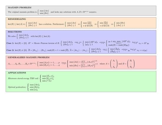
Graphical Abstract

1. Introduction

1.1. Scope

Different scientific fields, such as Physics, Statistics, Economics, or Engineering, deal with real-life problems that are usually modelled by the experts on those fields using matrices and their norms (see [1,2,3,4,5,6]). A typical modelling is the following original maxmin problem
max A x min B x .
One of the most iconic results in this manuscript (Theorem 2) shows that the previous problem, regarded strictly as a multiple optimization problem, has no solutions. To save this obstacle we provide a different model, such as
max A x B x 1 .
Here in this article we justify the remodelling of the original maxmin problem and we solve it by making use of supporting vectors. This concept comes from the Theory of Banach Spaces and Operator Theory. Given a matrix A, a supporting vector is a unit vector x such that A attains its norm at x, that is, x is a solution of the following single optimization problem:
max A x x = 1 .
The geometric and topological structure of supporting vectors can be consulted in [7,8,9]. On the other hand, generalized supporting vectors are defined and studied in [7,8]. The generalized supporting vectors of a finite sequence of matrices A 1 , , A n , for the Euclidean norm 2 , are the solutions of
max A 1 x 2 2 + + A n x 2 2 x 2 = 1 .
This optimization problem clearly generalizes the previous one.
Supporting vectors were originally applied in [10] to truly optimally design a TMS coil, because until that moment TMS coils had only been designed by means of heuristic methods, which were never proved to be convergent. In [10] a three-component TMS coil problem is posed but only the one-component case was resolved. The three-component case was stated and solved by means of the generalized supporting vectors in [8]. In this manuscript, we model a TMS coil with a maxmin problem and solve it exactly with our method.
A second application of supporting vectors was given in [8], where an optimal location situation using Principal Component Analysis (PCA) was solved. In this manuscript, we model a more complex PCA problem as an optimal maxmin geolocation involving statistical variables.
For other perspective on supporting vectors and generalized supporting vectors, we refer the reader to [9].

1.2. Background

In the first place, we refer the reader to [8] (Preliminaries) for a general review of multiobjective optimization problems and their reformulations to avoid the lack of solutions (generally caused by the existence of many objective functions).
The original maxmin optimization problem has the form
M : = max g ( x ) min f ( x )
where f , g : X ( 0 , ) are real-valued functions and X is a nonempty set. Notice that
sol ( M ) = arg max g ( x ) arg min f ( x ) .
Many real-life problems can be mathematically model, such as a maxmin. However, this kind of multiobjective optimization problems may have the inconvenience of lacking a solution. If this occurs, then we are in need of remodeling the real-life problem with another mathematical optimization problem that has a solution and still models the real-life problem very accurately.
According to [10] (Theorem 5.1), one can realize that, in case sol ( M ) = , the following optimization problems are good alternatives to keep modeling the real-life problem accurately:
  • max g ( x ) min f ( x ) reform min f ( x ) g ( x ) g ( x ) 0 .
  • max g ( x ) min f ( x ) reform max g ( x ) f ( x ) f ( x ) 0 .
  • max g ( x ) min f ( x ) reform max g ( x ) f ( x ) a .
  • max g ( x ) min f ( x ) reform min f ( x ) g ( x ) b .
We will prove in the third section that all four previous reformulations are equivalent for the original maxmin max A x min B x . In the fourth section, we will solve the reformulation max A x B x 1 .

2. Characterizations of Operators with Null Kernel

Kernels will play a fundamental role towards solving the general reformulated maxmin (2) as shown in the next section. This is why we first study the operators with null kernel.
Throughout this section, all monoid actions considered will be left, all rings will be associative, all rings will be unitary rngs, all absolute semi-values and all semi-norms will be non-zero, all modules over rings will be unital, all normed spaces will be real or complex and all algebras will be unitary and complex.
Given a rng R and an element s R , we will denote by d ( s ) to the set of left divisors of s, that is,
d ( s ) : = { r R : t R { 0 } with r t = s } .
Similarly, rd ( s ) stands for the set of right divisors of s. If R is a ring, then the set of its invertibles is usually denoted by U ( R ) . Notice that d ( 1 ) ( rd ( 1 ) ) is precisely the subset of elements of R which are right-(left) invertible. As a consequence, U ( R ) = d ( 1 ) rd ( 1 ) . Observe also that d ( 0 ) rd ( 1 ) = = rd ( 0 ) d ( 1 ) . In general we have that d ( 0 ) d ( 1 ) and rd ( 0 ) rd ( 1 ) . Later on in Example 1 we will provide an example of a ring where rd ( 0 ) rd ( 1 ) .
Recall that an element p of a monoid is called involutive if p 2 = 1 . Given a rng R, an involution is an additive, antimultiplicative, composition-involutive map : R R . A -rng is a rng endowed with an involution.
The categorical concept of monomorphism will play an important role in this manuscript. A morphism f hom C ( A , B ) between objects A and B in a category C is said to be a monomorphism provided that f g = f h implies g = h for all C ob ( C ) and all g , h hom C ( C , A ) . Once can check that if f hom C ( A , B ) and there exist C 0 ob ( C ) and g 0 hom C ( B , C 0 ) such that g 0 f is a monomorphism, then f is also a monomorphism. In particular, if f hom C ( A , B ) is a section, that is, exists g hom C ( B , A ) such that g f = I A , then f is a monomorphism. As a consequence, the elements of hom C ( A , A ) that have a left inverse are monomorphisms. In some categories, the last condition suffices to characterize monomorphisms. This is the case, for instance, of the category of vector spaces over a division ring.
Recall that CL ( X , Y ) denotes the space of continuous linear operators from a topological vector space X to another topological vector space Y.
Proposition 1.
A continuous linear operator T : X Y between locally convex Hausdorff topological vector spaces X and Y verifies that ker ( T ) { 0 } if and only if exists S CL ( Y , X ) { 0 } with T S = 0 . In particular, if X = Y , then ker ( T ) { 0 } if and only if T d ( 0 ) in CL ( X ) .
Proof. 
Let S CL ( Y , X ) { 0 } such that T S = 0 . Fix any y Y ker ( S ) , then S ( y ) 0 and T ( S ( y ) ) = 0 so S ( y ) ker ( T ) { 0 } . Conversely, if ker ( T ) { 0 } , then fix x 0 ker ( T ) { 0 } and y 0 Y { 0 } (the existence of y is guaranteed by the Hahn-Banach Theorem on the Hausdorff locally convex topological vector space Y). Next, consider
S : Y X y S ( y ) : = y 0 ( y ) x 0 .
Notice that S CL ( Y , X ) { 0 } and T S = 0 . □
Theorem 1.
Let T : X Y be a continuous linear operator between locally convex Hausdorff topological vector spaces X and Y. Then:
1. 
If T is a section, then ker ( T ) = { 0 }
2. 
In case X and Y are Banach spaces, T ( X ) is topologically complemented in Y and ker ( T ) = { 0 } , then T is a section.
Proof. 
  • Trivial since sections are monomorphisms.
  • Consider T : X T ( X ) . Since T ( X ) is topologically complemented in Y we have that T ( X ) is closed in Y, thus it is a Banach space. Therefore, the Open Mapping Theorem assures that T : X T ( X ) is an isomorphism. Let T 1 : T ( X ) X be the inverse of T : X T ( X ) . Now consider P : Y Y to be a continuous linear projection such that P ( Y ) = T ( X ) . Finally, it suffices to define S : = T 1 P since S T = I X .
 □
We will finalize this section with a trivial example of a matrix A R 3 × 2 such that A rd ( I ) rd ( 0 ) .
Example 1.
Consider
A = 1 0 0 1 0 0 .
It is not hard to check that ker ( A ) = { ( 0 , 0 ) } thus A is left-invertible by Theorem 1(2) and so A rd ( I ) . In fact,
1 0 0 0 1 0 1 0 0 1 0 0 = 1 0 0 1 .
Finally,
0 0 1 0 0 1 1 0 0 1 0 0 = 0 0 0 0 .

3. Remodeling the Original Maxmin Problem max T ( x ) Subject to min S ( x )

3.1. The Original Maxmin Problem Has No Solutions

This subsection begins with the following theorem:
Theorem 2.
Let T , S : X Y be nonzero continuous linear operators between Banach spaces X and Y. Then the original maxmin problem
max T ( x ) min S ( x )
has trivially no solution.
Proof. 
Observe that arg min S ( x ) = ker ( S ) and arg max T ( x ) = because T { 0 } . Then the set of solutions of Problem (1) is
arg min S ( x ) arg max T ( x ) = ker ( S ) = .
 □
As a consequence, Problem (1) must be reformulated or remodeled.

3.2. Equivalent Reformulations for the Original Maxmin Problem

According to the Background section, we begin with the following reformulation:
max T ( x ) S ( x ) 1
Please note that arg max S ( x ) 1 T ( x ) is a K -symmetric set, where K : = R or C , in other words, if λ K and | λ | = 1 , then λ x arg max S ( x ) 1 T ( x ) for every x arg max S ( x ) 1 T ( x ) . The finite dimensional version of the previous reformulation is
max A x B x 1
where A , B R m × n .
Recall that B ( X , Y ) denotes the space of bounded operators from X to Y.
Lemma 1.
Let T , S B ( X , Y ) where X and Y are Banach spaces. If the general reformulated maxmin problem
max T ( x ) S ( x ) 1
has a solution, then ker ( S ) ker ( T ) .
Proof. 
If ker ( S ) ker ( T ) , then it suffices to consider the sequence ( n x 0 ) n N for x 0 ker ( S ) ker ( T ) , since S ( n x 0 ) = 0 1 for all n N and T ( n x 0 ) = n T ( x 0 ) as n . □
The general maxmin (1) can also be reformulated as
max T ( x ) min S ( x ) reform max T ( x ) S ( x ) S ( x ) 0
Lemma 2.
Let T , S B ( X , Y ) where X and Y are Banach spaces. If the second general reformulated maxmin problem
max T ( x ) S ( x ) S ( x ) 0
has a solution, then ker ( S ) ker ( T ) .
Proof. 
Suppose there exists x 0 ker ( S ) ker ( T ) . Then fix an arbitrary x 1 X ker ( S ) . Notice that
T ( n x 0 + x 1 ) S ( n x 0 + x 1 ) n T ( x 0 ) T ( x 1 ) S ( x 1 )
as n . □
The next theorem shows that the previous two reformulations are in fact equivalent.
Theorem 3.
Let T , S B ( X , Y ) where X and Y are Banach spaces. Then
t > 0 t arg max S ( x ) 1 T ( x ) = arg max S ( x ) 0 T ( x ) S ( x ) .
Proof. 
Let x 0 arg max S ( x ) 1 T ( x ) and t 0 > 0 . Fix an arbitrary y X ker ( S ) . Notice that x 0 ker ( S ) in virtue of Theorem 1. Then
T ( x 0 ) T y S ( y ) ,
therefore
T ( t x 0 ) S ( t x 0 ) = T ( x 0 ) S ( x 0 ) T ( x 0 ) T y S ( y ) .
Conversely, let x 0 arg max S ( x ) 0 T ( x ) S ( x ) . Fix an arbitrary y X with S ( y ) 1 . Then
T x 0 S ( x 0 ) = T ( x 0 ) S ( x 0 ) T ( y ) S ( y ) T ( y )
which means that
x 0 S ( x 0 ) arg max S ( x ) 1 T ( x )
and thus
x 0 S ( x 0 ) arg max S ( x ) 1 T ( x ) t > 0 t arg max S ( x ) 1 T ( x ) .
 □
The reformulation
min S ( x ) T ( x ) T ( x ) 0
is slightly different from the previous two reformulations. In fact, if ker ( S ) ker ( T ) , then arg min T ( x ) 0 S ( x ) T ( x ) = ker ( S ) ker ( T ) . The previous reformulation is equivalent to the following one as shown in the next theorem:
min S ( x ) T ( x ) 1
Theorem 4.
Let T , S B ( X , Y ) where X and Y are Banach spaces. Then
t > 0 t arg min T ( x ) 1 S ( x ) = arg min T ( x ) 0 S ( x ) T ( x ) .
We spare of the details of the proof of the previous theorem to the reader. Notice that if ker ( S ) ker ( T ) , then arg min T ( x ) 1 S ( x ) = ker ( S ) { x : T ( x ) < 1 } . However, if ker ( S ) ker ( T ) , then all four reformulations are equivalent, as shown in the next theorem, whose proof’s details we spare again to the reader.
Theorem 5.
Let T , S B ( X , Y ) where X and Y are Banach spaces. If ker ( S ) ker ( T ) , then
arg max S ( x ) 0 T ( x ) S ( x ) = arg min T ( x ) 0 S ( x ) T ( x ) .

4. Solving the Maxmin Problem max T ( x ) Subject to S ( x ) 1

We will distinguish between two cases.

4.1. First Case: S Is an Isomorphism Over Its Image

By bearing in mind Theorem 5, we can focus on the first reformulation proposed at the beginning of the previous section:
max T ( x ) min S ( x ) reform max T ( x ) S ( x ) 1
The idea we propose to solve the previous reformulation is to make use of supporting vectors (see [7,8,9,10]). Recall that if R : X Y is a continuous linear operator between Banach spaces, then the set of supporting vectors of R is defined by
suppv ( R ) : = arg max x 1 R ( x ) .
The idea of using supporting vectors is that the optimization problem
max R ( x ) x 1
whose solutions are by definition the supporting vectors of R, can be easily solved theoretically and computationally (see [8]).
Our first result towards this direction considers the case where S is an isomorphism over its image.
Theorem 6.
Let T , S B ( X , Y ) where X and Y are Banach spaces. Suppose that S is an isomorphism over its image and S 1 : S ( X ) X denotes its inverse. Suppose also that S ( X ) is complemented in Y, being p : Y Y a continuous linear projection onto S ( X ) . Then
S 1 S ( X ) arg max y 1 T S 1 p ( y ) arg max S ( x ) 1 T ( x ) .
If, in addition, p = 1 , then
arg max S ( x ) 1 T ( x ) = S 1 S ( X ) arg max y 1 T S 1 p ( y ) .
Proof. 
We will show first that
S ( X ) arg max y 1 T S 1 p ( y ) S arg max S ( x ) 1 T ( x ) .
Let y 0 = S ( x 0 ) arg max y 1 T S 1 p ( y ) . We will show that x 0 arg max S ( x ) 1 T ( x ) . Indeed, let x X with S ( x ) 1 . Since S ( x 0 ) = y 0 1 , by assumption we obtain
T ( x ) = T S 1 p ( S ( x ) ) T S 1 p ( y 0 ) = T S 1 p ( S ( x 0 ) ) = T ( x 0 ) .
Now assume that p = 1 . We will show that
S arg max S ( x ) 1 T ( x ) S ( X ) arg max y 1 T S 1 p ( y ) .
Let x 0 arg max S ( x ) 1 T ( x ) , we will show that S ( x 0 ) arg max y 1 T S 1 p ( y ) . Indeed, let y B Y . Observe that
S S 1 ( p ( y ) ) = p ( y ) y 1
so by assumption
T S 1 p ( y ) = T S 1 ( p ( y ) ) T ( x 0 ) = T S 1 ( p ( S ( x 0 ) ) ) = T S 1 p ( S ( x 0 ) ) .
 □
Notice that, in the settings of Theorem 6, S 1 p is a left-inverse of S, in other words, S is a section, as in Theorem 1(2).
Taking into consideration that every closed subspace of a Hilbert space is 1-complemented (see [11,12] to realize that this fact characterizes Hilbert spaces of dimension 3 ), we directly obtain the following corollary.
Corollary 1.
Let T , S B ( X , Y ) where X is a Banach space and Y a Hilbert space. Suppose that S is an isomorphism over its image and let S 1 : S ( X ) X be its inverse. Then
arg max S ( x ) 1 T ( x ) = S 1 S ( X ) arg max y 1 T S 1 p ( y ) = S 1 S ( X ) suppv T S 1 p
where p : Y Y is the orthogonal projection on S ( X ) .

4.2. The Moore–Penrose Inverse

If B K m × n , then the Moore–Penrose inverse of B, denoted by B + , is the only matrix B + K n × m which verifies the following:
  • B = B B + B .
  • B + = B + B B + .
  • B B + = ( B B + ) .
  • B + B = ( B + B ) .
If ker ( B ) = 0 , then B + is a left-inverse of B. Even more, B B + is the orthogonal projection onto the range of B, thus we have the following result from Corollary 1.
Corollary 2.
Let A , B R m × n such that ker ( B ) = { 0 } . Then
B arg max B x 2 1 A x 2 = B R n arg max y 2 1 A B + y 2 = B R n suppv A B +
According to the previous Corollary, in its settings, if y 0 arg max y 2 1 A B + y 2 and there exists x 0 R n such that y 0 = B x 0 , then x 0 arg max B x 2 1 A x 2 and x 0 can be computed as
x 0 = B + B x 0 = B + y 0 .

4.3. Second Case: S Is Not an Isomorphism Over Its Image

What happens if S is not an isomorphism over its image? Next theorem answers this question.
Theorem 7.
Let T , S B ( X , Y ) where X and Y are Banach spaces. Suppose that ker ( S ) ker ( T ) . If
π : X X / ker ( S ) x π ( x ) : = x + ker ( S )
denotes the quotient map, then
arg max S ( x ) 1 T ( x ) = π 1 arg max S ¯ ( π ( x ) ) 1 T ¯ ( π ( x ) ) ,
where
T ¯ : X ker ( S ) Y π ( x ) T ¯ ( π ( x ) ) : = T ( x )
and
S ¯ : X ker ( S ) Y π ( x ) S ¯ ( π ( x ) ) : = S ( x ) .
Proof. 
Let x 0 arg max S ( x ) 1 T ( x ) . Fix an arbitrary y X with S ¯ ( π ( y ) ) 1 . Then S ( y ) = S ¯ ( π ( y ) ) 1 therefore
T ¯ ( π ( x 0 ) = T ( x 0 ) T ( y ) = T ¯ ( π ( y ) ) .
This shows that π ( x 0 ) arg max S ¯ ( π ( x ) ) 1 T ¯ ( π ( x ) ) . Conversely, let
π ( x 0 ) arg max S ¯ ( π ( x ) ) 1 T ¯ ( π ( x ) ) .
Fix an arbitrary y X with S ( y ) 1 . Then S ¯ ( π ( y ) ) = S ( y ) 1 therefore
T ( x 0 ) = T ¯ ( π ( x 0 ) ) T ¯ ( π ( y ) ) = T ( y ) .
This shows that x 0 arg max S ( x ) 1 T ( x ) . □
Please note that in the settings of Theorem 7, if S ( X ) is closed in Y, then S ¯ is an isomorphism over its image S ( X ) , and thus in this case Theorem 7 reduces the reformulated maxmin to Theorem 6.

4.4. Characterizing When the Finite Dimensional Reformulated Maxmin Has a Solution

The final part of this section is aimed at characterizing when the finite dimensional reformulated maxmin has a solution.
Lemma 3.
Let S : X Y be a bounded operator between finite dimensional Banach spaces X and Y. If ( x n ) n N is a sequence in { x X : S ( x ) 1 } , then there is a sequence ( z n ) n N in ker ( S ) so that ( x n + z n ) n N is bounded.
Proof. 
Consider the linear operator
S ¯ : X ker ( S ) Y x + ker ( S ) S ¯ ( x + ker ( S ) ) = S ( x ) .
Please note that
S ¯ ( x n + ker ( S ) ) = S ( x n ) 1
for all n N , therefore the sequence ( x n + ker ( S ) ) n N is bounded in X ker ( S ) because X ker ( S ) is finite dimensional and S ¯ has null kernel so its inverse is continuous. Finally, choose z n ker ( S ) such that x n + z n < x n + ker ( S ) + 1 n for all n N . □
Lemma 4.
Let A , B R m × n . If ker ( B ) ker ( A ) , then A is bounded on { x R n : B x 1 } and attains its maximum on that set.
Proof. 
Let ( x n ) n N be a sequence in { x R n : B x 1 } . In accordance with Lemma 3, there exists a sequence ( z n ) n N in ker ( B ) such that ( x n + z n ) n N is bounded. Since A ( x n ) = A ( x n + z n ) by hypothesis (recall that ker ( B ) ker ( A ) ), we conclude that A is bounded on { x R n : B x 1 } . Finally, let ( x n ) n N be a sequence in { x R n : B x 1 } such that A x n max B x 1 A x as n . Please note that A ¯ ( x n + ker ( B ) ) = A x n for all n N , so A ¯ ( x n + ker ( B ) ) n N is bounded in R m and so is A ¯ ( x n + ker ( B ) ) n N in R n ker ( B ) . Fix b n ker ( B ) such that x n + b n < x n + ker ( B ) + 1 n for all n N . This means that ( x n + b n ) n N is a bounded sequence in R n so we can extract a convergent subsequence x n k + b n k k N to some x 0 X . At this stage, notice that B x n k + b n k = B x n k 1 for all k N and B x n k + b n k k N converges to B x 0 , so B x 0 1 . Note also that, since ker ( B ) ker ( A ) , A x n k n N converges to A x 0 , which implies that
x 0 arg max B x 1 A x .
 □
Theorem 8.
Let A , B R m × n . The reformulated maxmin problem
max A x B x 1
has a solution if and only if ker ( B ) ker ( A ) .
Proof. 
If ker ( B ) ker ( A ) , then we just need to call on Lemma 4. Conversely, if ker ( B ) ker ( A ) , then it suffices to consider the sequence ( n x 0 ) n N for x 0 ker ( B ) ker ( A ) , since B ( n x 0 ) = 0 1 for all n N and A ( n x 0 ) = n A ( x 0 ) as n . □

4.5. Matrices on Quotient Spaces

Consider the maxmin
max T ( x ) S ( x ) 1
being X and Y Banach spaces and T , S B ( X , Y ) with ker ( S ) ker ( T ) . Notice that if ( e i ) i I is a Hamel basis of X, then e i + ker ( S ) i I is a generator system of X ker ( S ) . By making use of the Zorn’s Lemma, it can be shown that e i + ker ( S ) i I contains a Hamel basis of X ker ( S ) . Observe that a subset C of X ker ( S ) is linearly independent if and only if S ( C ) is a linearly independent subset of Y.
In the finite dimensional case, we have
B ¯ : R n ker ( B ) R m x + ker ( B ) B ¯ ( x + ker ( B ) ) : = B x .
and
A ¯ : R n ker ( B ) R m x + ker ( B ) A ¯ ( x + ker ( B ) ) : = A x .
If { e 1 , , e n } denotes the canonical basis of R n , then { e 1 + ker ( B ) , , e n + ker ( B ) } is a generator system of R n ker ( B ) . This generator system contains a basis of R n ker ( B ) so let { e j 1 + ker ( B ) , , e j l + ker ( B ) } be a basis of R n ker ( B ) . Please note that A ¯ e j k + ker ( B ) = A e j k and B ¯ e j k + ker ( B ) = B e j k for every k { 1 , , l } . Therefore, the matrix associated with the linear map defined by B ¯ can be obtained from the matrix B by removing the columns corresponding to the indices { 1 , , n } { j 1 , , j l } , in other words, the matrix associated with B ¯ is B e j 1 | | B e j l . Similarly, the matrix associated with the linear map defined by A ¯ is A e j 1 | | A e j l . As we mentioned above, recall that a subset C of R n ker ( B ) is linearly independent if and only if B ( C ) is a linearly independent subset of R m . As a consequence, in order to obtain the basis { e j 1 + ker ( B ) , , e j l + ker ( B ) } , it suffices to look at the rank of B and consider the columns of B that allow such rank, which automatically gives us the matrix associated with B ¯ , that is, B e j 1 | | B e j l .
Finally, let
π : R n R n ker ( B ) x π ( x ) : x + ker ( B )
denote the quotient map. Let l : = rank ( B ) = dim R n ker ( B ) . If x = ( x 1 , , x l ) R l , then k = 1 l x k e j k + ker ( B ) R n ker ( B ) . The vector z R n defined by
z p : = x k p = j k 0 p { j 1 , , j l }
verifies that
p ( z ) = k = 1 l x k e j k + ker ( B ) .
To simplify the notation, we can define the map
α : R l R n x α ( x ) : = z
where z is the vector described right above.
5. Discussion

Here we compile all the results from the previous subsections and define the structure of the algorithm that solves the maxmin (3).
Let A , B R m × n with ker ( B ) ker ( A ) . Then
max A x 2 min B x 2 reform max A x 2 B x 2 1
Case 1:
ker ( B ) = { 0 } . B + denotes the Moore–Penrose inverse of B.
max A x 2 B x 2 1 supp . vec . max A B + y 2 y 2 1 solution y 0 arg max y 2 1 A B + y 2 rank ( B ) = rank ( [ B | y 0 ] ) final sol . x 0 : = B + y 0
Case 2:
ker ( B ) { 0 } . B ¯ = B e j 1 | | B e j l where rank ( B ) = l = rank B ¯ and A ¯ = A e j 1 | | A e j l .
max A x 2 B x 2 1 case 1 max A ¯ y 2 B ¯ y 2 1 solution y 0 final sol . x 0 : = α ( y 0 )
In case a real-life problem is modeled like a maxmin involving more operators, we proceed as the following remark establishes in accordance with the preliminaries of this manuscript (reducing the number of multiobjective functions to avoid the lack of solutions):
Remark 1.
Let ( T n ) n N and ( S n ) n N be sequences of continuous linear operators between Banach spaces X and Y. The maxmin
max T n ( x ) n N min S n ( x ) n N
can be reformulated as (recall the second typical reformulation)
max n = 1 T n ( x ) 2 min n = 1 S n ( x ) 2
which can be transformed into a regular maxmin as in (1) by considering the operators
T : X 2 ( Y ) x T ( x ) : = ( T n ( x ) ) n N
and
S : X 2 ( Y ) x S ( x ) : = ( S n ( x ) ) n N
obtaining then
max T ( x ) 2 min S ( x ) 2
which is equivalent to
max T ( x ) min S ( x )
Observe that for the operators T and S to be well defined it is sufficient that ( T n ) n N and ( S n ) n N be in 2 .

6. Materials and Methods

The initial methodology employed in this research work is the Mathematical Modelling of real-life problems. The subsequent methodology followed is given by the Axiomatic-Deductive Method framed in the First-Order Mathematical language. Inside this framework, we deal with the Category Theory (the main category involved is the Category of Banach spaces with the Bounded Operators). The final methodology used is the implementation of our mathematical results in the MATLAB programming language.

7. Conclusions

We finally enumerate the novelties provided in this work, which serve as conclusions for our research:
  • We prove that the original maxmin problem
    max A x min B x
    has no solution (Theorem 2).
  • We then rewrite (6) as
    max A x B x 1
    which still models the real-life problem very accurately and has a solution if and only if ker ( B ) ker ( A ) (Theorem 8).
  • We provide an exact solution of (7) assuming ker ( B ) ker ( A ) , not an heuristic method for approaching it. See Section 5.
  • A MATLAB code is provided for computing the solution to the maxmin problem. See Appendix C.
  • Our solution applies to design truly optimal minimum stored-energy TMS coils and to find more complex optimal geolocations involving statistical variables. See Appendixes Appendix A and Appendix B.
  • This article represents an interdisciplinary work involving pure abstract nontrivial proven theorems and programming codes that can be directly applied to different situations in the real world.

Author Contributions

Conceptualization, S.M.-P., F.J.G.-P., C.C.-S. and A.S.-A.; methodology, S.M.-P., F.J.G.-P., C.C.-S. and A.S.-A.; software, S.M.-P., F.J.G.-P., C.C.-S. and A.S.-A.; validation, S.M.-P., F.J.G.-P., C.C.-S. and A.S.-A.; formal analysis, S.M.-P., F.J.G.-P., C.C.-S. and A.S.-A.; investigation, S.M.-P., F.J.G.-P., C.C.-S. and A.S.-A.; resources, S.M.-P., F.J.G.-P., C.C.-S. and A.S.-A.; data curation, S.M.-P., F.J.G.-P., C.C.-S. and A.S.-A.; writing—original draft preparation, S.M.-P., F.J.G.-P., C.C.-S. and A.S.-A.; writing—review and editing, S.M.-P., F.J.G.-P., C.C.-S. and A.S.-A.; visualization, S.M.-P., F.J.G.-P., C.C.-S. and A.S.-A.; supervision, S.M.-P., F.J.G.-P., C.C.-S. and A.S.-A.; project administration, S.M.-P., F.J.G.-P., C.C.-S. and A.S.-A.; funding acquisition, S.M.-P., F.J.G.-P., C.C.-S. and A.S.-A. All authors have read and agreed to the published version of the manuscript.

Funding

This research was funded by the Research Grant PGC-101514-B-100 awarded by the Spanish Ministry of Science, Innovation and Universities and partially funded by FEDER.

Conflicts of Interest

The authors declare no conflict of interest. The funders had no role in the design of the study; in the collection, analyses, or interpretation of data; in the writing of the manuscript, or in the decision to publish the results.

Appendix A. Applications to Optimal TMS Coils

Appendix A.1. Introduction to TMS Coils

Transcranial Magnetic Stimulation (TMS) is a non-invasive technique to stimulate the brain. We refer the reader to [8,10,13,14,15,16,17,18,19,20,21,22,23] for a description on the development of TMS coils desing as an optimization problem.
An important safety issue in TMS is the minimization of the stimulation of non-target areas. Therefore, the development of TMS as a medical tool would be benefited with the design of TMS stimulators capable of inducing a maximum electric field in the region of interest, while minimizing the undesired stimulation in other prescribed regions.

Appendix A.2. Minimum Stored-Energy TMS Coil

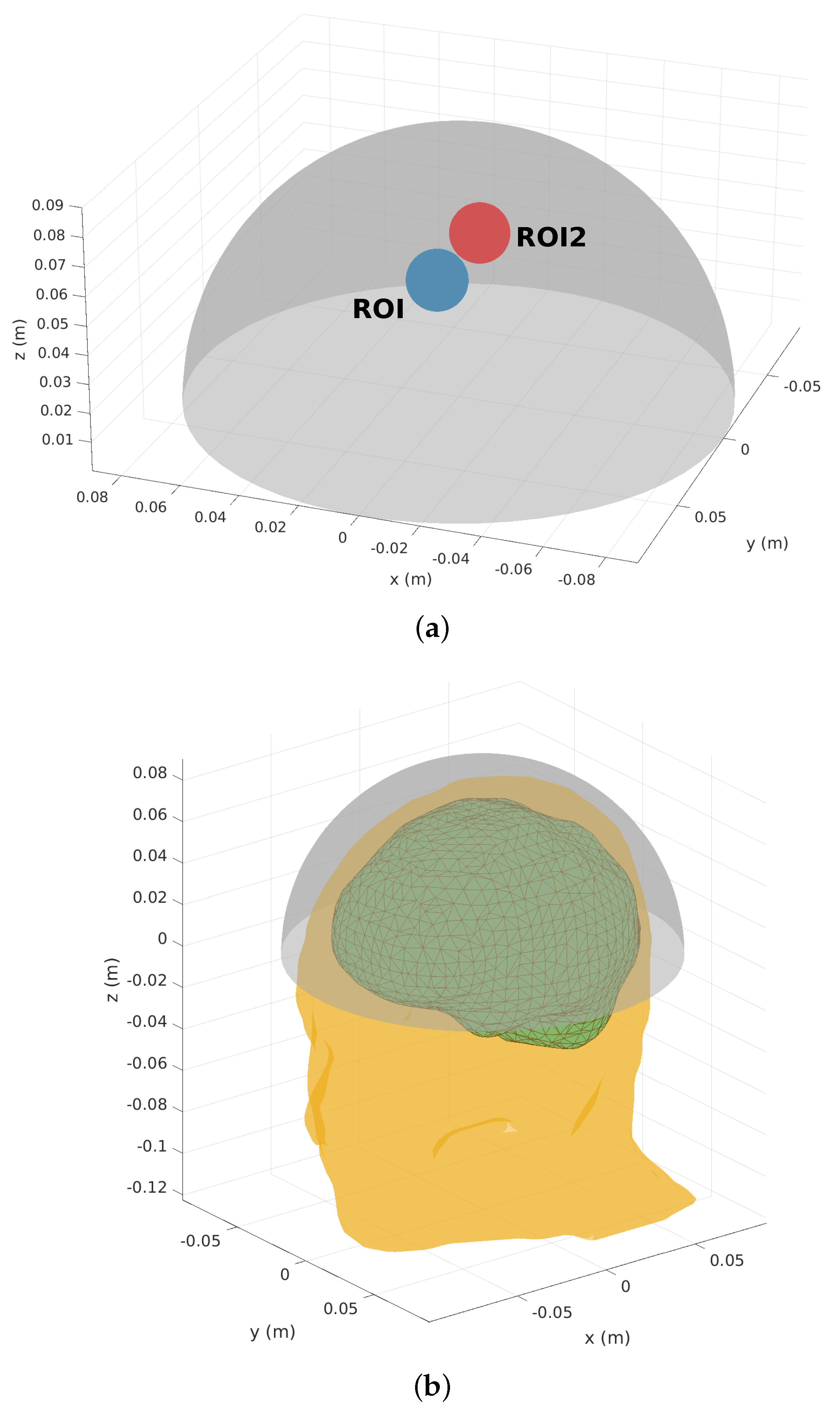
In the following section, in order to illustrate an application of the theoretical model developed in this manuscript, we are going to tackle the design of a minimum stored-energy hemispherical TMS coil of radius 9 cm, constructed to stimulate only one cerebral hemisphere. To this end, the coil must produce an E-field which is both maximum in a spherical region of interest (ROI) and minimum in a second region (ROI2). Both volumes of interest are of 1 cm radius and formed by 400 points, where ROI is shifted by 5 cm in the positive z-direction and by 2 cm in the positive y-direction; and ROI2 is shifted by 5 cm in the positive z-direction and by 2 cm in the negative y-direction, as shown in Figure A1a. In Figure A1b a simple human head made of two compartments, scalp and brain, used to evaluate the performance of the designed stimulator is shown.
Figure A1. (a) Description of hemispherical surface where the optimal ψ must been found along with the spherical regions of interest ROI and ROI2 where the electric field must be maximized and minimized respectively. (b) Description of the two compartment scalp-brain model.
Mathematics 08 00085 g0a1
By using the formalism presented in [10] this TMS coil design problem can be posed as the following optimization problem:
max E x 1 ψ 2 min E x 2 ψ 2 min ψ T L ψ
where ψ is the stream function (the optimization variable), M = 400 are the number of points in the ROI and ROI2, N = 2122 the number of mesh nodes, L R N × N is the inductance matrix, and E x 1 R M × N and E x 2 R M × N are the E-field matrices in the prescribe x-direction.
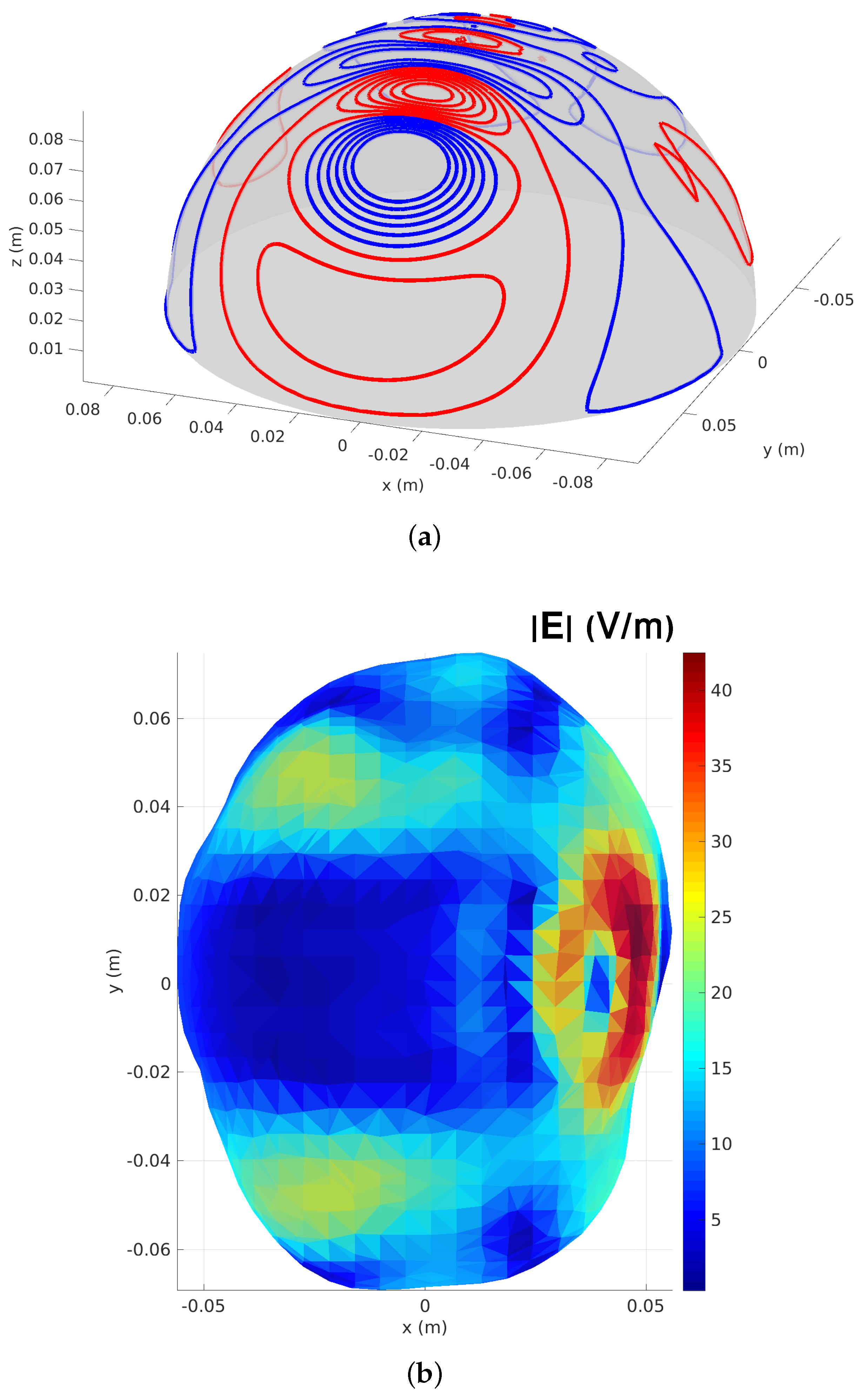
Figure A2. (a) Wirepaths with 18 turns of the TMS coil solution (red wires indicate reversed current flow with respect to blue). (b) E-field modulus induced at the surface of the brain by the designed TMS coil.
Mathematics 08 00085 g0a2
Figure A2a shows the coil solution of problem in Equation (A1) computed by using the theoretical model proposed in this manuscript (see Section 5 and Appendix A.3), and as expected, the wire arrangements is remarkably concentrated over the region of stimulation.
To evaluate the stimulation of the coil, we resort to the direct BEM [24], which permits the computation of the electric field induced by the coils in conducting systems. As can be seen in Figure A2b, the TMS coil fulfils the initial requirements of stimulating only one hemisphere of the brain (the one where ROI is found); whereas the electric field induced in the other cerebral hemisphere (where ROI2 can be found) is minimum.

Appendix A.3. Reformulation of Problem (A1) to Turn it into a Maxmin

Now it is time to reformulate the multiobjective optimization problem given in (A1), because it has no solution in virtue of Theorem 2. We will transform it into a maxmin problem as in (7) so that we can apply the theoretical model described in Section 5:
max E x 1 ψ 2 min E x 2 ψ 2 min ψ T L ψ
Since raising to the square is a strictly increasing function on [ 0 , ) , the previous problem is trivially equivalent to the following one:
max E x 1 ψ 2 2 min E x 2 ψ 2 2 min ψ T L ψ
Next, we apply Cholesky decomposition to L to obtain L = C T C so we have that ψ T L ψ = ( C ψ ) T ( C ψ ) = C ψ 2 2 so we obtain
max E x 1 ψ 2 2 min E x 2 ψ 2 2 min C ψ 2 2
Since C is an invertible square matrix, arg min C ψ 2 2 = { 0 } so the previous multiobjective optimization problem has no solution. Therefore it must be reformulated. We call then on Remark 1 to obtain:
max E x 1 ψ 2 2 min E x 2 ψ 2 2 + C ψ 2 2
which in essence is
max E x 1 ψ 2 min D ψ 2
where D : = E x 2 C . The matrix D in this specific case has null kernel. In accordance with the previous sections, Problem (A5) is remodeled as
max E x 1 ψ 2 D ψ 2 1
Finally, we can refer to Section 5 to solve the latter problem.

Appendix B. Applications to Optimal Geolocation

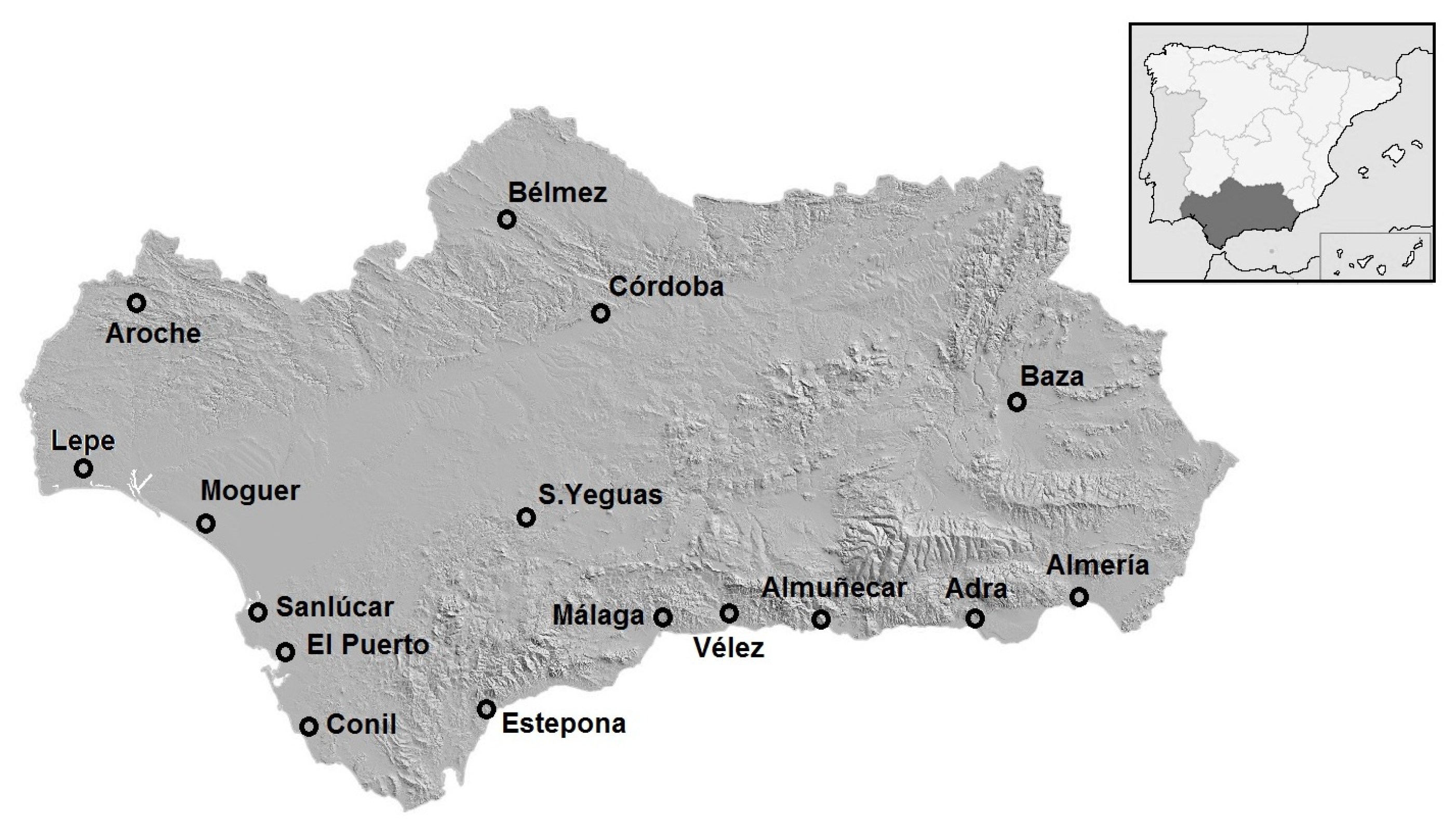
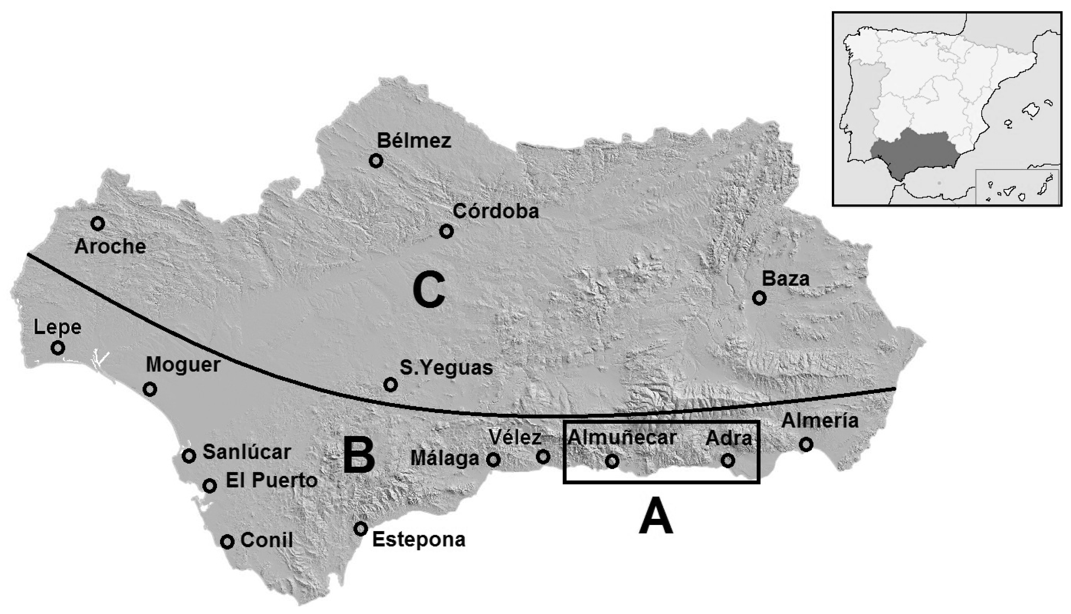
Several studies involving optimal geolocation [25], multivariate statistics [26,27] and multiobjective problems [28,29,30] were carried out recently. To show another application of maxmin multiobjective problems, we consider in this work the best situation of a tourism rural inn considering several measured climate variables. Locations with low highest temperature m 1 , radiation m 2 and evapotranspiration m 3 in summer time and high values in winter time are sites with climatic characteristics desirable for potential visitors. To solve this problem, we choose 11 locations in the Andalusian coastline and 2 in the inner, near the mountains. We have collected the data from the official Andalusian government webpage [31] evaluating the mean values of these variables on the last 5 years 2013–2019. The referred months of the study were January and July.
Table A1. Mean values of high temperature (T) in Celsius Degrees, radiation (R) in M J / m 2 , and evapotranspiration (E) in mm/day, measures in January (winter time) and July (summer time) between 2013 and 2018.
T-WinterR-WinterE-WinterT-SummerR-SummerE-Summer
Sanlúcar15.9599.5721.52030.08627.7586.103
Moguer16.6989.2720.92530.42427.7515.222
Lepe16.6599.5031.24230.61028.2976.836
Conil16.3229.9401.33128.91326.6695.596
El Puerto16.5049.7671.62531.05228.2166.829
Estepona16.90810.1941.77331.23327.2986.246
Málaga17.6639.9681.60632.35827.5286.378
Vélez18.2049.8191.90531.91226.5345.911
Almuñécar17.73310.2471.40429.68425.3704.952
Adra17.78410.1981.63728.92926.4635.143
Almería17.46810.0681.56130.34227.3355.793
Aroche16.4779.7971.43434.61627.8066.270
Córdoba14.8718.9521.14936.37528.5037.615
Baza13.3868.3033.05435.75427.8241.673
Bélmez13.1508.2161.21535.27228.4787.400
S. Yeguas13.6569.1551.24733.66028.7277.825
To find the optimal location, let us evaluate the site where the variables mean values are maximum in January and minimum in July. Here we have a typical multiobjective problem with two data matrices that can be formulated as follows:
max A x 2 min B x 2 min x 2
where A and B are real 16 × 3 matrices with the values of the three variables ( m 1 , m 2 , m 3 ) taking into account (highest temperature, radiation and evapotranspiration) in January and July respectively. To avoid unit effects, we standarized the variables ( μ = 0 and σ = 1 ). The vector x is the solution of the multiobjective problem.
Since (A7) lacks any solution in view of Theorem 2, we reformulate it as we showed in Remark 1 by the following:
max A x 2 min D x 2
with matrix D : = B I n , where I n is the identity matrix with n = 3 . Notice that it also verifies that ker ( D ) = { 0 } . Observe that, according to the previous sections, (A8) can be remodeled into
max A x 2 D x 2 1
and solved accordingly.
Figure A3. Geographic distribution of the sites considered in the study. 11 places are in the coastline of the region and 5 in the inner.
Mathematics 08 00085 g0a3
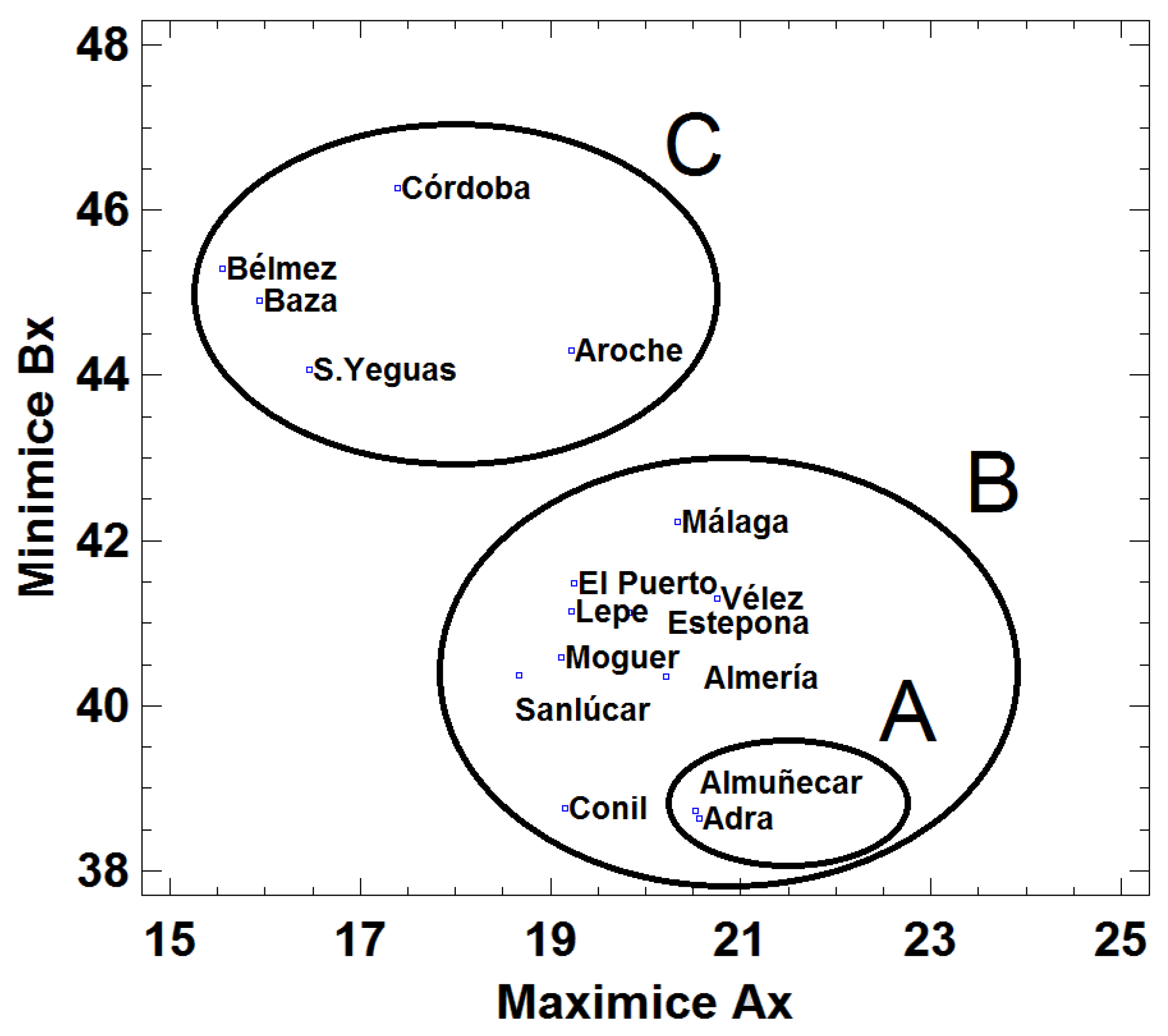
Figure A4. Locations considering Ax and Bx axes. Group named A represents the best places for the tourism rural inn, near Costa Tropical (Granada province). Sites on B are also in the coastline of the region. Sites on C are the worst locations considering the multiobjective problem, they are situated inside the region.
Mathematics 08 00085 g0a4
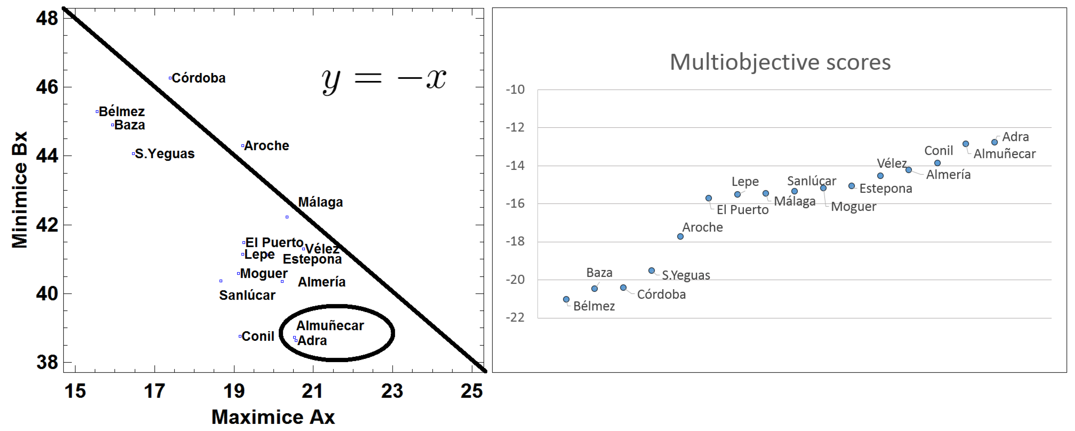
Figure A5. (left) Sites considering Ax and Bx and the function y = x . The places with high values of Ax (max) and low values of Bx (min) are the best locations for the solution of the multiobjective problem (round). (right) Multiobjective scores values obtained for each site projecting the point in the function y = x . High values of this score indicate better places to locate the tourism rural inn.
Mathematics 08 00085 g0a5
Figure A6. Distribution of the three areas described in Figure A4. A and B areas are in the coastline and C in the inner.
Mathematics 08 00085 g0a6
The solution of (A9) allow us to draw the sites with a 2 D plot considering the X axe as A x and the Y axe as B x . We observe that better places have high values of A x and low values of B x . Hence, we can sort the sites in order to achieve the objectives in a similar way as factorial analysis works (two factors, the maximum and the minimum, instead of m variables).

Appendix C. Algorithms

To solve the real problems posed in this work, the algorithms were developed in MATLAB. As pointed out in Section 5, our method relies on finding the generalized supporting vectors. Thus, we refer the reader to [8] (Appendix A.1) for the MATLAB code “sol_1.m” to compute a basis of generalized supporting vectors of a finite number of matrices A 1 , , A k , in other words, a solution of Problem (A10), which was originally posed and solved in [7]:
max i = 1 k A i x 2 2 x 2 = 1
The solution of the previous problem (see [7] (Theorem 3.3)) is given by
max x 2 = 1 i = 1 k A i x 2 2 = λ max i = 1 k A i T A i
and
arg max x 2 = 1 i = 1 k A i x 2 2 = V λ max i = 1 k A i T A i S 2 n
where λ max denotes the greatest eigenvalue and V denotes the associated eigenvector space. We refer the reader to [8] (Theorem 4.2) for a generalization of [7] (Theorem 3.3) to a infinite number of operators on an infinite dimensional Hilbert space.
As we pointed out in Theorem 8, the solution of the problem
max A x B x 1
exists if and only if ker ( B ) ker ( A ) . Here is a simple code to check this.
  •     function p=existence_sol(A,B)
  •     %%%%
  •     %%%% This function checks the existence of the solution of the
  •     %%%% problem
  •     %%%%
  •     %%%% max ||Ax||
  •     %%%% ||Bx||<=1
  •     %%%%
  •     %%%%%%%%%%%%%%%%%%%%%%%%%%%%%%%
  •     %%%%
  •     %%%% INPUT:
  •     %%%%
  •     %%%% A, B - the matrices involved in the problem
  •     %%%%
  •     %%%%%%%%%%%%%%%%%%%%%%%%%%%%%%%%
  •     %%%%
  •     %%%% OUTPUT:
  •     %%%%
  •     %%%% p - true if the problem has solution or false on the contrary
  •     %%%%
  •     %%%%%%%%%%%%%%%%%%%%%%%%%%%%%%%%
  •     KerB = null(B);
  •     dimKerB = size(KerB,2);
  •     KerA = null(A);
  •     dimKerA = size(KerA,2);
  •     if (dimKerB<=dimKerA) & (rank([KerB KerA])==dimKerA)
  •         p = true;
  •     else
  •         p = false;
  •     end
  • end
Now we present the code to solve the first case of the previous maxmin problem, that is, the case where ker ( B ) = { 0 } . We refer the reader to Section 5 on which this code is based.
  • function x = case_1(A, B)
  •     %%%%
  •     %%%% This function computes the solution of the problem
  •     %%%%
  •     %%%% max ||Ax||_2
  •     %%%% ||Bx||_2<=1
  •     %%%%
  •     %%%% in the case KerB={0}.
  •     %%%%%%%%%%%%%%%%%%%%%%%%%%%%%%%
  •     %%%%
  •     %%%% INPUT:
  •     %%%%
  •     %%%% A, B - the matrices involved in the problem
  •     %%%%
  •     %%%%%%%%%%%%%%%%%%%%%%%%%%%%%%%%
  •     %%%%
  •     %%%% OUTPUT:
  •     %%%%
  •     %%%% x - basis of unit  eigenvectors associated to lambda_max
  •     %%%%
  •     %%%%%%%%%%%%%%%%%%%%%%%%%%%%%%%%
  •     %%%%
  •     KerB = null(B);
  •     dimKerB = size(KerB,2);
  •     if (dimKerB ~= 0)
  •         display(’KerB~={0}’)
  •         x=[];
  •     else % KerB={0}
  •             M = A*pinv(B);              % M = A*B+
  •                                                      % B+ is the pseudoinverse matrix
  •             [lambda_max, y] = sol_1({M}); % where sol_1 is the algorithm in [5, Appendix A.1]
  •             [nrows_y ncols_y] = size(y);
  •             r_B = rank(B);
  •             counter = 0;
  •             for i=1:ncols_y
  •                 r = rank([B y(:,i)]);
  •                 if (abs(r_B - r)<1e-12)     % Here we check if rank(B) = rank ([B y0]).
  •                                 % A tolerance of 1e-12 is needed in
  •                                 % order to compare these two ranks.
  •                    counter = counter +1;
  •                    y0(:,counter) = y(:,i);
  •                 end
  •             end
  •             x = pinv(B)*y0;               % This is a basis of solutions of our problem
  • end
Next, we can compute the global solution of the maxmin problem by means of the following code. Again, we refer the reader to Section 5 on which this code is based.
  •     function x = sol_2(A, B)
  •     %%%%
  •     %%%% This function computes the solution of the problem
  •     %%%%
  •     %%%% max ||Ax||_2
  •     %%%% ||Bx||_2<=1
  •     %%%%
  •     %%%%%%%%%%%%%%%%%%%%%%%%%%%%%%%
  •     %%%%
  •     %%%% INPUT:
  •     %%%%
  •     %%%% A, B - the matrices involved in the problem
  •     %%%%
  •     %%%%%%%%%%%%%%%%%%%%%%%%%%%%%%%%
  •     %%%%
  •     %%%% OUTPUT:
  •     %%%%
  •     %%%% x - Supporting vector which is the solution of the problem
  •     %%%%
  •     %%%%%%%%%%%%%%%%%%%%%%%%%%%%%%%%
  •     %%%%
  •     p=existence_sol(A,B);
  •     if p==true
  •         n = size(B,2);
  •         KerB = null(B);
  •         dimKerB = size(KerB,2);
  •         if (dimKerB == 0)               % KerB = {0} This is the case 1
  •             x = case_1(A,B);             % x is the solution of our problem
  •         else % KerB~={0}
  •             [Br indices] = colsindep(B); %%% First we extract the
  •                                             %%% independent columns in B
  •             Ar = A(indices);        %%% We extract the same columns of A
  •                   %%% Now, Ker(Br)={0} so this is the case 1 treated above:
  •             xr = case_1(Ar,Br);
  •             [nrows_xr,ncols_xr] = size(xr);
  •             %%% Now we compute the matrix solutions x of the problem
  •             counter = 0;
  •             for j = 1:ncols_xr
  •                 for i=1:n
  •                     if ismember(i,indices)==1 %%% i is an index of the ones
  •                                           %%% defined above
  •                         counter = counter + 1;
  •                         x(i,j) = xr(counter,j);
  •                     else
  •                         x(i,j) = 0;
  •                     end
  •                 end
  •             end
  •         end
  •  
  •     else
  •         display(’This problem has no solution’);
  •         x=[];
  •     end
  • end
Notice that we use the case_1 function described above and a new function named colsindep.We include the code to implement this new function below.
  •     function [Dcolsind, indices]=colsindep(D)
  •     %%%%
  •     %%%% This function extracts r = rank(D) independent columns of the
  •     %%%% matrix D and the indices of the columns in D which are independent
  •     %%%%
  •     %%%%%%%%%%%%%%%%%%%%%%%%%%%%%%%
  •     %%%%
  •     %%%% INPUT:
  •     %%%%
  •     %%%% D - a matrix with rank r
  •     %%%%
  •     %%%%%%%%%%%%%%%%%%%%%%%%%%%%%%%%
  •     %%%%
  •     %%%% OUTPUT:
  •     %%%%
  •     %%%% Dcolsind - r independent columns in D
  •     %%%% indices - the indices of independent columns extracted from D
  •     %%%%%%%%%%%%%%%%%%%%%%%%%%%%%%%%
  •     r=rank(D);            %%% Compute the rank
  •     [Q R p]=qr(D,0);      %%% p is a permutation vector such that A(:,p)=Q*R
  •     indices=sort(p(1:r)); %%% The first r elements in p are the indices of the
  •                           %%% columns linearly independent in D
  •     Dcolsind=D(:,indices);%%% Extract these columns
  • end
The MATLAB code to compute the solution of the TMS coil problem (A6):
max E x 1 ψ 2 D ψ 2 1
with the matrix D : = E x 2 C , where C is the Cholesky matrix of L, and in this case it verifies that ker ( D ) = { 0 } . Recall that (A6) comes from (A1):
max E x 1 ψ 2 min E x 2 ψ 2 min ψ T L ψ
  • function psi = sol2_psi(Ex1, Ex2, L)
  •  
  •     C = chol(L);                    % Cholesky’s decomposition of matrix L = C’ * C
  •  
  •     A = Ex1;
  •     B = [Ex2;C];
  •  
  •     psi = case_1(A,B);           % We apply the algorithm to obtain the solutions
  • end
Finally, we provide the code to compute the solution of the optimal geolocation problem (A9):
max A x 2 D x 2 1
with matrix D : = B I 3 . Notice that it also verifies that ker ( D ) = { 0 } and A and B are composed by standardized variables. Recall that (A9) comes from (A7):
max A x 2 min B x 2 min x 2
  • function x = sol_2_geoloc(A, B)
  •  
  •     [rows,cols] = size(A);
  •     D = [B; eye(size(cols))];
  •  
  •     x = case_1(A,D);           % We apply the algorithm to obtain the solutions
  • end

References

  1. Huang, N.; Ma, C.F. Modified conjugate gradient method for obtaining the minimum-norm solution of the generalized coupled Sylvester-conjugate matrix equations. Appl. Math. Model. 2016, 40, 1260–1275. [Google Scholar] [CrossRef]
  2. Yassin, B.; Lahcen, A.; Zeriab, E.S.M. Hybrid optimization procedure applied to optimal location finding for piezoelectric actuators and sensors for active vibration control. Appl. Math. Model. 2018, 62, 701–716. [Google Scholar] [CrossRef]
  3. Bishop, E.; Phelps, R.R. A proof that every Banach space is subreflexive. Bull. Am. Math. Soc. 1961, 67, 97–98. [Google Scholar] [CrossRef] [Green Version]
  4. Bishop, E.; Phelps, R.R. The support functionals of a convex set. In Proceedings of Symposia in Pure Mathematics; American Mathematical Society: Providence, RI, USA, 1963; Volume VII, pp. 27–35. [Google Scholar]
  5. Lindenstrauss, J. On operators which attain their norm. Israel J. Math. 1963, 1, 139–148. [Google Scholar] [CrossRef]
  6. James, R.C. Characterizations of reflexivity. Stud. Math. 1964, 23, 205–216. [Google Scholar] [CrossRef] [Green Version]
  7. Cobos-Sánchez, C.; García-Pacheco, F.J.; Moreno-Pulido, S.; Sáez-Martínez, S. Supporting vectors of continuous linear operators. Ann. Funct. Anal. 2017, 8, 520–530. [Google Scholar] [CrossRef]
  8. Garcia-Pacheco, F.J.; Cobos-Sanchez, C.; Moreno-Pulido, S.; Sanchez-Alzola, A. Exact solutions to max∥x∥=1i=1Ti(x)∥2 with applications to Physics, Bioengineering and Statistics. Commun. Nonlinear Sci. Numer. Simul. 2020, 82, 105054. [Google Scholar] [CrossRef]
  9. García-Pacheco, F.J.; Naranjo-Guerra, E. Supporting vectors of continuous linear projections. Int. J. Funct. Anal. Oper. Theory Appl. 2017, 9, 85–95. [Google Scholar] [CrossRef]
  10. Cobos Sánchez, C.; Garcia-Pacheco, F.J.; Guerrero Rodriguez, J.M.; Hill, J.R. An inverse boundary element method computational framework for designing optimal TMS coils. Eng. Anal. Bound. Elem. 2018, 88, 156–169. [Google Scholar] [CrossRef]
  11. Bohnenblust, F. A characterization of complex Hilbert spaces. Portugal. Math. 1942, 3, 103–109. [Google Scholar]
  12. Kakutani, S. Some characterizations of Euclidean space. Jpn. J. Math. 1939, 16, 93–97. [Google Scholar] [CrossRef] [Green Version]
  13. Sánchez, C.C.; Rodriguez, J.M.G.; Olozábal, Á.Q.; Blanco-Navarro, D. Novel TMS coils designed using an inverse boundary element method. Phys. Med. Biol. 2016, 62, 73–90. [Google Scholar] [CrossRef]
  14. Marin, L.; Power, H.; Bowtell, R.W.; Cobos Sanchez, C.; Becker, A.A.; Glover, P.; Jones, A. Boundary element method for an inverse problem in magnetic resonance imaging gradient coils. Comput. Model. Eng. Sci. 2008, 23, 149–173. [Google Scholar]
  15. Marin, L.; Power, H.; Bowtell, R.W.; Cobos Sanchez, C.; Becker, A.A.; Glover, P.; Jones, I.A. Numerical solution of an inverse problem in magnetic resonance imaging using a regularized higher-order boundary element method. In Boundary Elements and Other Mesh Reduction Methods XXIX; WIT Press: Southampton, UK, 2007; Volume 44, pp. 323–332. [Google Scholar] [CrossRef] [Green Version]
  16. Wassermann, E.; Epstein, C.; Ziemann, U.; Walsh, V.; Paus, T.; Lisanby, S. Oxford Handbook of Transcranial Stimulation (Oxford Handbooks), 1st ed.; Oxford University Press: New York, NY, USA, 2008. [Google Scholar]
  17. Romei, V.; Murray, M.M.; Merabet, L.B.; Thut, G. Occipital Transcranial Magnetic Stimulation Has Opposing Effects on Visual and Auditory Stimulus Detection: Implications for Multisensory Interactions. J. Neurosci. 2007, 27, 11465–11472. [Google Scholar] [CrossRef]
  18. Koponen, L.M.; Nieminen, J.O.; Ilmoniemi, R.J. Minimum-energy Coils for Transcranial Magnetic Stimulation: Application to Focal Stimulation. Brain Stimul. 2015, 8, 124–134. [Google Scholar] [CrossRef] [Green Version]
  19. Koponen, L.M.; Nieminen, J.O.; Mutanen, T.P.; Stenroos, M.; Ilmoniemi, R.J. Coil optimisation for transcranial magnetic stimulation in realistic head geometry. Brain Stimul. 2017, 10, 795–805. [Google Scholar] [CrossRef] [Green Version]
  20. Gomez, L.J.; Goetz, S.M.; Peterchev, A.V. Design of transcranial magnetic stimulation coils with optimal trade-off between depth, focality, and energy. J. Neural Eng. 2018, 15, 046033. [Google Scholar] [CrossRef]
  21. Wang, B.; Shen, M.R.; Deng, Z.D.; Smith, J.E.; Tharayil, J.J.; Gurrey, C.J.; Gomez, L.J.; Peterchev, A.V. Redesigning existing transcranial magnetic stimulation coils to reduce energy: application to low field magnetic stimulation. J. Neural Eng. 2018, 15, 036022. [Google Scholar] [CrossRef]
  22. Grandy, W.T. Time Evolution in Macroscopic Systems. I. Equations of Motion. Found. Phys. 2004, 34, 1–20. [Google Scholar] [CrossRef] [Green Version]
  23. Sakurai, J.J. Modern Quantum Mechanics; Addison-Wesley Publishing Company: Reading, MA, USA, 1993. [Google Scholar]
  24. Sanchez, C.C.; Bowtell, R.W.; Power, H.; Glover, P.; Marin, L.; Becker, A.A.; Jones, A. Forward electric field calculation using BEM for time-varying magnetic field gradients and motion in strong static fields. Eng. Anal. Bound. Elem. 2009, 33, 1074–1088. [Google Scholar] [CrossRef]
  25. Jäntschi, L.; Bálint, D.; Bolboaca, S. Multiple Linear Regressions by Maximizing the Likelihood under Assumption of Generalized Gauss-Laplace Distribution of the Error. Comput. Math. Methods Med. 2016, 2016, 1–8. [Google Scholar] [CrossRef] [PubMed]
  26. Gil-García, I.C.; García-Cascales, M.S.; Fernández-Guillamón, A.; Molina-García, A. Categorization and Analysis of Relevant Factors for Optimal Locations in Onshore and Offshore Wind Power Plants: A Taxonomic Review. J. Mar. Sci. Eng. 2019, 7, 391. [Google Scholar] [CrossRef] [Green Version]
  27. Pérez Morales, A.; Castillo, F.; Pardo-Zaragoza, P. Vulnerability of Transport Networks to Multi-Scenario Flooding and Optimum Location of Emergency Management Centers. Water 2019, 11, 1197. [Google Scholar] [CrossRef] [Green Version]
  28. Choi, J.W.; Kim, M.K. Multi-Objective Optimization of Voltage-Stability Based on Congestion Management for Integrating Wind Power into the Electricity Market. Appl. Sci. 2017, 7, 573. [Google Scholar] [CrossRef] [Green Version]
  29. Zavala, G.R.; García-Nieto, J.; Nebro, A.J. Qom—A New Hydrologic Prediction Model Enhanced with Multi-Objective Optimization. Appl. Sci. 2019, 10, 251. [Google Scholar] [CrossRef] [Green Version]
  30. Susowake, Y.; Masrur, H.; Yabiku, T.; Senjyu, T.; Motin Howlader, A.; Abdel-Akher, M.; Hemeida, A.M. A Multi-Objective Optimization Approach towards a Proposed Smart Apartment with Demand-Response in Japan. Energies 2019, 13, 127. [Google Scholar] [CrossRef] [Green Version]
  31. ESTACIONES AGROCLIMÁTICAS. Available online: https://www.juntadeandalucia.es/agriculturaypesca/ifapa/ria/servlet/FrontController (accessed on 18 September 2019).