Quantitatively Inferring Three Mechanisms from the Spatiotemporal Patterns

Abstract

Although the diversity of spatial patterns has gained extensive attention on ecosystems, it is still a challenge to discern the underlying ecological processes and mechanisms. Dynamical system models, such partial differential equations (PDEs), are some of the most widely used frameworks to unravel the spatial pattern formation, and to explore the potential ecological processes and mechanisms. Here, comparing the similarity of patterned dynamics among Allen–Cahn (AC) model, Cahn–Hilliard (CH) model, and Cahn–Hilliard with population demographics (CHPD) model, we show that integrated spatiotemporal behaviors of the structure factors, the density-fluctuation scaling, the Lifshitz–Slyozov (LS) scaling, and the saturation status are useful indicators to infer the underlying ecological processes, even though they display the indistinguishable spatial patterns. First, there is a remarkable peak of structure factors of the CH model and CHPD model, but absent in AC model. Second, both CH and CHPD models reveal a hyperuniform behavior with scaling of −2.90 and −2.60, respectively, but AC model displays a random distribution with scaling of −1.91. Third, both AC and CH display uniform LS behaviors with slightly different scaling of 0.37 and 0.32, respectively, but CHPD model has scaling of 0.19 at short-time scales and saturation at long-time scales. In sum, we provide insights into the dynamical indicators/behaviors of spatial patterns, obtained from pure spatial data and spatiotemporal related data, and a potential application to infer ecological processes.

1. Introduction

The reaction–diffusion systems have been posed to address the spatially extended interactions among species or chemical substances since 1937 [1], when the traveling waves behaviors of the reaction–diffusion equations were discovered and studied. To date, the spatial systems are widely used to explore the spatiotemporal behaviors going beyond the initial frameworks such as existence and stability of spatial solutions in biology, geology, physics, and ecology [2,3,4,5,6,7,8,9]. The solutions to reaction–diffusion equations display diverse behaviors including the formation of traveling waves [10], wave-like phenomena [11], spatial self-organized patterns [12], and coarsening behaviors [13].

In mathematics, the spatial extend models can be classified into the following three categories with the simplest version. Firstly, the model describes the Brownian dispersion and growth-mortality processes on single species [14,15]. Herein, the species abundance can dynamically fluctuate around their equilibria that is limited by carrying capacity. Secondly, we can describe the mass-conserving systems with the Cahn–Hilliard model if species have a biased movement behavior such as a local density-dependent relationship [13,16,17,18]. In fact, both of these processes may exist in an ecological system that lead to a third theoretical model, the Cahn–Hilliard model with demographical processes of species [19,20,21]. These models display similar patterns for the reasonable parameters on the same systems. How to infer the underlying mechanisms from the spatial behaviors are crucial themes for ecologists. Many spatial hallmarks were proposed to characterize their spatiotemporal behaviors including spatial correlation functions [22,23], spatial structure factor [24], LS law [25,26,27], the exponent of cluster size [28], and the exponent of spatial fluctuations [29], but few studies are hitherto proposed to comprehensively compare the hallmarks on the above-mentioned models.

In this paper, we present a comprehensive comparison of three typical PDE systems in two-dimensional space: the Allen–Cahn model, the mass-conserving Cahn–Hilliard model, and the Cahn–Hilliard model with demographical processes. The central theme is the characterization of the spatiotemporal dynamics of such systems displaying a spatially patterned behavior. A key insight from our spatial analysis, provided in Section 4, is how spatial patterns and spatial fluctuations can be used to infer underlying ecological processes and mechanisms from the indicators of the spatial fluctuation, spatial structure factor, spatial correlation functions, and LS growth behavior. Importantly, different ecological processes may lead a similar spatial patterns in some systems even for strikingly different ecosystems. Here, our proposed integrated indicators have potential for distinguishing the underpinning patterned behaviors.

2. Theoretical Models

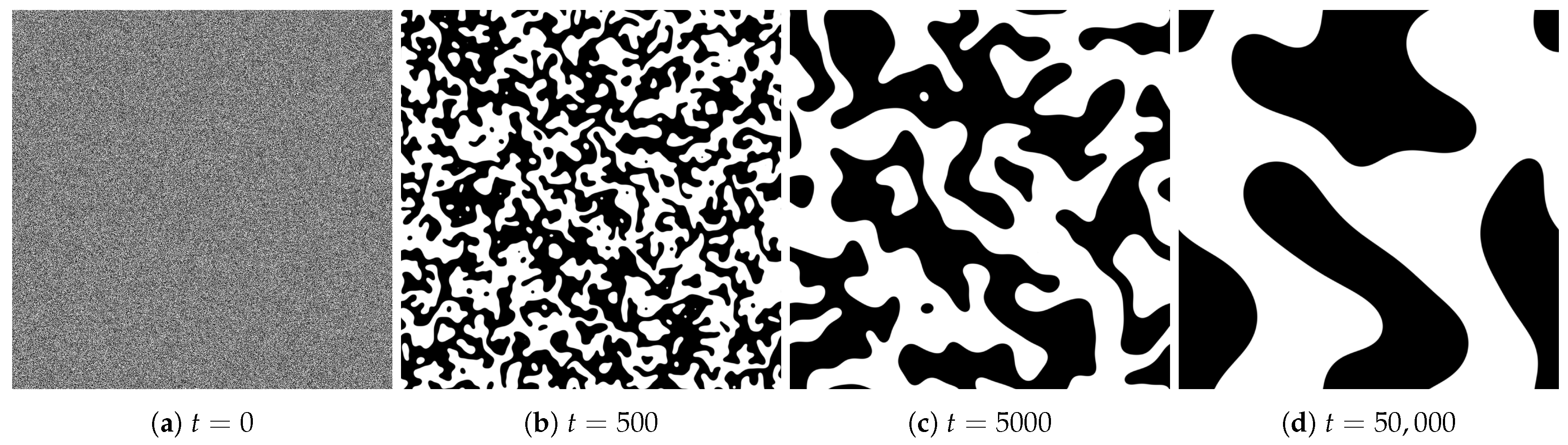
2.1. Allen–Cahn Model

The original Allen–Cahn model is a reaction–diffusion equation describing the phase separation process in a multi-component alloy system [30], including from disordered to ordered transitions. Recently, McNally et al. [18] showed that Allen–Cahn model can well describe the spatial pattern formation of microbial community, where microbes use T6SS to kill neighbors to separate the initially mixed flora, forming cloned plaques that grow over time. Theoretically, the model is given as follows assuming the species density as variable u at the time t within a spatial domain of $\mathsf{\Omega }$ ($\mathsf{\Omega }\subset R^2$), i.e.,

$$\begin{array}{cc}\hfill & u_t=-f\left(u\right)+\epsilon \mathsf{\Delta }u,u\in \mathsf{\Omega },\hfill \\ \hfill & \mathit{n}·\nabla u=0,u\in \partial \mathsf{\Omega },\hfill \end{array}$$

(1)

where $u_t$ is the partial derivative of u over time, $\epsilon$ is the diffusion coefficient, $\mathsf{\Delta }$ is the Laplacian operator, $\mathit{n}$ is the normal vector of the outer boundary, and ∇ is the gradient operator. Here, we take $f\left(u\right)=u(u-\alpha )(u-\beta )$, and $0<\alpha <\beta$, then the zero points of $f\left(u\right)$ is $u_0=0$, $\alpha$, and $\beta$. Here, $u_0$ are the equilibrium points of the model in Equation (1).

It can be easily proved that 0 and $\beta$ are stable equilibria of the model in Equation (1), whereas $\alpha$ is an unstable equilibrium. Over time, the solutions of the model in Equation (1) would be around 0 or $\beta$. In the spatial model in Equation (1), the solutions of phase separation will occur if $\epsilon >0$.

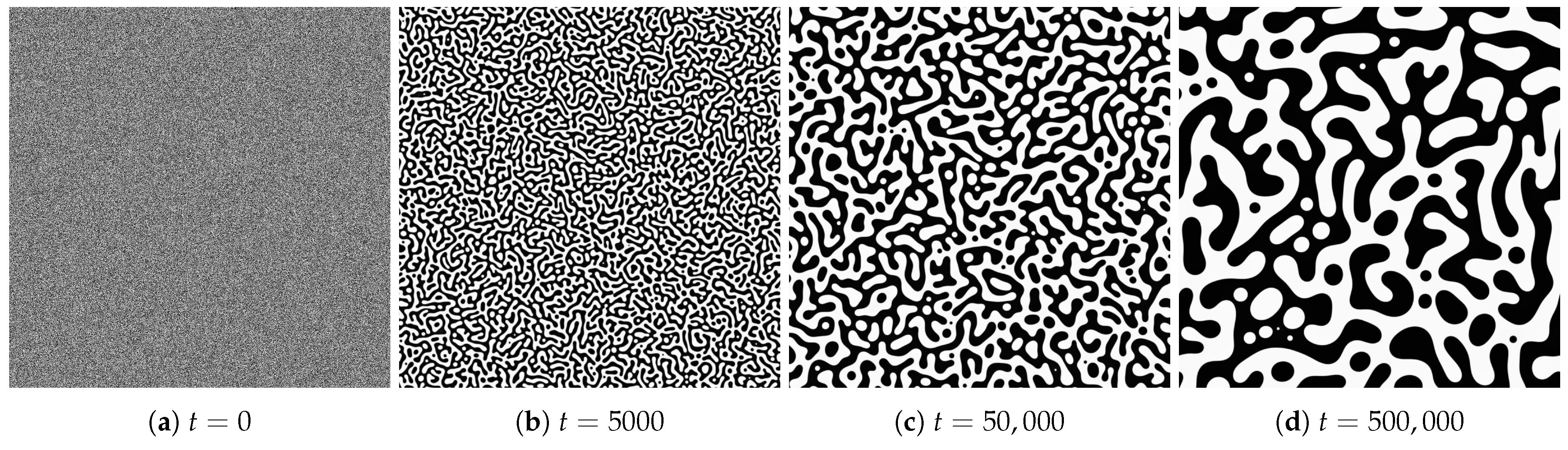
2.2. Cahn–Hilliard Model

The Cahn–Hilliard model describes the spontaneous separation of a mixed fluid into two pure phases [31], resulting in the formation of spatial patterns. This phase separation principle was used to elucidate the mechanism of pattern formation on small scales in a mussel bed ecosystem [13]. This self-organizing process results from the relationship between movement speed and local mussel density, which differs from the existing Turing principle. The general form of the Cahn–Hilliard model is given by

$$\begin{array}{cc}\hfill & u_t={\epsilon }_B\mathsf{\Delta }(f\left(u\right)-{\epsilon }_A\mathsf{\Delta }u),u\in \mathsf{\Omega },\hfill \\ \hfill & \mathit{n}·\nabla u=0,u\in \partial \mathsf{\Omega },\hfill \end{array}$$

(2)

where $u_t$ is the partial derivative of u over time, ${\epsilon }_A$ and ${\epsilon }_B$ are the local and nonlocal diffusion coefficients, $\mathsf{\Delta }$ is the Laplacian operator, $\mathit{n}$ is the normal vector of the outer boundary, and ∇ is the gradient operator. We take $f\left(u\right)=u(u-\alpha )(u-\beta )$ and $0<a<\beta$, then the zero points of $f\left(u\right)$ are $u_0=0$, $\alpha$, and $\beta$.

Mathematically, the stable equilibria of the Cahn–Hilliard model in Equation (2) are determined by the minimum values of the potential function $F\left(u\right)$ with $F^{\prime }\left(u\right)=f\left(u\right)$. Now, the potential function is expressed as $F\left(u\right)=\frac{1}{4}{u}^4-\frac{\alpha +\beta }{3}{u}^3+\frac{\alpha \beta }{2}{u}^2+C$ with constant C. $\alpha$ is the local maximum of $F\left(u\right)$, 0 and $\beta$ are the global minimum of $F\left(u\right)$. Therefore, 0 and $\beta$ are stable equilibria, and $\alpha$ is an unstable equilibrium. Note that Cahn–Hilliard model describes a mass-conservation ecosystem without mortality and birth processes.

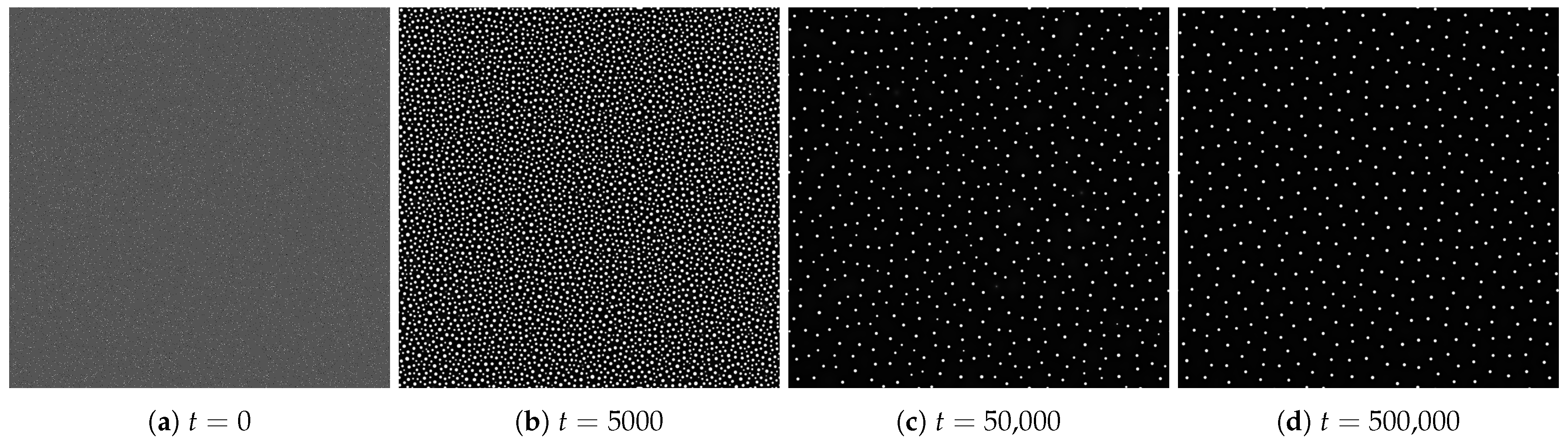
2.3. Cahn–Hilliard with Population Demographics Model

It is natural to ask that what will happen when the population demographics are involved in the Cahn–Hilliard model. In general, we address the Cahn–Hilliard model with a population demographics (hereafter, called CHPD), which describes the growth and aggregation of a single species [16]. A similar model was used to describe patterns formation result from density-dependent motility rather than traditional chemotaxis behavior [20]. The general model is given by

$$\begin{array}{cc}\hfill & u_t={\epsilon }_B\mathsf{\Delta }(f\left(u\right)-{\epsilon }_A\mathsf{\Delta }u)+ru(1-\frac{u}{K}),u\in \mathsf{\Omega },\hfill \\ \hfill & \mathit{n}·\nabla u=0,u\in \partial \mathsf{\Omega },\hfill \end{array}$$

(3)

where $u_t$ is the partial derivative of u over time, ${\epsilon }_A$ and ${\epsilon }_B$ are the local and nonlocal diffusion coefficients, and $\mathsf{\Delta }$ is the Laplacian operator. The last term is the logistic growth law, r $(r>0)$, is the net growth rate population, K is the environmental carrying capacity $(K>0)$, $\mathit{n}$ is the normal vector of the outer boundary, and ∇ is the gradient operator. Now, the equilibria of the model in Equation (3) are 0 and K.

Linearizing the nonspatial model in Equation (3) using a first-order Taylor expansion at $u_0=0$ and K, respectively, yields

$$u_t=g\left(u_0\right)+g^{\prime }\left(u_0\right)(u-u_0),$$

(4)

where $g^{\prime }\left(u\right)=r-\frac{2ur}{K}$. One sees that $u_0=0$ is an unstable equilibrium since $g^{\prime }\left(0\right)=r>0$, whereas $g^{\prime }\left(K\right)=-r<0$.

However, the spatial model in Equation (3) is linearized around $u\left(\mathbf{x}\right)=u_0$ in Fourier space, i.e., $u\left(\mathit{x}\right)=u_0+{\sum }_{\mathit{k}}{\delta }_{u_{\mathit{k}}}{e}^{i\mathit{k}·\mathit{x}+{\mathsf{\Lambda }}_{\mathit{k}}t}$ yields

$$\begin{array}{cc}\hfill & \dot{\delta }{u}_{\mathit{k}}={\mathsf{\Lambda }}_{\mathit{k}}{\delta }_{\mathit{k}},\hfill \\ \hfill & {\mathsf{\Lambda }}_{\mathit{k}}=-r-{\epsilon }_B{f}^{\prime }\left(u_0\right){\mathit{k}}^2-{\epsilon }_A{\epsilon }_B{\mathit{k}}^4,\hfill \end{array}$$

(5)

where $i=\sqrt{-1}$, $\mathit{x}$ is position, and $\mathit{k}$ is wave vector. If ${\mathsf{\Lambda }}_{\mathit{k}}\le 0$ is satisfied for all $\mathit{k}$, the system is stable. If ${\mathsf{\Lambda }}_{\mathit{k}}>0$ is established, the system is unstable. Since $r>0$, when $k=0$, ${\mathsf{\Lambda }}_{\mathit{k}}<0$. Hence, instability occurs if

$$\begin{array}{cc}\hfill & {\epsilon }_A{f}^{\prime }\left(u_0\right)<0,\hfill \\ \hfill & {\epsilon }_B{f}^{\prime }\left(u_0\right)f^{\prime }\left(u_0\right)>4{\epsilon }_{A}r.\hfill \end{array}$$

(6)

From this instability condition in Equation (6), one can see that the instability of the system is determined by the population growth rate (r) and the diffusion coefficients (${\epsilon }_A$ and ${\epsilon }_B$). If the logistic growth term is ignored, then 0 and $\beta$ are the stable equilibrium points and $\alpha$ is the unstable equilibrium point. The pattern of the model in Equation (3) will be phase separated at 0 and $\beta$. If both the diffusion term and the logistic term are considered, the phase separation is suppressed by the logistic growth term. Over time, the values of the patterned solution will be around 0 and K, which ascribes the Turing patterns.

3. Materials and Methods

3.1. Numerical Simulations

We use the finite difference methods [32] to solve the equation numerically in two dimensions. The Laplacian terms of the model in Equations (1)–(3) Care approximated by the following formula

$$\mathsf{\Delta }u(x,y)=\frac{u(x+\mathsf{\Delta }x,y)+u(x-\mathsf{\Delta }x,y)-2u(x,y)}{{\left(\mathsf{\Delta }x\right)}^2}+\frac{u(x,y+\mathsf{\Delta }y)+u(x,y-\mathsf{\Delta }y)-2u(x,y)}{{\left(\mathsf{\Delta }y\right)}^2},$$

(7)

with step length $\mathsf{\Delta }x=\frac{L_x}{m}=1.0$ and $\mathsf{\Delta }y=\frac{L_y}{m}=1.0$. Here, x and y indicate the spatial coordinate. $L_x$ and $L_y$ are the physical length of the simulation in x and y directions and m is the grid number. The numerical simulations were implemented in two-dimensional space with grid numbers from $L_x=L_y=2048$ to $L_x=L_y=\mathrm{20,000}$, and periodic boundary conditions. For AC and CH models, the initial values are random numbers with a mean of $0.5$. For CHPD model, the initial values are random numbers with a mean of $0.33$.

The iteration over time uses the first-order Euler method, i.e.,

$$u(x,y,t+\mathsf{\Delta }t)=u(x,y,t)+\mathsf{\Delta }tf\left(u\right),$$

(8)

with $\mathsf{\Delta }t=0.0025$ that satisfied the stability condition [33].

All numerical simulations were implemented in Python 3.7 (Python Software Foundation, CWI, Amsterdam, Netherlands) and MATLAB 2019a (The MathWorks Inc., Natick, MA, USA). PyOpencl (https://documen.tician.de/pyopencl/) was used to accelerate the simulations; the code is available from Github (https://github.com/Kang-Zhang).

3.2. Spatial Correlation Functions

Spatial correlation function is widely applied to characterized spatial structure and its correlations biophysics [34]. It is usually expressed as

$$\begin{array}{c}\hfill g({\mathit{r}}_i,{\mathit{r}}_j)=\langle (\phi \left({\mathit{r}}_i\right)-\langle \phi \left({\mathit{r}}_j\right)\rangle )\times (\phi \left({\mathit{r}}_j\right)-\langle \phi \left({\mathit{r}}_j\right)\rangle )\rangle =\langle \phi \left({\mathit{r}}_i\right)\phi \left({\mathit{r}}_j\right)\rangle -\langle \phi \left({\mathit{r}}_i\right)\rangle \langle \phi \left({\mathit{r}}_j\right)\rangle ,\end{array}$$

(9)

where ${\mathit{r}}_i$ and ${\mathit{r}}_j$ are two different locations; $\phi \left({\mathit{r}}_i\right)$, $\phi \left({\mathit{r}}_i\right)$ are numerical solutions at ${\mathit{r}}_i$ and ${\mathit{r}}_j$, respectively; and $\langle \rangle$ is the mathematical expectation. Thus, $g({\mathit{r}}_i,{\mathit{r}}_j)$ depends only on the displacement $\mathit{r}$ between the two locations. That is,

$$g({\mathit{r}}_i,{\mathit{r}}_j)=g({\mathit{r}}_i,{\mathit{r}}_i+\mathit{r})=g\left(\mathit{r}\right).$$

(10)

Thus, the average of the correlation functions of all two points with a displacement of $\mathit{r}$ is obtained as follows

$$g\left(r\right)=\langle \sum _{\mid {\mathit{r}}_i-{\mathit{r}}_j\mid =r}[\langle \phi \left({\mathit{r}}_i\right)\phi \left({\mathit{r}}_j\right)\rangle -\langle \phi \left({\mathit{r}}_i\right)\rangle \langle \phi \left({\mathit{r}}_j\right)\rangle ]\rangle .$$

(11)

The spatial correlation function is a measure of the correlation of a variable between two spatial positions. If the value of the variable fluctuates in one direction at the same time, a positive value is taken; otherwise, a negative value is taken. If their fluctuations are completely unrelated, then the value is zero.

3.3. Structure Factors

Structure factor is an important indicator for analyzing long-range spatial correlations and scattering that is a function of scattering vector ($\mathit{k}$) and time (t). The normalized structural factor [35] is written as

$$s(\mathit{k},t)=\frac{\langle \frac{1}{N}|{\sum }_r{exp}^{-i\mathit{k}·\mathit{r}}[\phi (\mathit{r},t)-\langle \phi \rangle ]{|}^2\rangle }{\langle {\phi }^2\left(t\right)\rangle -{\langle \phi \rangle }^2},$$

(12)

where $\phi (\mathit{r},t)$ is the numerical solution at time t and position $\mathit{r}$ and $\langle \phi \rangle$ is the mean of all $\phi (\mathit{r},t)$. Here, the structural factors $s(\mathit{k},t)$ are obtained by the Fourier transform on the solutions, and then the square of the modulus is taken and averaged in all directions.

3.4. Density Fluctuation

Density fluctuation is a measure to directly quantify observations of local crowd density, the rules that predict mass behaviors under new circumstances [36,37]. In a spherical window of radius R, the local variance ${\sigma }_{\phi }^2\left(R\right)$ associated with field fluctuations can be expressed in terms of the autocovariance function or the spectral function [29]. It is given by

$$\begin{array}{c}\hfill {\sigma }_{\phi }^2\left(R\right)=\frac{1}{v_1\left(R\right)}{\int }_{R^d}\psi \left(\mathit{r}\right){\alpha }_2(\mathit{r};R)d\mathit{r}=\frac{1}{v_1\left(R\right){\left(2\pi \right)}^d}{\int }_{R^d}\tilde{\psi }\left(\mathit{k}\right){\tilde{\alpha }}_2(\mathit{k};R)d\mathit{k},\end{array}$$

(13)

where $v_1\left(R\right)$ is the volume of a d-dimensional sphere of radius R; $\mathit{r}={\mathit{r}}_2-{\mathit{r}}_1$. $\psi \left(\mathit{r}\right)$ describes the autocorrelation functions, i.e., $\langle (\phi \left({\mathit{r}}_1\right)-\langle \phi \left({\mathit{r}}_1\right)\rangle )(\phi \left({\mathit{r}}_2\right)-\langle \phi \left({\mathit{r}}_2\right)\rangle )\rangle$; and $\tilde{\psi }\left(\mathit{k}\right)$ depicts the Fourier transform of $\psi \left(\mathit{r}\right)$. ${\alpha }_2(\mathit{r};R)$ is the scaled intersection volume [37] of two spherical windows with radius r and R and ${\tilde{\alpha }}_2(\mathit{k};R)$ is its Fourier transform. One can call that $\phi$ is a hyperuniform state if its autocorrelation function subjects to the condition

$${\int }_{R^d}\psi \left(\mathit{r}\right)d\mathit{r}=0.$$

(14)

4. Results and Discussion

4.1. Spatial Patterns

Allen–Cahn model reveals a continual coarsening behavior, where cluster size become bigger and bigger and converge to one of its stable states, as shown in Figure 1. The system only displays a characteristic spatial scale at certain stages. A scale-free behavior appears at early stages. On the contrary, Cahn–Hilliard model displays a clearly characteristic spatial scale (Figure 2), and this scale follows a power law relationship with time. They are indistinguishable spatial patterns from Turing patterns (cf. Figure 2 and Figure 3). It is notable that CH model describes the mass-conservation ecological processes that remarkably differ from the Allen–Cahn model despite both models reveal a coarsening behavior. The CHPD model displays classical Turing patterns with a stationary spatial scale when we consider a species birth–mortality process (Figure 3). In sum, it is difficult to infer the underlying ecological processes and potential mechanism from the merely observed spatial patterns.

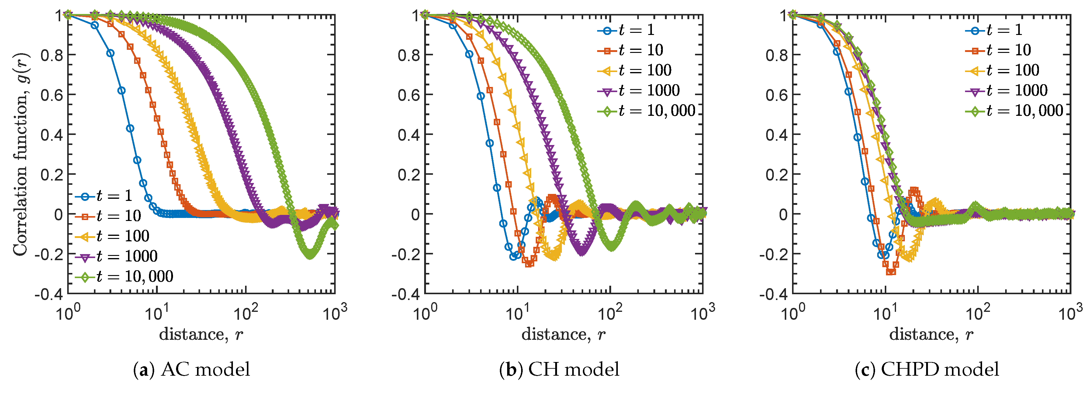
4.2. Spatial Correlation Functions

Figure 4 illustrates the spatial correlation of the three models from $t=1$ to $t=$ 10,000. The spatial correlation functions reveal differently dampened oscillation behaviors at long time scales, where the location of minimal values increases with time (Figure 4). It is consistent with the coarsening processes of the spatial patterns. However, this behavior is not obvious in AC model, which means that the pattern has no characteristic scale. In sum, the spatial correlation function is not a significant indicator to distinguish three models.

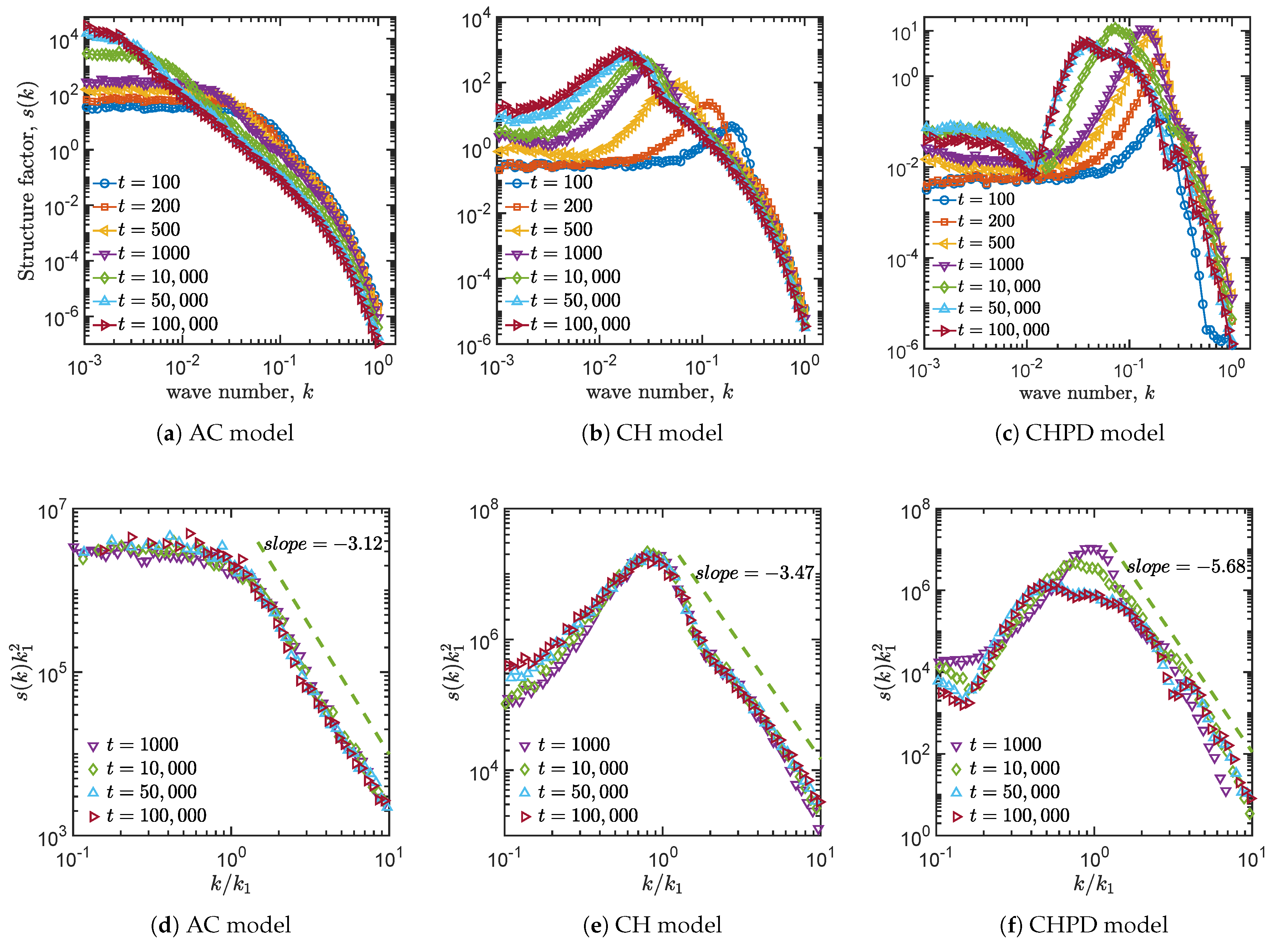
4.3. Structure Factors

To investigate the characteristic wavelength of the patterns, we plot the structural factor $s(\mathit{k},t)$ versus wave numbers $\mathit{k}$ at different times in Figure 5. A larger value of $s(\mathit{k},t)$ means a stronger dominant effect of its wave numbers.

For AC model, there is no dominant wave numbers of $s\left(\mathit{k}\right)$, implying absence of spatial characteristic length on this system. It displays a power law decline with exponent of −3.12, predicting scale-free patterns (Figure 5d). However, $s\left(\mathit{k}\right)$ has obvious dominant peak in the CH and CHPD models, indicating the regular spatial patterns. Furthermore, with time, the peak shifts to a smaller wave number, indicating that the spatial characteristic length is gradually increasing. For CHPD model, there is no significant change in the structure factor after a critical time scale (here 50,000), indicating that the spatial patterns do not change over time. This saturated behavior indicates the logistic growth term is playing a leading role (the phase separation is suppressed). In sum, the structure factors can serve as an excellent indicator to distinguish AC and CH/CHPD model.

Moreover, all systems display a universal scaling behavior at high wave numbers (i.e., small wavelength). They collapse to master curves when the structure factors were normalized by $k/k_1$ for different times [38], as shown in Figure 5d–f. Unfortunately, to date we do not know the ecological significance of those slope values.

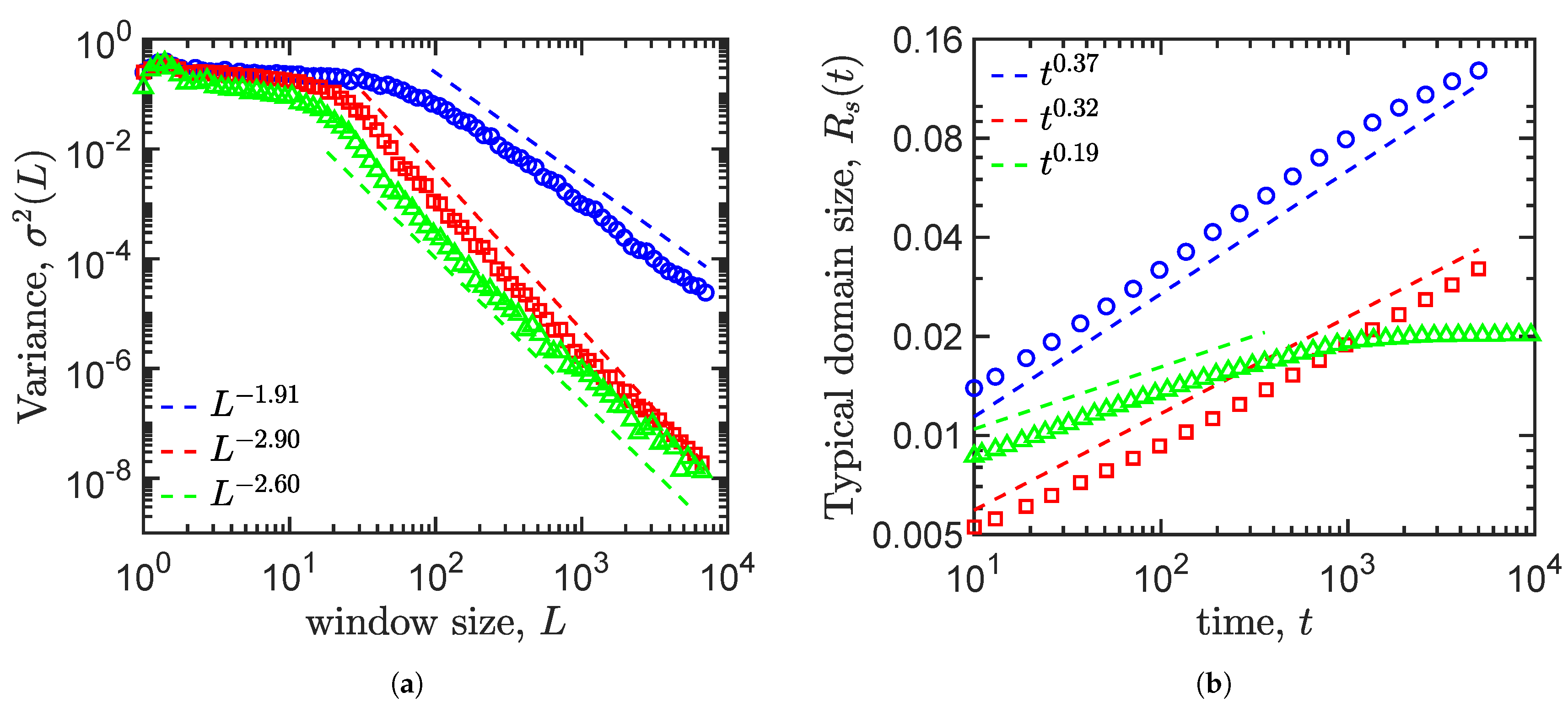
4.4. Density Fluctuation

The exponent of density fluctuation can be used to quantitatively measure the spatial distribution of the pattern [36,37]. As mentioned in the Method Section, we plot the variable-field fluctuations as a function of the window size L in Figure 6a. As expected, the exponent of density fluctuations predicts remarkable differences between AC model and CH/CHPD model despite it being impossible to directly distinguish from spatial patterns (cf. Figure 1, Figure 2 and Figure 3). The exponent of the AC model is around −1.91, implying a random distribution of patterns at large-spatial scales. Interestingly, CH and CHPD models have the exponents of −2.90 and −2.60, respectively. Generally, this exponential value of the scaling law is used to describe the spatial-ordered features. It is called “hyperuniformity” when the exponent of the density fluctuation is less than −2.0, where the long-wavelength density fluctuations are suppressed [39]. In sum, the exponent of density fluctuation is also useful to quantify the spatial patterns between AC model and CH/CHPD models.

4.5. Growth Law

To measure how the spatial structure of the patterns evolves over time, we calculate the characteristic length, $R_s\left(t\right)$, with location of the maximum of $s(\mathit{k},t)$ and its first moment at time t, i.e.,

$$k_1\left(t\right)=\frac{{\sum }_{k}ks(\mathit{k},t)}{{\sum }_{k}s(\mathit{k},t)}.$$

(15)

Then, the spatial characteristic length (also called wavelength) change over time can be obtained as

$$R_s\left(t\right)=\frac{2\pi }{k_1\left(t\right)}.$$

(16)

The scaling behaviors of the spatial wavelength $R_s\left(t\right)$ are shown in Figure 6b. The AC and CH models reveal power law relationship with exponents around 0.37 and 0.32, respectively. It should be noted that this scaling property is called the Lifshitz–Slyozov–Wagner law [40]. However, CHPD model has phase separation patterns at an early stage with scaling of 0.19, but it saturates at long-time scales. These patterns are equivalent to the Turing principle. In sum, this saturated behavior of growth rate can well distinguish CH model and CHPD model, which are impossible to be separated by structure factor, density fluctuation, and spatial correlation function (see

Table 1. Summary of the different indicators on three mechanism models.

Model Types	Structure Factors	Density Fluctuation	Growth Law	Saturation
Allen–Cahn	−3.12	−1.91	0.37	No
Cahn–Hillard	−3.47	−2.90	0.32	No
Cahn–Hillard and logistic term	−5.68	−2.60	0.19	Yes
Validity of the indicators	Yes	Yes	Yes	Yes

for summary).

5. Conclusions

Although PDE models have been widely used to describe the spatial patterns in many ecological and biological systems, few studies focus on inferring the linkage between these visual patterned characters and their potential mechanisms [41,42,43]. To do this, one of the effective ways is to build the quantitative indicators of these macrocosm patterns, which can serve as the hallmarks of the underlying ecological processes. Thus, it is a key issue to explain the ecological mechanisms by comparing the temporal and spatial behavior of the spatial patterns [44,45,46].

Here, we use structure factors, density fluctuation, growth law, and saturation status (Table 1) to quantify the spatiotemporal dynamics of AC model, CH model, and CHPD model. There is a remarkable peak of structure factors in the CH model and CHPD model, but absent in AC model. The differences of spatial structures between the AC model and CH/CHPD model can be well distinguished by the exponent of density fluctuations. Both CH and CHPD models reveal a hyperuniform behavior with scaling of −2.90 and −2.60, respectively, but AC model displays a random distribution with scaling of −1.91. The differences in time scales among the patterns of the three models can be well distinguished by LS behaviors. Both AC and CH model display the LS behaviors with scaling of 0.37 and 0.32, respectively, but CHPD model with scaling of 0.19 at short-time scales and saturation at long-time scales.

We showed that the underlying mechanisms can well be identified by the spatial information, i.e., the structure factors, the density fluctuation, the growth law, and the saturation; however, seeking real ecological cases is still a challenge (see

Table 2. A summary of the three mechanisms on spatial self-organization in ecosystems.

Model	Ecosystem	Ecological Processes	Refs.
AC	Bacteria (Vibrio cholerae)	Phase separation caused by competition	[18]
	Plant (Centaurea maculosa)	Allelopathy and exotic plant invasion	[50]
	Coral reef	Allelopathy and spatial competition	[51]
CH	Mussels	Density-dependent movement behavior	[8,13]
	Ants	Density-dependent movement behavior	[52]
	Bacteria (Escherichia coli)	Density-dependent chemo-taxis behavior	[53,54]
	Birds	Resource-dependent movement behavior	[55]
	Elk (Cervus canadensis)	Socially inform	[56]
	Zebrafish	Run-and-chase behavior movement	[57]
	Sperm	Integrated geometry with minima drag	[58]
CHPD	Bacteria (Escherichia coli, Bacillus subtilis)	Density-dependent motility and birth-death	[19,20]
	Stones and soil	Freeze–thaw cycles	[59]
	Insect	General theory	[16]

for summary). To the best of our knowledge, the first indicator (structure factors) can be applied to calculate the spatial wavelength, with only spatial data. The second indicator (density fluctuation) can distinguish the random distribution and the hyperuniform state at large spatial scales. It also reveals the intensity of long wave suppression. The third indicator (growth law) can be obtained from the spatiotemporal observed sequences. It describes the change and the stability of spatial structure with time. There are still many other potential mechanisms to generate spatially self-organized patterns in the ecosystems [47,48] such as animal aggregation due to taxis and density-dependence [49], but they are beyond the scope of the discussion here. It is interesting for further comparison in the future research.

To sum, we find that the density-fluctuation exponent and LS behaviors can quantitatively infer the three underlying mechanisms from the spatiotemporal patterns. We need to integrate multiple indicators to distinguish the underlying ecological processes and mechanisms, such as Turing principle and phase separation principle.

References

1. Fisher, R.A. The wave of advance of advntageous genes. Ann. Eugen. 1937, 7, 355–369. [Google Scholar] [CrossRef] [Green Version]
2. Murray, J.D. Mathematical Biology; Springer: Berlin, Germany, 2002. [Google Scholar]
3. Woodward, D.E.; Tyson, R.; Myerscough, M.R.; Murray, J.D.; Budrene, E.O.; Berg, H.C. Spatio-temporal patterns generated by Salmonella typhimurium. Biophys. J. 1995, 68, 2181–2189. [Google Scholar] [CrossRef] [Green Version]
4. Meinhardt, H. The Algorithmic Beauty of Sea Shells; Springer Science & Business Media: Berlin/Heidelberg Germany, 2009. [Google Scholar]
5. Klausmeier, C.A. Regular and irregular patterns in semiarid vegetation. Science 1999, 284, 1826–1828. [Google Scholar] [CrossRef]
6. Ouyang, Q.; Swinney, H.L. Transition from a Uniform State to Hexagonal and Striped Turing Patterns. Nature 1991, 352, 610–612. [Google Scholar] [CrossRef]
7. Kondo, S.; Miura, T. Reaction-Diffusion Model as a Framework for Understanding Biological Pattern Formation. Science 2010, 329, 1616–1620. [Google Scholar] [CrossRef] [Green Version]
8. Van de Koppel, J.; Rietkerk, M.; Dankers, N.; Herman, P.M.J. Scale-Dependent Feedback and Regular Spatial Patterns in Young Mussel Beds. Am. Nat. 2005, 165, 66–77. [Google Scholar] [CrossRef] [Green Version]
9. Segel, L.A.; Jackson, J.L. Dissipative structure: An explanation and an ecological example. J. Theor. Biol. 1972, 37, 545–559. [Google Scholar] [CrossRef]
10. Cabrera, C.V. Lateral inhibition and cell fate during neurogenesis in Drosophila: The interactions between scute, Notch and Delta. Development 1990, 110, 733–742. [Google Scholar]
11. Dormann, D.; Weijer, C.J. Propagating chemoattractant waves coordinate periodic cell movement in Dictyostelium slugs. Development 2001, 128, 4535–4543. [Google Scholar]
12. Rietkerk, M.; van de Koppel, J. Regular pattern formation in real ecosystems. Trends Ecol. Evol. 2008, 23, 169–175. [Google Scholar] [CrossRef]
13. Liu, Q.X.; Doelman, A.; Rottschäfer, V.; de Jager, M.; Herman, P.M.; Rietkerk, M.; van de Koppel, J. Phase separation explains a new class of self-organized spatial patterns in ecological systems. Proc. Natl. Acad. Sci. USA 2013, 110, 11905–11910. [Google Scholar] [CrossRef] [Green Version]
14. Aihara, S.; Takaki, T.; Takada, N. Multi-phase-field modeling using a conservative Allen–Cahn equation for multiphase flow. Comput. Fluids 2019, 178, 141–151. [Google Scholar] [CrossRef]
15. Allen, S.M.; Cahn, J.W. Ground state structures in ordered binary alloys with second neighbor interactions. Acta Metall. 1972, 20, 423–433. [Google Scholar] [CrossRef]
16. Cohen, D.S.; Murray, J.D. A Generalized Diffusion-Model for Growth and Dispersal in a Population. J. Math. Biol. 1981, 12, 237–249. [Google Scholar] [CrossRef]
17. Liu, Q.X.; Rietkerk, M.; Herman, P.M.; Piersma, T.; Fryxell, J.M.; van de Koppel, J. Phase separation driven by density-dependent movement: A novel mechanism for ecological patterns. Phys. Life Rev. 2016, 19, 107–121. [Google Scholar] [CrossRef] [Green Version]
18. McNally, L.; Bernardy, E.; Thomas, J.; Kalziqi, A.; Pentz, J.; Brown, S.P.; Hammer, B.K.; Yunker, P.J.; Ratcliff, W.C. Killing by Type VI secretion drives genetic phase separation and correlates with increased cooperation. Nat. Commun. 2017, 8, 14371. [Google Scholar] [CrossRef]
19. Vicsek, T. Ecological patterns emerging as a result of the density distribution of organisms: Comment on “Phase separation driven by density-dependent movement: A novel mechanism for ecological patterns” by Quan-Xing Liu et al. Phys. Life Rev. 2016, 19, 139–141. [Google Scholar] [CrossRef]
20. Cates, M.E.; Marenduzzo, D.; Pagonabarraga, I.; Tailleur, J. Arrested phase separation in reproducing bacteria creates a generic route to pattern formation. Proc. Natl. Acad. Sci. USA 2010, 107, 11715–11720. [Google Scholar] [CrossRef] [Green Version]
21. Wittkowski, R.; Tiribocchi, A.; Stenhammar, J.; Allen, R.J.; Marenduzzo, D.; Cates, M.E. Scalar ϕ4 field theory for active-particle phase separation. Nat. Commun. 2014, 5, 4351. [Google Scholar] [CrossRef] [Green Version]
22. Toral, R.; Chakrabarti, A.; Gunton, J.D. Droplet distribution for the two-dimensional Cahn-Hilliard model: Comparison of theory with large-scale simulations. Phys. Rev. A 1992, 45, 2147–2150. [Google Scholar] [CrossRef]
23. Chen, X.; Dong, X.; Be’er, A.; Swinney, H.L.; Zhang, H.P. Scale-Invariant Correlations in Dynamic Bacterial Clusters. Phys. Rev. Lett. 2012, 108, 148101. [Google Scholar] [CrossRef]
24. Zhu, J.; Chen, L.-Q.; Shen, J.; Tikare, V. Coarsening kinetics from a variable-mobility Cahn-Hilliard equation: Application of a semi-implicit Fourier spectral method. Phys. Rev. E 1999, 60, 3564–3572. [Google Scholar] [CrossRef] [Green Version]
25. Collet, J.F.; Goudon, T. On solutions of the Lifshitz-Slyozov model. Nonlinearity 2000, 13, 1239–1262. [Google Scholar] [CrossRef]
26. Kukushkin, S.A.; Slyozov, V.V. Theory of the Ostwald ripening in multicomponent systems under non-isothermal conditions. J. Phys. Chem. Solids 1996, 57, 195–204. [Google Scholar] [CrossRef]
27. Svoboda, J.; Fischer, F.D. Generalization of the Lifshitz-Slyozov-Wagner coarsening theory to non-dilute multi-component systems. Acta Mater 2014, 79, 304–314. [Google Scholar] [CrossRef]
28. Kéfi, S.; Rietkerk, M.; Alados, C.L.; Pueyo, Y.; Papanastasis, V.P.; ElAich, A.; De Ruiter, P.C. Spatial vegetation patterns and imminent desertification in Mediterranean arid ecosystems. Nature 2007, 449, 213–215. [Google Scholar] [CrossRef]
29. Torquato, S. Hyperuniform states of matter. Phys. Rep. 2018, 745, 1–95. [Google Scholar] [CrossRef] [Green Version]
30. Allen, S.M.; Cahn, J.W. A microscopic theory for antiphase boundary motion and its application to antiphase domain coarsening. Acta Metall. 1979, 27, 1085–1095. [Google Scholar] [CrossRef]
31. Cahn, J.W.; Hilliard, J.E. Free energy of a nonuniform system. I. Interfacial free energy. J. Chem. Phys. 1958, 28, 258–267. [Google Scholar] [CrossRef]
32. Chow, S.-N.; Conti, R.; Johnson, R.; Mallet-Paret, J.; Nussbaum, R. Dynamical systems: Lectures Given at the CIME Summer School Held in Cetraro, Italy, June 19–26, 2000; Springer: Berlin, Germany, 2003. [Google Scholar]
33. Richtmyer, R.D.; Dill, E. Difference methods for initial-value problems. Phys. Today 1959, 12, 50. [Google Scholar] [CrossRef]
34. Newman, M.; Barkema, G. Monte Carlo Methods in Statistical Physics; Oxford University Press: New York, NY, USA, 1999. [Google Scholar]
35. Toral, R.; Chakrabarti, A.; Gunton, J.D. Large scale simulations of the two-dimensional Cahn-Hilliard model. Phys. A Stat. Mech. Its Appl. 1995, 213, 41–49. [Google Scholar] [CrossRef]
36. Zhang, H.P.; Be’er, A.; Florin, E.L.; Swinney, H.L. Collective motion and density fluctuations in bacterial colonies. Proc. Natl. Acad. Sci. USA 2010, 107, 13626–13630. [Google Scholar] [CrossRef] [PubMed] [Green Version]
37. Klatt, A.M.; Torquato, S. Characterization of maximally random jammed sphere packings. II. Correlation functions and density fluctuations. Phys. Rev. E 2016, 94, 022152. [Google Scholar] [CrossRef] [Green Version]
38. Brown, G.; Rikvold, P.A.; Grant, M. Universality and scaling for the structure factor in dynamic order-disorder transitions. Phys. Rev. E 1998, 58, 5501–5507. [Google Scholar] [CrossRef] [Green Version]
39. Lei, Q.L.; Ni, R. Hydrodynamics of random-organizing hyperuniform fluids. Proc. Natl. Acad. Sci. USA 2019, 116, 22983–22989. [Google Scholar] [CrossRef] [Green Version]
40. Cheng, S.Z. Phase Transitions in Polymers: The Role of Metastable States; Elsevier: Amsterdam, The Netherlands, 2008. [Google Scholar]
41. Hammond, M.P.; Kolasa, J. Spatial variation as a tool for inferring temporal variation and diagnosing types of mechanisms in ecosystems. PLoS ONE 2014, 9, e89245. [Google Scholar] [CrossRef]
42. Borgogno, F.; D’Odorico, P.; Laio, F.; Ridolfi, L. Mathematical models of vegetation pattern formation in ecohydrology. Rev. Geophys. 2009, 47. [Google Scholar] [CrossRef]
43. Liu, Q.X.; Weerman, E.J.; Herman, P.M.; Olff, H.; van de Koppel, J. Alternative mechanisms alter the emergent properties of self-organization in mussel beds. Proc. R. Soc. B Biol. Sci. 2012, 279, 2744–2753. [Google Scholar] [CrossRef] [Green Version]
44. Ball, P. Patterns in Nature: Why the Natural World Looks the Way it Does; University of Chicago Press: Chicago, IL, USA, 2006. [Google Scholar]
45. Mueller, E.N.; Wainwright, J.; Parsons, A.J.; Turnbull, L. Patterns of Land Degradation in Drylands; Springer: Berlin, Germany, 2014. [Google Scholar]
46. Thompson, S.E.; Daniels, K.E. A Porous Convection Model for Grass Patterns. Am. Nat. 2010, 175, 10–15. [Google Scholar] [CrossRef]
47. Petrovskii, S. Pattern, process, scale, and model’s sensitivity Comment on “Phase separation driven by density-dependent movement: Anovel mechanism for ecological patterns”. Phys. Life Rev. 2016, 19, 131–134. [Google Scholar] [CrossRef]
48. Ellis, J.; Petrovskaya, N.; Petrovskii, S. Effect of density-dependent individual movement on emerging spatial population distribution: Brownian motion vs Levy flights. J. Theor. Biol. 2019, 464, 159–178. [Google Scholar] [CrossRef] [Green Version]
49. Tyutyunov, Y.; Senina, I.; Arditi, R. Clustering due to acceleration in the response to population gradient: A simple self-organization model. Am. Nat. 2004, 164, 722–735. [Google Scholar] [CrossRef]
50. Bais, H.P.; Vepachedu, R.; Gilroy, S.; Callaway, R.M.; Vivanco, J.M. Allelopathy and exotic plant invasion: From molecules and genes to species interactions. Science 2003, 301, 1377–1380. [Google Scholar] [CrossRef]
51. Jackson, J.B.C.; Buss, L.E.O. Alleopathy and spatial competition among coral reef invertebrates. Proc. Natl. Acad. Sci. USA 1975, 72, 5160–5163. [Google Scholar] [CrossRef] [Green Version]
52. Theraulaz, G.; Bonabeau, E.; Nicolis, S.C.; Solé, R.V.; Fourcassié, V.; Blanco, S.; Fournier, R.; Joly, J.L.; Fernández, P.; Grimal, A.; et al. Spatial patterns in ant colonies. Proc. Natl. Acad. Sci. USA 2002, 99, 9645–9649. [Google Scholar] [CrossRef] [Green Version]
53. Liu, C.; Fu, X.; Liu, L.; Ren, X.; Chau, C.K.; Li, S.; Xiang, L.; Zeng, H.; Chen, G.; Tang, L.H.; et al. Sequential establishment of stripe patterns in an expanding cell population. Science 2011, 334, 238–241. [Google Scholar] [CrossRef] [Green Version]
54. Fu, X.; Tang, L.H.; Liu, C.; Huang, J.D.; Hwa, T.; Lenz, P. Stripe formation in bacterial systems with density-suppressed motility. Phys. Rev. Lett. 2012, 108, 198102. [Google Scholar] [CrossRef] [Green Version]
55. Folmer, E.O.; Olff, H.; Piersma, T. The spatial distribution of flocking foragers: Disentangling the effects of food availability, interference and conspecific attraction by means of spatial autoregressive modeling. Oikos 2012, 121, 551–561. [Google Scholar] [CrossRef] [Green Version]
56. Haydon, D.T.; Morales, J.M.; Yott, A.; Jenkins, D.A.; Rosatte, R.; Fryxell, J.M. Socially informed random walks: Incorporating group dynamics into models of population spread and growth. Proc. R. Soc. B Biol. Sci. 2008, 275, 1101–1109. [Google Scholar] [CrossRef] [Green Version]
57. Yamanaka, H.; Kondo, S. In vitro analysis suggests that difference in cell movement during direct interaction can generate various pigment patterns in vivo. Proc. Natl. Acad. Sci. USA 2014, 111, 1867–1872. [Google Scholar] [CrossRef] [Green Version]
58. Fisher, H.S.; Giomi, L.; Hoekstra, H.E.; Mahadevan, L. The dynamics of sperm cooperation in a competitive environment. Proc. R. Soc. B Biol. Sci. 2014, 281, 20140296. [Google Scholar] [CrossRef] [PubMed] [Green Version]
59. Kessler, M.A.; Werner, B.T. Werner. Self-organization of sorted patterned ground. Science 2003, 299, 380–383. [Google Scholar] [CrossRef] [PubMed]
Figure 1. The patterned dynamics of Allen–Cahn model in Equation (1) solved with the simple Euler algorithm starting a random initial condition: (ad) four typical patterns at t = 0 , t = 500 , t = 5000 , and t = 50,000 . Numerical simulation was implemented on the discrete 2048 × 2048 lattices with Δ x = Δ y = 1.0 and Δ t = 0.0025 . It can be observed that the AC model has a relatively scattered wavelength on the spatial scales. Parameter values for the simulation: α = 0.5 , β = 1.0 , and ε = 0.5 .
Mathematics 08 00112 g001
Figure 2. The patterned dynamics of Cahn–Hilliard model in Equation (2) solved with the simple Euler algorithm starting a random initial condition: (ad) four typical patterns at t = 0 , t = 5000 , t = 50,000, and t = 500,000. Numerical simulation was implemented on the discrete 2048 × 2048 lattices with Δ x = Δ y = 1.0 and Δ t = 0.0025 . It can be observed that the CH model has a more concentrated wavelength on the spatial scale than the AC model, which seems to be more regular on the time scales. Parameter values for the simulation: α = 0.5 , β = 1.0 , ε A = 0.5 , and ε B = 1.0 .
Mathematics 08 00112 g002
Figure 3. The patterned dynamics of Cahn–Hilliard with population demographics model solved with the simple Euler algorithm starting a random initial condition: (ad) four typical patterns at t = 0 , t = 5000 , t = 50,000, and t = 500,000 . Numerical simulation was implemented on the discrete 2048 × 2048 lattices with Δ x = Δ y = 1.0 and Δ t = 0.0025 . It can be observed that the pattern of the Cahn–Hilliard with population demographics model is dense at the initial moment, and the dots gradually become spatial regular patterns. The spatial patterns approximate a stable state after the critical time scales. At this time, the coarsening processes is suppressed by the population mortality and birth processes. Parameter values for the simulation: α = 0.5 , β = 1.0 , ε A = 0.5 , ε B = 1.0 , r = 0.0001 , and K = 0.3 .
Mathematics 08 00112 g003
Figure 4. Spatial correlation functions for the self-organized patterns at different times: (a) Allen–Cahn model; (b) Cahn–Hilliard model; and (c) Cahn–Hilliard with population demographics model. Different colors indicate the different times.
Mathematics 08 00112 g004
Figure 5. (ac) The structure factors s ( k ) of the spatial patterns at different times. (df) The scaled structure factors s ( k ) k 1 2 versus k / k 1 at different times. Different colors indicate the different times.
Mathematics 08 00112 g005
Figure 6. Spatiotemporal hallmarks of three different dynamics models (Allen–Cahn model ○, Cahn–Hilliard model □, and Cahn–Hilliard with population demographics model Δ). (a) The variable-field fluctuations as a function of the window size length L at t = 500,000 associated with 20,000 × 20,000 systems. (b) The scaling behavior of the spatial wavelength R s ( t ) versus increased times.
Mathematics 08 00112 g006