Limiting Distributions for the Minimum-Maximum Models

Abstract

We consider the extreme value problem of the minimum-maximum models for the independent and identically distributed random sequence and stationary random sequence, respectively. By invoking some probability formulas and Taylor’s expansions of the distribution functions, the limiting distributions for these two kinds of sequences are obtained. Moreover, convergence analysis is carried out for those extreme value distributions. Several numerical experiments are conducted to validate our theoretical results.

1. Introduction

Consider a collection of random variables $\{X_{ij}\}$ for $i=1,\cdots ,n,j=1,\cdots ,m$ following a common distribution function F. Let’s denote the minimum-maximum model as:

$$M_n=\underset{1\le i\le n}{max}\underset{1\le j\le m}{min}\{X_{ij}\},$$

(1)

where $m=An$ with A being a fixed positive constant.

The minimum-maximum model (1) provides a novel framework for a variety of applications. For instance, consider the risk management strategies by a risk-averse investor. Let i denote the i-th asset in the asset pool, and j denote the time interval. Assume that $X_{ij}$ is the risk measurement of i-th asset at time interval j. Suppose the risk-averse investor always chooses to buy an asset when its risk reaches the bottom, then $M_n$ implies the largest risk the investor would bear, and the limiting distribution is applicable for controlling the risk management processes.

Note that if we fix $j=j_0$, then $M_n$ denotes the partial maximum of the random sequence $\{X_{i{j}_0},i=1,\cdots ,n\}$. We further assume that $\{X_{i{j}_0},i=1,\cdots ,n\}$ being independently identically distributed (i.i.d.), then, according to the classical extreme value theory [1,2,3,4,5], there exists a non-degenerate distribution $G(x)$ with some normalized constants $a_n>0$ and $b_n\in R$ such that

$${\displaystyle \underset{n\to \infty }{lim}P(\frac{M_n-b_n}{a_n}\le x)=\underset{n\to \infty }{lim}{F}^n(a_{n}x+b_n)=G(x)}$$

(2)

for every x. Here, based on the difference in domains of attraction with respect to the distribution F, $G(x)$ belongs to one of the three fundamental classes:

$$\begin{array}{cc}\mathrm{I}(\mathrm{Gumbel}):\hfill & \Lambda (x)=exp\{e^{-x}\},x\in R,\hfill \\ \mathrm{II}(\mathrm{Fr}\acute{\mathrm{e}}\mathrm{chet}):\hfill & {\Phi }_{\alpha }(x)=\left\{\begin{array}{cc}0,\hfill & x<0,\hfill \\ exp\{-x^{-\alpha }\},\hfill & x\ge 0,\hfill \end{array}\right.\hfill \\ \mathrm{III}(\mathrm{Weibull}):\hfill & {\Psi }_{\alpha }(x)=\left\{\begin{array}{cc}exp\{-{(-x)}^{-\alpha },\hfill & x<0,\hfill \\ 0,\hfill & x\ge 0,\hfill \end{array}\right.\hfill \end{array}$$

(3)

with parameter $\alpha >0$.

The methods of determining the normalized constants $a_n$ and $b_n$ are provided in [4,5]. Similar conclusions have been drawn for the random sequences under strong or weak mixing conditions by [6,7,8]. Moreover, the convergence rate of $F^n(a_{n}x+b_n)$ with respect to each of the three types can be found in [9,10,11,12,13,14,15]. In particular, the authors in [10,12,13,14] obtained the uniform convergence rate of extremes. Although extreme value theory has been extensively studied in a large variety of models, existing literature gives little insight into the limiting distribution for the minimum-maximum model. To fill this gap, we present some theoretical results of limiting distributions for the minimum-maximum model (1), which probably give some insights on application.

In this paper, we focus on the problem of obtaining the limiting distributions for the minimum-maximum model (1), as well as the convergence rate of $P(M_n\le a_{n}x+b_n)$ to its extreme value limit. Motivated by [1,4,5], we first provide the methods for selecting the normalized constants $a_n$, $b_n$. Then, combining their properties with Taylor’s expansions of the distribution functions, we obtain the limiting distributions for i.i.d. and stationary random sequence, respectively. Our results show that $P(M_n\le a_{n}x+b_n)$ converges to a non-standard Gumbel distribution as long as the distribution functions have continuous and bounded first derivatives. In order to obtain the convergence rate of extremes, we take the advantage of an important inequality and a classical probability result adopted from [12]. A closer examination of convergence results reveals a uniform convergence rate of $O(n^{-1})$ for some probability distributions. Finally, numerical examples are provided to verify our theoretical results.

The rest of the paper is organized as follows: In Section 2 and Section 3, we derive the extreme value distribution for model (1) with i.i.d. and stationary sequence, respectively. The convergence analysis for the limiting functions is presented in Section 4. Section 5 is devoted to the numerical experiments implying the asymptotic behaviors and uniform convergence of different distribution functions.

2. Extreme Value Distribution for i.i.d. Sequences

Suppose $X_{11}$, $X_{12}$, ⋯, $X_{nm}$ is a sequence of i.i.d. random variables with common distribution function F. Note that model (1) can be rewritten as

$$\left\{\begin{array}{c}{M}_n=max\{Y_1,Y_2,\cdots ,Y_n\},\hfill \\ Y_i=min\{X_{i1},X_{i2},\cdots ,X_{im}\}.\hfill \end{array}\right.$$

(4)

The following theorem implies that the limiting distribution of (4) with i.i.d. random sequence belongs to the Gumbel class.

Theorem 1.

Suppose $\{X_{ij},1\le i\le n,1\le j\le m\}$ are i.i.d. random variables with common distribution function F having a continuous and bounded first derivative $F^{\prime }$, then there exist some normalized constants $a_n=\frac{1-F(b_n)}{n{F}^{\prime }(b_n)}>0$, $b_n={(\frac{1}{1-F})}^{-1}(n^{\frac{1}{An}})$ such that

$$\begin{array}{cc}{\displaystyle \underset{n\to \infty }{lim}P(M_n\le a_{n}x+b_n)}\hfill & {\displaystyle =\underset{n\to \infty }{lim}{\{1-{[1-F(a_{n}x+b_n)]}^m\}}^n}\hfill \\ & =exp\{-e^{-Ax}\}:=G_A(x).\hfill \end{array}$$

(5)

Proof. 

Since $X_{11},X_{12},\cdots ,X_{mn}$ are i.i.d., we have

$$\begin{array}{c}P(M_n\le a_{n}x+b_n)=P^n(Y_i\le a_{n}x+b_n)\hfill \\ ={[1-P(min\{X_{i1},X_{i2},\cdots ,X_{im}\}\ge a_{n}x+b_n)]}^n\hfill \\ ={\{1-P^m(X_{ij}>a_{n}x+b_n)\}}^n\hfill \\ ={\{1-{[1-F(a_{n}x+b_n)]}^m\}}^n.\hfill \end{array}$$

(6)

According to the expressions of $a_n$ and $b_n$, it follows that

$$1-F(b_n)=n^{-\frac{1}{An}}\mathrm{and}{a}_n=\frac{1}{n^{1+\frac{1}{An}}{F}^{\prime }(b_n)}.$$

(7)

Combining Taylor’s expansion of $F(a_{n}x+b_n)$ with (7) yields

$$\begin{array}{cc}F(a_{n}x+b_n)\hfill & =F(b_n)+a_{n}x{F}^{\prime }(b_n+{\theta }_1{a}_{n}x),\hfill \\ & {\displaystyle =F(b_n)+\frac{x{F}^{\prime }(b_n+{\theta }_1{a}_{n}x)}{n^{1+\frac{1}{An}}{F}^{\prime }(b_n)},}\hfill \end{array}$$

(8)

where ${\theta }_1\in (0,1)$.

Taking the limit of (6) as n goes to infinity and substituting (8) into it, we have

$$\begin{array}{c}{\displaystyle \underset{n\to \infty }{lim}P(M_n\le a_{n}x+b_n)=\underset{n\to \infty }{lim}{\{1-{[1-F(a_{n}x+b_n)]}^{An}\}}^n}\hfill \\ {\displaystyle =\underset{n\to \infty }{lim}{\{1-{[1-F(b_n)-\frac{x{F}^{\prime }(b_n+{\theta }_1{a}_{n}x)}{n^{1+\frac{1}{An}}{F}^{\prime }(b_n)}]}^{An}\}}^n}\hfill \\ {\displaystyle =\underset{n\to \infty }{lim}{\{1-\frac{1}{n}{[1-\frac{x{F}^{\prime }(b_n+{\theta }_1{a}_{n}x)}{n{F}^{\prime }(b_n)}]}^{An}\}}^n.}\hfill \end{array}$$

(9)

The right-hand side of the first line in (9) is by the assumption $m=An$. On the right-hand side of the third line in (9), we applied (7) to replace $1-F(b_n)$ by $n^{-\frac{1}{An}}$.

Note that

$${\displaystyle \underset{n\to \infty }{lim}{a}_n=\underset{n\to \infty }{lim}\frac{1}{n^{1+\frac{1}{An}}{F}^{\prime }(b_n)}=0,}$$

(10)

thus we obtain the following limit:

$${\displaystyle \underset{n\to \infty }{lim}\frac{F^{\prime }(b_n+{\theta }_1{a}_{n}x)}{F^{\prime }(b_n)}=1.}$$

(11)

Combining (9) with (11), we finish the proof of the theorem. □

Remark 1.

It can be easily seen that the probability density function of $M_n$ will converge to $G_A^{\prime }(x)$, which will be verified by numerical experiments in Section 5.

3. Extreme Value Distribution for Stationary Sequences

In this section, we turn to the case for the strictly stationary sequence $\{{\overline{X}}_{ij}\}$ for $i=1,\cdots ,N,j=1,\cdots L$. Similarly, the minimum-maximum model of $\{{\overline{X}}_{ij}\}$ can be defined as

$${\overline{M}}_N=\underset{1\le i\le N}{max}\underset{1\le j\le L}{min}\{{\overline{X}}_{ij}\},$$

(12)

where $N=\overline{A}L$ with $\overline{A}$ is a fixed positive constant.

In order to get asymptotic results, it is necessary to put some restrictions on the distribution functions. We further assume that the random sequence satisfies the following conditions:

For any fixed i, the joint distribution of the random sequence $\{{\overline{X}}_{ij},j=1,\cdots ,L\}$, denoted as ${\overline{F}}_{i,1\cdots L}({\overline{x}}_{i1},\cdots ,{\overline{x}}_{iL})$, satisfying the following strong mixing condition $D(u_L)$ defined as:

$$D(u_L):|{\overline{F}}_{i,i_1\cdots i_p{j}_1\cdots j_q}(u_L)-{\overline{F}}_{i,i_1\cdots i_p}(u_L){\overline{F}}_{i,j_1\cdots j_q}(u_L)|\le {\alpha }_{L,r},$$

(13)

for $1\le i_1<\cdots <i_p<j_1<\cdots <j_q\le L$ and $j_1-j_p\ge r$. Here, $\{u_L\}$ is a sequence of real numbers and

$${\displaystyle \underset{L\to \infty }{lim}\underset{r\to \infty }{lim}{\alpha }_{L,r}=0.}$$

(14)

Now, we consider the limiting distribution of ${\overline{M}}_N$. Similar to (4), Model (12) can be rewritten as

$$\left\{\begin{array}{c}{\overline{M}}_n=max\{{\overline{Y}}_1,{\overline{Y}}_2,\cdots ,{\overline{Y}}_N\},\hfill \\ {\overline{Y}}_i=min\{{\overline{X}}_{i1},{\overline{X}}_{i2},\cdots ,{\overline{X}}_{iL}\}.\hfill \end{array}\right.$$

(15)

Motivated by [16], under the conditions $D(u_L)$ stated above, we can prove that $1-P({\overline{Y}}_i\le u_L)$ can be approximated by $P^L({\overline{X}}_{i1}\le u_L)$. The analysis results are provided by the following theorem.

Theorem 2.

Suppose $\{{\overline{X}}_{ij},i=1,\cdots ,N,j=1,\cdots L\}$ is a strictly stationary sequence with joint distribution ${\overline{F}}_{i,1\cdots N}({\overline{x}}_{i1},\cdots ,{\overline{x}}_{iN})$ for $i=1,2,\cdots ,L$ satisfying the condition (13), then for any $x\ge 0$, there exists a sequence $u_L=a_{L}x+b_L$ with $a_L=\frac{1-{\overline{F}}_{i1}(b_L)}{{\overline{F}}_{i1}^{\prime }(b_L)}$ and $b_L={(\frac{1}{1-{\overline{F}}_{i1}})}^{-1}(N^{\frac{1}{L}})$ such that the following approximate results hold:

$${\displaystyle \underset{N\to \infty }{lim}|P({\overline{Y}}_{i1}>u_L)-P^L({\overline{X}}_{i1}>u_L)|=0.}$$

(16)

Proof. 

Under the condition $D(u_L)$ and by the definition of ${\overline{Y}}_{i1}$, it follows that

$$\begin{array}{c}|P({\overline{Y}}_{i1}>u_L)-P^L({\overline{X}}_{i1}>u_L)|\hfill \\ =|P({\overline{X}}_{i1}>u_L,{\overline{X}}_{i2}>u_L,\cdots ,{\overline{X}}_{iL}>u_L)-P^L({\overline{X}}_{i1}>u_L)|\hfill \\ \le |P({\overline{X}}_{i1}>u_L,\cdots ,{\overline{X}}_{iL}>u_L)-P({\overline{X}}_{i1}>u_L,\cdots ,{\overline{X}}_{i,L-1}>u_L)P({\overline{X}}_{iL}>u_L)|\hfill \\ +P({\overline{X}}_{iL}>u_L)|P({\overline{X}}_{i1}>u_L,\cdots ,{\overline{X}}_{i,L-1}>u_L)\hfill \\ -P({\overline{X}}_{i1}>u_L,\cdots ,{\overline{X}}_{i,L-2}>u_L)P({\overline{X}}_{i,L-1}>u_L)|\hfill \\ +P({\overline{X}}_{iL}>u_L)P({\overline{X}}_{i,L-1}>u_L)|P({\overline{X}}_{i1}>u_L,\cdots ,{\overline{X}}_{i,L-2}>u_L)\hfill \\ -P({\overline{X}}_{i1}>u_L,\cdots ,{\overline{X}}_{i,L-3}>u_L)P({\overline{X}}_{i,L-2}>u_L)|\hfill \\ +\cdots \hfill \\ +P({\overline{X}}_{iL}>u_L)P({\overline{X}}_{i,L-1}>u_L)\cdots P({\overline{X}}_{i3}>u_L)|P({\overline{X}}_{i1}>u_L,{\overline{X}}_{i2}>u_L)\hfill \\ -P({\overline{X}}_{i1}>u_L)P({\overline{X}}_{i2}>u_L)|\hfill \\ \le {\alpha }_{L1}+P({\overline{X}}_{i1}>u_L){\alpha }_{L-1,1}+\cdots +P^{L-2}({\overline{X}}_{i1}>u_L){\alpha }_{21}\hfill \\ {\displaystyle =\sum _{j=0}^{L-2}{\alpha }_{L-j,1}{(1-{\overline{F}}_{i1}(u_L))}^j}\hfill \\ ={\sum }_{j=2}^L{\alpha }_{j1}{(1-{\overline{F}}_{i1}(u_L))}^{L-j}.\hfill \end{array}$$

(17)

Note that, for any $r\in \{1,2,\cdots ,N\}$, we have ${lim}_{L\to \infty }{\alpha }_{L,r}=0$. Therefore, for any sufficiently small $\epsilon >0$, there exists an integer $L_0$ such that, if $L>L_0$, then ${\alpha }_{L,r}<\epsilon$. Consequently, if $L\le L_0$, then ${\alpha }_{L,r}<{\alpha }_0$ where ${\alpha }_0$ is a positive constant. We now proceed by dividing (17) into two parts:

$${\displaystyle \sum _{j=2}^L{\alpha }_{j1}{(1-{\overline{F}}_{i1}(u_L))}^{L-j}=\sum _{j=2}^{L_0}{\alpha }_{j1}{(1-{\overline{F}}_{i1}(u_L))}^{L-j}+\sum _{j=L_0+1}^L{\alpha }_{j1}{(1-{\overline{F}}_{i1}(u_L))}^{L-j}.}$$

(18)

To deal with the first term on the right-hand side of (18), we use Taylor’s expansion of ${\overline{F}}_{i1}(u_L)$ to get

$$\begin{array}{c}{\displaystyle \sum _{j=2}^{L_0}{\alpha }_{j1}{(1-{\overline{F}}_{i1}(u_L))}^{L-j}}\hfill \\ \le {\alpha }_0{(1-{\overline{F}}_{i1}(u_L))}^{L-L_0}[1+(1-{\overline{F}}_{i1}(u_L))+\cdots +{(1-{\overline{F}}_{i1}(u_L))}^{L_0-2}]\hfill \\ \le {\alpha }_0(L_0-1){(1-{\overline{F}}_{i1}(u_L))}^{L-L_0}\hfill \\ ={\alpha }_0(L_0-1){(1-{\overline{F}}_{i1}(b_L)-a_{L}x{\overline{F}}_{i1}^{\prime }(b_L+{\theta }_2{a}_{L}x))}^{L-L_0}\hfill \\ {\displaystyle ={\alpha }_0(L_0-1)N^{-\frac{L-L_0}{L}}{(1-\frac{x{\overline{F}}_{i1}^{\prime }(b_L+{\theta }_2{a}_{L}x)}{N{\overline{F}}_{i1}^{\prime }(b_L)})}^{L-L_0}}\hfill \\ \to 0\hfill \end{array}$$

(19)

as N goes to infinity, where the parameter ${\theta }_2\in (0,1)$.

In the same manner, we bound the second term on the right-hand side of (18) by

$$\begin{array}{c}{\displaystyle \underset{N\to \infty }{lim}\sum _{j=L_0+1}^L{\alpha }_{j1}{(1-{\overline{F}}_{i1}(u_L))}^{L-j}}\hfill \\ {\displaystyle <\epsilon \underset{N\to \infty }{lim}[1+(1-{\overline{F}}_{i1}(u_L))+\cdots +{(1-{\overline{F}}_{i1}(u_L))}^{L-L_0-1}]}\hfill \\ {\displaystyle =\epsilon \underset{N\to \infty }{lim}\frac{1-{(1-{\overline{F}}_{i1}(u_L))}^{L-L_0}}{{\overline{F}}_{i1}(u_L)}}\hfill \\ {\displaystyle =\epsilon \underset{N\to \infty }{lim}(L-L_0)(1-{\overline{F}}_{i1}(u_L))}\hfill \\ {\displaystyle =\epsilon \underset{N\to \infty }{lim}(L-L_0){(1-{\overline{F}}_{i1}(u_L)-a_{L}x{\overline{F}}_{i1}^{\prime }(b_L+{\theta }_2{a}_{L}x))}^{L-L_0-1}}\hfill \\ {\displaystyle =\epsilon \underset{N\to \infty }{lim}(L-L_0)N^{-\frac{L-L_0-1}{L}}{(1-\frac{x{\overline{F}}_{i1}^{\prime }(b_L+{\theta }_2{a}_{L}x)}{N{\overline{F}}_{i1}^{\prime }(b_L)})}^{L-L_0-1}}\hfill \\ =\epsilon \overline{A}{e}^{-\overline{A}x}.\hfill \end{array}$$

(20)

Substituting (19) and (20) into (18), we finish the proof of the theorem. □

With the help of Theorem 2, we can now proceed to obtain the limiting distribution of $({\overline{M}}_N-b_L)/a_L$.

Theorem 3.

Suppose the strictly stationary sequence $\{{\overline{X}}_{ij},i=1,\cdots ,N,j=1,\cdots L\}$ satisfies the conditions of Theorem 2. Moreover, assume that the joint distribution ${\overline{F}}_{i1}$ has continuous first derivative, then there exist normalized constants $a_L$ and $b_L$ as defined in Theorem 2 such that

$${\displaystyle \underset{N\to \infty }{lim}P({\overline{M}}_N\le a_{L}x+b_L)=exp\{-e^{-\overline{A}x}\}:=G_{\overline{A}}(x).}$$

(21)

Proof. 

By the definitions of ${\overline{M}}_N$ and ${\overline{Y}}_i$, we have

$$\begin{array}{c}P({\overline{M}}_N\le a_{L}x+b_L)=P^N({\overline{Y}}_i\le a_{L}x+b_L)\hfill \\ ={[1-P({\overline{Y}}_i>a_{L}x+b_L)]}^N.\hfill \end{array}$$

(22)

According to asymptotic results implied by Theorem 2, it follows easily that

$$\begin{array}{c}{\displaystyle \underset{N\to \infty }{lim}P({\overline{M}}_N\le a_{L}x+b_L)}\hfill \\ {\displaystyle =\underset{N\to \infty }{lim}{[1-P({\overline{Y}}_i>a_{L}x+b_L)]}^N}\hfill \\ {\displaystyle =\underset{N\to \infty }{lim}{[1-P^L({\overline{X}}_{i1}>a_{L}x+b_L)]}^N}\hfill \\ {\displaystyle =\underset{N\to \infty }{lim}{[1-{(1-{\overline{F}}_{i1}(a_{L}x+b_L))}^L]}^N.}\hfill \end{array}$$

(23)

Note that the resulting limit (23) shares the same form with (6), We can now proceed analogously to the proof of Theorem 1 to conclude our limiting distribution (21). The detailed proofs are omitted here. □

4. Rate of Convergence of the Minimum-Maximum Model

In this section, we will be concerned with the convergence rate of $|P(\frac{M_n-b_n}{a_n}\le x)-G_A(x)|$. Here, we present the proofs for the i.i.d. random sequence. It can be proved in much the same way for the strictly stationary sequence. Our convergence analysis needs the following result given by [12] in Proposition 1:

$${\displaystyle \underset{0\le x\le n}{sup}|{(1-\frac{x}{n})}^n-e^{-x}|<n^{-1}(2+n^{-1})e^{-2},n\ge 1.}$$

(24)

Theorem 4.

Suppose the random sequence $\{X_{ij},1\le i\le m,1\le j\le m\}$ satisfies the conditions of Theorem 1, and the normalized constants $a_n$ and $b_n$ as defined in Theorem 1, then the following convergence rate is achieved for $n\ge max\{\frac{1}{A},1\}$ and $x\in D_n$,

$$\begin{array}{c}{\displaystyle |P(\frac{M_n-b_n}{a_n}\le x)-G_A(x)|}\hfill \\ {\displaystyle <\frac{1}{n}(2+\frac{1}{n})\frac{1}{e^2}+G_A(x)\{A{e}^{-Ax}|x(1-{\gamma }_n(x))|+\frac{1}{n}(2+\frac{1}{nA})\frac{1}{A{e}^2}\},}\hfill \end{array}$$

(25)

where ${\gamma }_n(x)=F^{\prime }(\theta a_{n}x+b_n)/F^{\prime }(b_n)$ and $D_n:=\{x|x{\gamma }_n(x)<n\}\cap \{x|0<x<n\}$.

Proof. 

Combining (6) with (8), we have

$$\begin{array}{c}{\displaystyle |P(\frac{M_n-b_n}{a_n}\le x)-G_A(x)|}\hfill \\ {\displaystyle =|{\{1-\frac{1}{n}{[1-\frac{x{F}^{\prime }(\theta a_{n}x+b_n)}{n{F}^{\prime }(b_n)}]}^{An}\}}^n-G_A(x)|}\hfill \\ {\displaystyle \le |{\{1-\frac{1}{n}{[1-\frac{x{\gamma }_n(x)}{n}]}^{An}\}}^n-{(1-\frac{e^{-Ax}}{n})}^n|}\hfill \\ {\displaystyle +|{(1-\frac{e^{-Ax}}{n})}^n-G_A(x)|,}\hfill \end{array}$$

(26)

where ${\gamma }_n(x):=F^{\prime }(\theta a_{n}x+b_n)/F^{\prime }(b_n)$.

According to (24), we can bound the second term on the right-hand side of “≤” sign in (26) as

$$|{(1-\frac{e^{-Ax}}{n})}^n-G_A(x)|<n^{-1}(2+n^{-1})e^{-2},x>-\frac{lnn}{A},n\ge 1.$$

(27)

We now turn to the first term, it is easy to check that

$$\begin{array}{c}{\displaystyle |{\{1-\frac{1}{n}{(1-\frac{x{\gamma }_n(x)}{n})}^{An}\}}^n-{(1-\frac{e^{-Ax}}{n})}^n|}\hfill \\ {\displaystyle \le {\{1-\frac{1}{n}{(1-\frac{x{\gamma }_n(x)}{n})}^{An}\}}^{n-1}|{(1-\frac{x{\gamma }_n(x)}{n})}^{An}-e^{-Ax}|,}\hfill \end{array}$$

(28)

where we have used the following inequality:

$$u^n-v^n\le n{u}^{n-1}(u-v),u>v>0.$$

(29)

Combining Theorem 1 with the monotone of ${(1-\frac{x}{n})}^n$ in n, the first part on the right-hand side of “≤” sign in (27) can be controlled by $G_A(x)$. Meanwhile, note that we assume $m=An$ in our model, then the rest part of the term can be handled as

$$\begin{array}{c}{\displaystyle |{(1-\frac{x{\gamma }_n(x)}{n})}^{An}-e^{-Ax}|}\hfill \\ {\displaystyle \le |{(1-\frac{Ax{\gamma }_n(x)}{m})}^m-{(1-\frac{Ax}{m})}^m|+|{(1-\frac{Ax}{m})}^m-e^{-Ax}|.}\hfill \end{array}$$

(30)

Combining (29) with the monotone of ${(1-\frac{x}{n})}^n$ in n, we have

$$\begin{array}{c}{\displaystyle |{(1-\frac{Ax{\gamma }_n(x)}{m})}^m-{(1-\frac{Ax}{m})}^m|}\hfill \\ {\displaystyle \le Amax\{{(1-\frac{Ax{\gamma }_n(x)}{m})}^{m-1},{(1-\frac{Ax}{m})}^{m-1}\}|x(1-{\gamma }_n(x))|}\hfill \\ <A{e}^{-Ax}|x(1-{\gamma }_n(x))|,\hfill \end{array}$$

(31)

where x should satisfy both $x{\gamma }_n(x)<n$ and $0<x<n$. For the second term on the right-hand side of “≤” in (30), applying (24) again yields

$${\displaystyle |{(1-\frac{Ax}{m})}^m-e^{-Ax}|<m^{-1}(2+m^{-1})e^{-2},n\ge \frac{1}{A}.}$$

(32)

A combination of (26), (31) and (32) completes the proof of the theorem. □

Remark 2.

Note that ${\gamma }_n(x)=F^{\prime }(\theta a_{n}x+b_n)/F^{\prime }(b_n)$, according to (11), we have ${lim}_{n\to \infty }{\gamma }_n(x)=1$. When $n\to \infty$, it is sufficient to show that $D_n:=\{x|x{\gamma }_n(x)<n\}\cap \{x|0<x<n\}\to (0,\infty )$, hence for n large enough, we consider that $D_n$ is free of n.

Note that Theorem 4 shows the point-wise convergence of the distribution of (1) to extreme value distribution $G_A(x)$. However, a closer examination of this theorem yields a uniform rate of convergence for some probability distributions. With the help of Taylor’s expansion, we are now in a position to show the uniform convergence rate.

Corollary 1.

Suppose the random sequence $\{X_{ij},1\le i\le m,1\le j\le m\}$ satisfies the conditions of Theorem 4 with distributions F having continuous and bounded first and second derivates, then there exist some constants K, $K^{\prime }$ independent of n such that the following uniform convergence rate holds for $n\ge max\{\frac{1}{A},1\}$,

$${\displaystyle \underset{x\in D_n}{sup}|P(\frac{M_n-b_n}{a_n}\le x)-G_A(x)|<K^{\prime }{n}^{-1}.}$$

(33)

Proof. 

According to the proofs of Theorem 4, what is left is to verify $|1-{\gamma }_n(x)|=O(n^{-1})$. Combining Taylor ’s expansion of $F^{\prime }(\theta a_{n}x+b_n)$ in $b_n$ with (7) yields that

$$\begin{array}{cc}{F}^{\prime }(\theta a_{n}x+b_n)\hfill & =F^{\prime }(b_n)+\theta a_{n}x{F}^{″}({\theta }_1\theta a_{n}x+b_n)\hfill \\ & {\displaystyle =F^{\prime }(b_n)+n^{-1-\frac{1}{An}}\theta x\frac{F^{″}({\theta }_1\theta a_{n}x+b_n)}{F^{\prime }(b_n)},0<{\theta }_1<1.}\hfill \end{array}$$

(34)

Therefore,

$${\displaystyle |1-{\gamma }_n(x)|=n^{-1-\frac{1}{An}}\theta x|\frac{F^{″}({\theta }_1\theta a_{n}x+b_n)}{{(F^{\prime }(b_n))}^2}|.}$$

(35)

Note that $F^{\prime }$ and $F^{″}$ are bounded on $D_n$ and $0<{\theta }_1<1$, thus we can assert that

$$|1-{\gamma }_n(x)|<Kx{n}^{-1-\frac{1}{An}},$$

(36)

where K is a positive constant which should not rely on n and satisfy

$${\displaystyle |\frac{F^{″}({\theta }_1\theta a_{n}x+b_n)}{{(F^{\prime }(b_n))}^2}|\le K.}$$

Take (36) into (4) to obtain

$$\begin{array}{cc}|P(\frac{M_n-b_n}{a_n})-G_A(x)|<n^{-1}\hfill & \{(2+\frac{1}{n})\frac{1}{e^2}\hfill \\ & {\displaystyle +(2+\frac{1}{An})\frac{1}{A{e}^2}+KA{x}^2{e}^{-Ax}{n}^{-\frac{1}{An}}\}.}\hfill \end{array}$$

(37)

It can be easily proved that the function $x^2{e}^{-Ax}$ is bounded by $4{(Ae)}^{-2}$ for $x\in D_n$, which implies the convergence is uniform on $D_n$. □

5. Numerical Experiments

In this section, numerical experiments are conducted to validate the approximation capability of $G_A(x)$ and the uniform convergence rate provided by Theorem 1 and Corollary 1, respectively.

We begin by generating random sequences following three types of distributions (i.e., uniform distribution, exponential distribution and Cauchy distribution); then Theorem 1 leads to explicit expression of the corresponding normalized constants $a_n$ and $b_n$, which are given in the following

Table 1. Normalized constants $a_n$ and $b_n$ for the corresponding distributions.

Distribution Function F	Normalized Constant ${\mathit{a}}_{\mathit{n}}$ and ${\mathit{b}}_{\mathit{n}}$
$F(x)=\left\{\begin{array}{cc}x,\hfill & x\in [0,1]\hfill \\ 0,\hfill & \mathrm{others}\hfill \end{array}\right.$	$a_n=n^{-1-\frac{1}{An}}$, $b_n=1-n^{-\frac{1}{An}}$
$F(x)=\left\{\begin{array}{cc}1-e^{-x},\hfill & x\ge 0\hfill \\ 0,\hfill & x<0\hfill \end{array}\right.$	${\displaystyle a_n=\frac{1}{n}}$, ${\displaystyle b_n=\frac{1}{An}lnn}$
${\displaystyle F(x)=\frac{1}{\pi }arctanx+\frac{1}{2},x\in R}$	$a_n=n^{-1-\frac{1}{An}}\pi (1+{cot}^2(n^{-\frac{1}{An}}\pi )),b_n=cot(n^{-\frac{1}{An}}\pi )$

.

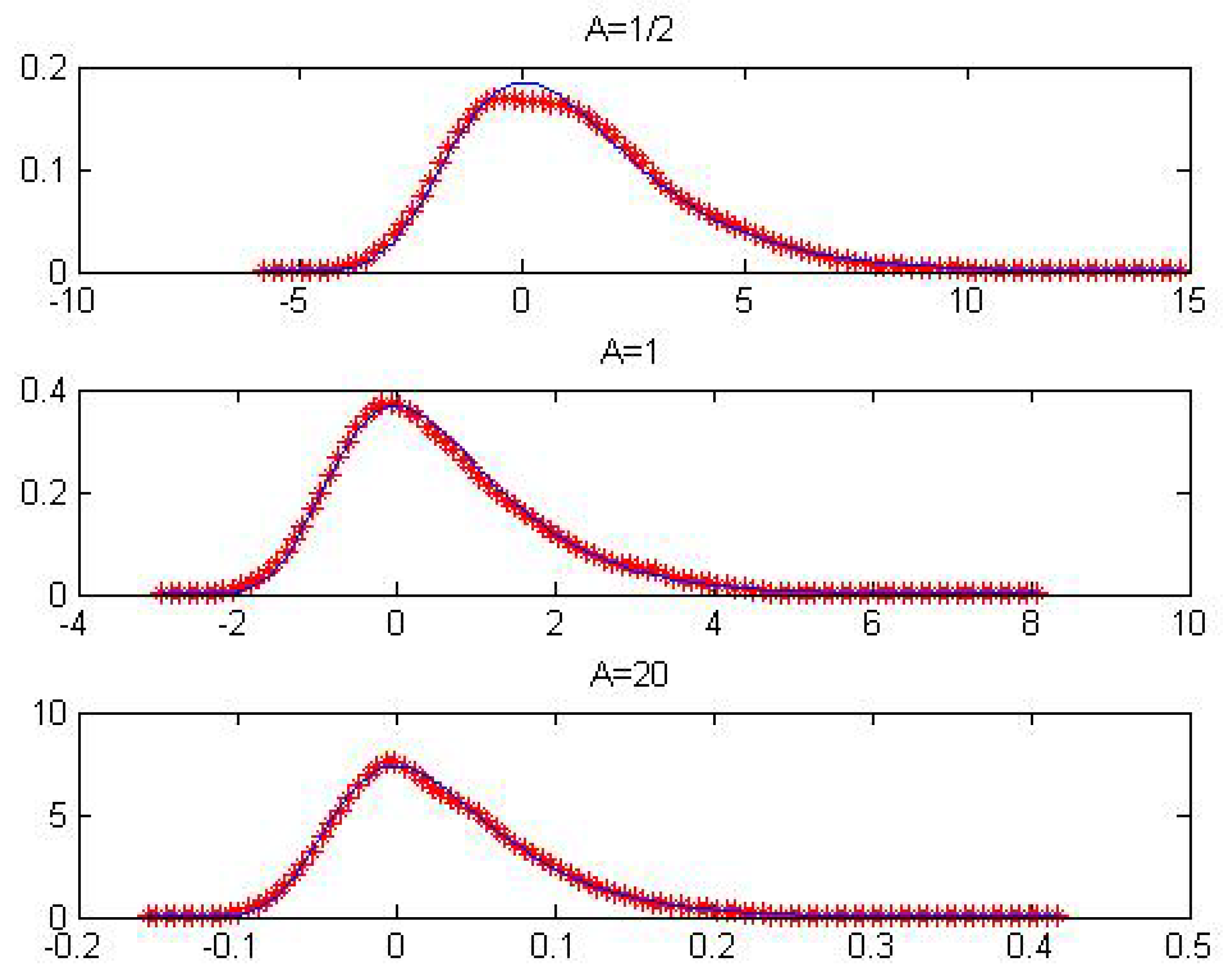
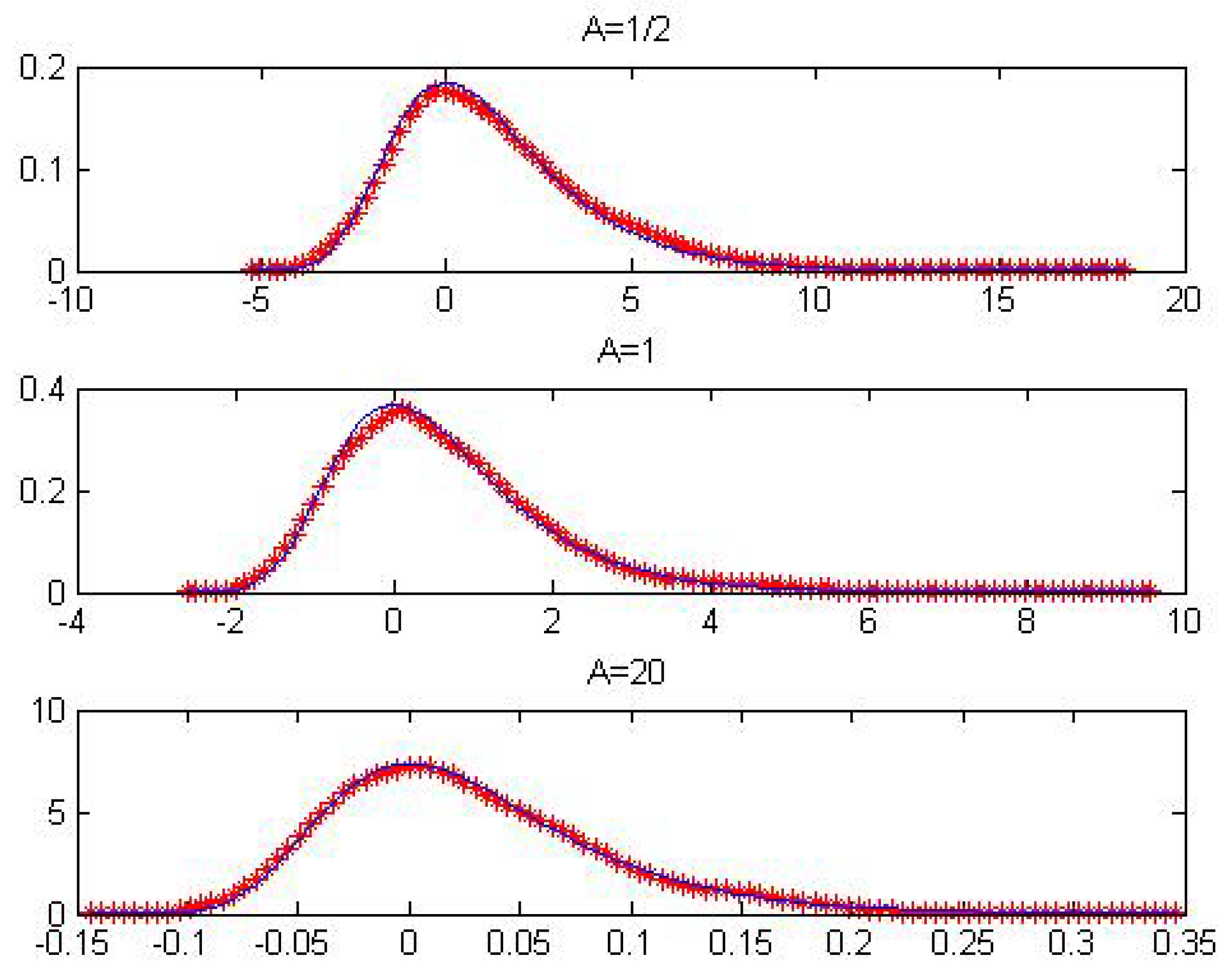
Here, we choose $A=\frac{1}{2},1,20$, respectively. The results are presented in

Table 2. Uniform convergence rate and convergence order for uniform distribution.

$\mathit{A}=1/2$			$\mathit{A}=1$			$\mathit{A}=20$
$\mathit{n}$	Rate	Order	$\mathit{n}$	Rate	Order	$\mathit{n}$	Rate	Order
2	0.3078		1	0.3679		1	0.3679
10	0.00516	$-1.1097$	10	0.0246	$-1.1748$	10	0.0192	$-1.2824$
${10}^2$	0.0048	$-1.0314$	${10}^2$	0.0024	$-1.0107$	${10}^2$	0.0018	$-1.0280$
${10}^3$	$4.7561\times {10}^{-4}$	$-1.0040$	${10}^3$	$2.3545\times {10}^{-4}$	$-1.0083$	${10}^3$	$1.8402\times {10}^{-4}$	$-0.9904$
${10}^4$	$4.7526\times {10}^{-5}$	$-1.0003$	${10}^4$	$2.3535\times {10}^{-5}$	$-1.0002$	${10}^4$	$1.8395\times {10}^{-5}$	$-1.0002$

and

Table 3. Uniform convergence rate and convergence order for exponential distribution.

$\mathit{A}=1/2$			$\mathit{A}=1$			$\mathit{A}=20$
$\mathit{n}$	Rate	Order	$\mathit{n}$	Rate	Order	$\mathit{n}$	Rate	Order
2	0.1617		1	0.3679		1	0.3679
10	0.0280	$-1.0896$	10	0.0279	$-1.1195$	10	0.0248	$-1.1718$
${10}^2$	0.0027	$-1.0136$	${10}^2$	0.0027	$-1.0107$	${10}^2$	0.0027	$-1.0280$
${10}^3$	$2.7070\times {10}^{-4}$	$-1.0013$	${10}^3$	$2.7070\times {10}^{-4}$	$-1.0083$	${10}^3$	$2.5762\times {10}^{-4}$	$-0.9904$
${10}^4$	$2.7060\times {10}^{-5}$	$-1.0002$	${10}^4$	$2.7060\times {10}^{-5}$	$-1.0002$	${10}^4$	$1.9649\times {10}^{-5}$	$-1.0002$

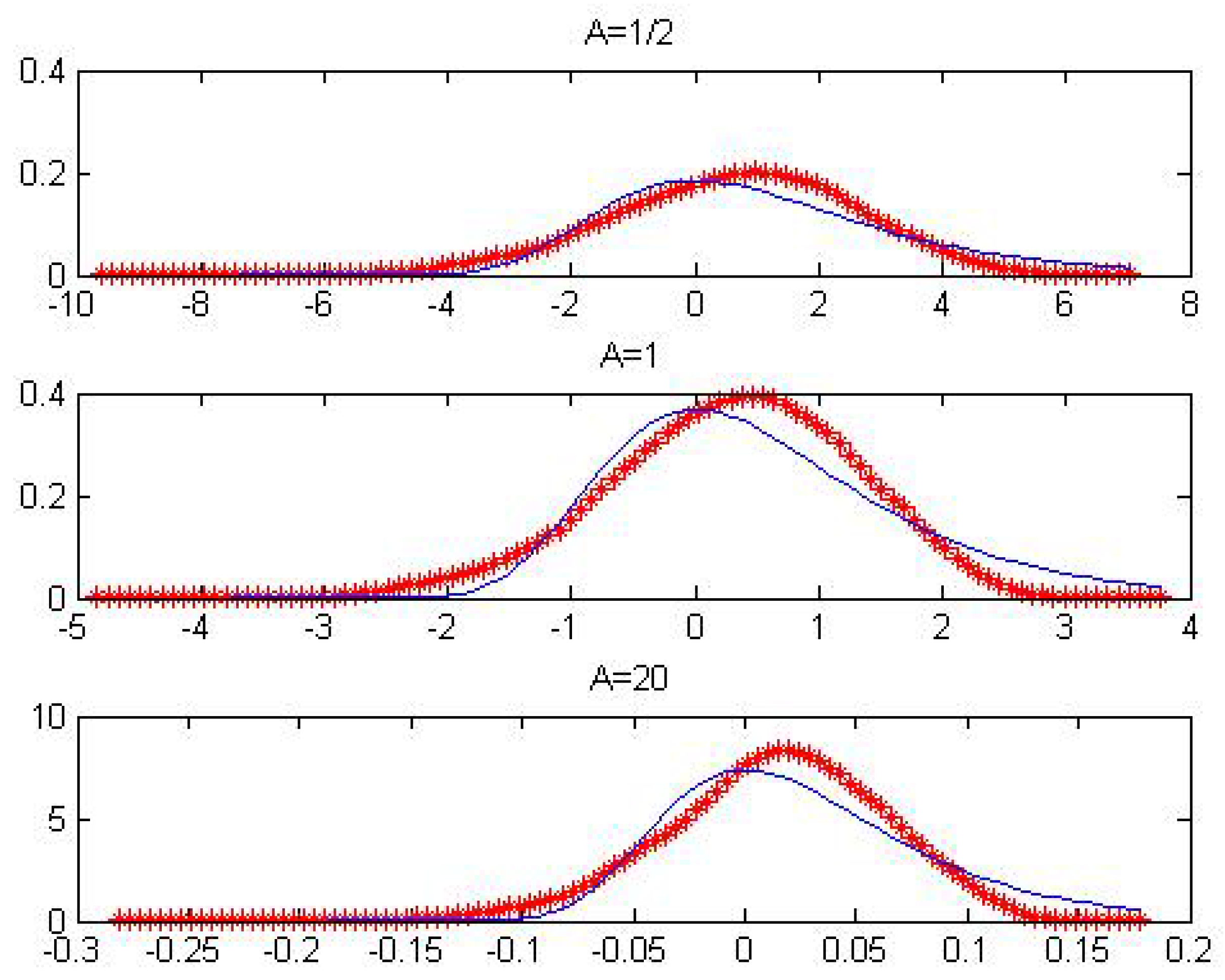
and Figure 1, Figure 2 and Figure 3. Note that the second derivative of Cauchy distribution function is unbounded on $D_n$; consequently, this kind of distribution could not converge to $G_A(x)$ uniformly in this domain. For this reason, we only test the asymptotic behavior of extremes by feedback sketch. The results are presented in Figure 3. These results suggest that the uniform convergence rate is of order $O(\frac{1}{n})$ for different A as predicted by Theorem 1. Figure 1, Figure 2 and Figure 3 show that the asymptotic density is essentially coincident with the extreme value density $G_A^{\prime }(x)$ as posed in Remark 1.

6. Conclusions

In this paper we have provided the analysis of deriving the limiting distributions and convergence rates for the minimum-maximum model. Under the framework of this model, we considered the i.i.d. random sequence and the stationary random sequence satisfying the strong mixing condition respectively. Without specifying the form of the distribution functions of the two sequences, our results yield that the limiting distribution of $M_n$ converges to a non-standard Gumbel distribution. For the distribution functions having continuous and bounded first derivatives, the limiting distribution has the convergence properties as shown in Theorem 4. In particular, for the distribution functions having continuous and bounded second derivates, our result reveals a uniform convergence rate of $O(n^{-1})$.