A Novel Integral Equation for the Riemann Zeta Function and Large t-Asymptotics

Abstract

Based on the new approach to Lindelöf hypothesis recently introduced by one of the authors, we first derive a novel integral equation for the square of the absolute value of the Riemann zeta function. Then, we introduce the machinery needed to obtain an estimate for the solution of this equation. This approach suggests a substantial improvement of the current large $t-$asymptotics estimate for $\zeta \left(\frac{1}{2}+it\right)$.

1. Introduction

It is well known that the leading asymptotics for large t of $\zeta \left(s\right)$ can be expressed in terms of a transcendental sum,

$$\zeta \left(s\right)\sim \sum _{m=1}^{\left[t\right]}\frac{1}{m^s},s=\sigma +it,0<\sigma <1,t\to \infty ,$$

(1)

where throughout this paper [A] denotes the integer part of the positive number A. Lindelöf’s hypothesis, one of the most important open problems in the history of mathematics, states that for $\sigma =1/2$, this sum is of order $O\left(t^{\epsilon }\right)$ for any $\epsilon >0$.

The sum of the rhs of (1) is a particular case of an exponential sum. Pioneering results for the estimation of such sums were obtained in 1916 using methods developed by Weyl [1], and Hardy and Littlewood [2], when it was shown that $\zeta (1/2+it)=O\left(t^{1/6+\epsilon }\right)$. In the last 100 years some slight progress was made using the ingenious techniques of Vinogradov [3]. Currently, the best result is due to Bourgain [4] who has been able to reduce the exponent factor to $13/84\approx 0.155$.

It is interesting that, in contrast to the usual situation in asymptotics where higher order terms in an asymptotic expansion are more complicated, the higher order terms of the asymptotic expansion of $\zeta \left(s\right)$ can be computed explicitly. Siegel, in his classical paper [5] presented the asymptotic expansion of $\zeta \left(s\right)$ to all orders in the important case of $x=y=\sqrt{t/2\pi }$. In [6], analogous results are presented for anyx and y valid to all orders. A similar result for the Hurwitz zeta function is presented in [7]. Some of the results of [6] are used in [8] and the latter results are useful for the estimates presented in this paper.

A major obstacle in trying to prove Lindelöf’s hypothesis via the estimation of relevant exponential sums is that in estimates one “loses” something (the more powerful the technique, the less the loss). Here we follow the new formalism for analysing the large t-asymptotics of the Riemann zeta function, introduced in [9]. For the sake of clarity of presentation we restrict our attention to the case $\sigma =1/2$.

We start with the following integral equation derived in Equation (1.6) of [9]:

$$\begin{array}{cc}\hfill \frac{t}{\pi }& {\oint }_{-t^{{\delta }_1-1}}^{1+t^{{\delta }_4-1}}\Re \left\{\frac{\mathsf{\Gamma }(it-i\tau t)}{\mathsf{\Gamma }(1/2+it)}\mathsf{\Gamma }(1/2+i\tau t)\right\}{\left|\zeta (1/2+i\tau t)\right|}^2\mathrm{d}\tau +\mathcal{G}(1/2,t)\hfill \\ \hfill +& O\left(e^{-\pi t^{{\delta }_{14}}}\right)=0,t\to \infty ,\hfill \\ & {\delta }_1>0,{\delta }_4>0,{\delta }_{14}=\min ({\delta }_1,{\delta }_4),\hfill \end{array}$$

(2)

where $\mathsf{\Gamma }\left(z\right)$ denotes the usual gamma function, the principal value integral is defined with respect to $\tau =1$ and $\mathcal{G}(1/2,t)$ satisfies the estimate

$$\mathcal{G}(1/2,t)=lnt+O\left(1\right),t\to \infty .$$

(3)

In [9] the computation of the large t asymptotics of (2) is obtained by first splitting the interval $[-t^{{\delta }_1-1},1+t^{{\delta }_4-1}]$ into the following four subintervals:

$$\begin{array}{c}{L}_1=[-t^{{\delta }_1-1},t^{-1}],L_2=[t^{-1},t^{{\delta }_2-1}],\hfill \\ L_3=[t^{{\delta }_2-1},1-t^{{\delta }_3-1}],L_4=[1-t^{{\delta }_3-1},1+t^{{\delta }_4-1}],\hfill \end{array}$$

(4)

with ${\delta }_j\in (0,1),j=1,2,3,4$. We employ the same splitting in (2) and hence the asymptotic evaluation of (2) reduces to the analysis of the four integrals,

$$\begin{array}{cc}\hfill I_j\left(t\right)=& \frac{t}{\pi }{\oint }_{L_j}\Re \left\{\frac{\mathsf{\Gamma }(it-i\tau t)}{\mathsf{\Gamma }(1/2+it)}\mathsf{\Gamma }(1/2+i\tau t)\right\}{\left|\zeta (1/2+i\tau t)\right|}^2\mathrm{d}\tau ,t>0,\hfill \end{array}$$

(5)

where $I_1$, $I_2$, $I_3$, $I_4$ also depend on ${\delta }_1$, ${\delta }_2$, $({\delta }_2,{\delta }_3)$, $({\delta }_3,{\delta }_4)$, respectively, $L_1,L_2,L_3,L_4$ are defined in (4), and the principal value integral is needed only for $I_4$.

Organisation of the Paper

In Section 2 we derive a linear integral equation for ${\left|\zeta \left(s\right)\right|}^2$. This equation is given by (23) where $S_4^P$ and $S_4^{SD}$ are defined by (18) and (19), respectively.

In Section 3 we present the methodology for deriving the main result of this paper, namely the linear Volterra-type integral equation for ${\left|\zeta \left(s\right)\right|}^2$ given by Equation (8) below. In this connection, we first estimate the double sum $S_4^P$ appearing in the linear integral Equation (23):

$$\Re \left\{S_4^P(t,{\delta }_3)\right\}=O\left(t^{\frac{{\delta }_3}{2}}lnt\right),t\to \infty .$$

(6)

Then, we present heuristic arguments regarding the estimation of $S_4^{SD}$, which suggest that

$$S_4^{SD}=O\left(t^{\frac{1}{3}-\frac{{\delta }_3}{2}}{(lnt)}^2\right)+O\left(t^{\frac{{\delta }_3}{2}}lnt\right),t\to \infty .$$

(7)

Replacing in (23) $S_4^P$ and $S_4^{SD}$ by (6) and (7), for $0<{\delta }_2<1/2$ and ${\delta }_3=1/3$, we find the main result of the paper:

$$\begin{array}{cc}\hfill {\left|\zeta \left(\frac{1}{2}+it\right)\right|}^2& =\frac{1}{\pi }{\int }_{t^{{\delta }_2}}^{t-t^{1/3}}\mathcal{K}(\rho ,t){\left|\zeta \left(\frac{1}{2}+i\rho \right)\right|}^2\mathrm{d}\rho +O\left(t^{\frac{1}{6}}{(lnt)}^2\right),t\to \infty ,\hfill \end{array}$$

(8)

where the kernel $K(\rho ,t)$ is given by

$$\mathcal{K}(\rho ,t)=\Re \left\{\frac{\mathsf{\Gamma }(it-i\rho )}{\mathsf{\Gamma }(1/2+it)}\mathsf{\Gamma }(1/2+i\rho )\right\}.$$

(9)

For the rigorous derivation of (7) we make crucial use of some of the results of [10]. For completeness of presentation, the relevant results of [10] are reviewed in Section 3.

In Section 4 we derive (7). This derivation is based on the following: first, on a lemma for partial summation in two dimensions, which is crucial for the analysis of some parts of the sum $S_4^{SD}$. Second, on the asymptotic estimates of the function $E_4^{SD}(t,\delta )$ appearing in the definition of $S_4^{SD}$ which are given in [11]. Third, on the splitting of $S_4^{SD}$ into three cases involving certain sums denoted by $S^{\left(i\right)}$, $S^{\left(ii\right)}$, $S^{\left(iii\right)}$. Relatively straightforward estimates yield that both $S^{\left(ii\right)}$ and $S^{\left(iii\right)}$ are $O\left(t^{\frac{\delta }{2}}lnt\right),t\to \infty$. The estimation of $S^{\left(i\right)}$ is quite complicated; details are given in Section 4.3.

Section 5 summarizes the basic results in this paper and discusses future directions.

2. Derivation of a Linear Integral Equation for ${\left|\mathbf{\zeta }\left(\mathbf{s}\right)\right|}^{\mathbf{2}}$

The main result of this section is the linear integral Equation (23) which is obtained from (2) by computing the contribution of the integrals ${\left\{I_j\right\}}_1^4$. In this direction, we first recall the estimates for $I_1$ and $I_2$, and then we introduce a methodology that computes explicitly the leading asymptotic behaviour of $I_4$. In addition, this methodology avoids the need to compute the asymptotics of $I_3$.

2.1. The Contribution of $I_1$ and $I_2$

Using Lemma 4.1 of [9], it can be shown that for ${\delta }_1$ sufficiently small, $I_1$ satisfies the estimate

$$I_1(t,{\delta }_1)=O\left(t^{-1/2+\frac{4}{3}{\delta }_1}\right),t\to \infty .$$

(10)

Furthermore, by employing the classical estimates of Atkinson, and following the steps of Lemma 4.2 of [9], it can be shown that that $I_2$ satisfies the estimate

$$I_2(t,{\delta }_2)=O\left(t^{-\frac{1}{2}+{\delta }_2}lnt\right),0<{\delta }_2<1,t\to \infty .$$

(11)

Thus, for sufficiently small ${\delta }_1$ and ${\delta }_2$ Equations (10) and (11) yield

$$I_1=o\left(1\right)\mathrm{and}{I}_2=o\left(1\right),t\to \infty .$$

(12)

2.2. The Contribution of the Leading Order Term of $I_4$

Let ${\tilde{I}}_4$ denote the contribution of the leading order term of $I_4$. This term is defined by replacing $\zeta \left(s\right)$ with the leading term of its large t-asymptotics in (5) for $j=4$. Using the change of variables $\tau =1-\frac{x}{t}$, ${\tilde{I}}_4$ becomes

$${\tilde{I}}_4(t,{\delta }_3,{\delta }_4)=\frac{1}{\pi }{\oint }_{-t^{{\delta }_4}}^{t^{{\delta }_3}}\Re \left\{\mathsf{\Gamma }\left(ix\right)\frac{\mathsf{\Gamma }(1/2+it-ix)}{\mathsf{\Gamma }(1/2+it)}\right\}{\left|\tilde{\zeta }(1/2+it-ix)\right|}^{2}dx,$$

(13)

where the principal value integral is with respect to $x=0$, and

$$|\tilde{\zeta }{(1/2+it-ix)|}^2=\sum _{m_1=1}^{\left[t\right]}\sum _{m_2=1}^{\left[t\right]}\frac{1}{m_1^s{m}_2^{\overline{s}}}{\left(\frac{m_1}{m_2}\right)}^{ix},s=\frac{1}{2}+it.$$

(14)

Thus, we obtain the following expression for the leading behaviour of $I_4$:

$$\begin{array}{cc}\hfill & {\tilde{I}}_4(t,{\delta }_3,{\delta }_4)=\Re \left\{\sum _{m_1=1}^{\left[t\right]}\sum _{m_2=1}^{\left[t\right]}\frac{1}{m_1^s}\frac{1}{m_2^{\overline{s}}}{J}_4\left(\sigma ,t,{\delta }_2,{\delta }_3,\frac{m_1}{m_2}\right)\right\},s=\frac{1}{2}+it,\hfill \end{array}$$

(15)

where $J_4$ is defined by

$$\begin{array}{c}{J}_4\left(t,{\delta }_3,{\delta }_4,\frac{m_1}{m_2}\right)=\frac{1}{\pi }{\oint }_{-t^{{\delta }_4}}^{t^{{\delta }_3}}\mathsf{\Gamma }\left(ix\right)\frac{\mathsf{\Gamma }(1/2+it-ix)}{\mathsf{\Gamma }(1/2+it)}{\left(\frac{m_1}{m_2}\right)}^{ix}\mathrm{d}x,\hfill \\ t>0,0<{\delta }_3<1,0<{\delta }_4<1,m_j=1,2,\dots ,\left[t\right],\hfill \end{array}$$

(16)

with the principal value integral defined with respect to $x=0$.

Theorem 6.1 of [9] gives the estimate

$$\begin{array}{cc}\hfill {\tilde{I}}_4(t,{\delta }_3,{\delta }_4)& =\left\{-\sum _{m_1=1}^{\left[t\right]}\sum _{m_2=1}^{\left[t\right]}\frac{1}{m_1^s{m}_2^{\overline{s}}}+2\Re \left\{S_4^P\right\}+\Re \left\{S_4^{SD}\right\}\right\}\left[1+O\left(t^{2{\delta }_{34}-1}\right)\right],t\to \infty \hfill \\ & s=\frac{1}{2}+it,0<{\delta }_3<\frac{1}{2},0<{\delta }_4<\frac{1}{2},{\delta }_{34}=max\{{\delta }_3,{\delta }_4\},\hfill \end{array}$$

(17)

where $S_4^P$ and $S_4^{SD}$ are defined as follows:

$$S_4^P(t,{\delta }_3)=\underset{m_1,m_2\in M_4}{\sum \sum }\frac{1}{m_1^s{m}_2^{\overline{s}}}{e}^{-\frac{i{m}_2}{m_1}t}$$

(18)

with

$$M_4:=M_4({\delta }_3,t)=\left\{m_j=1,\dots ,\left[t\right],j=1,2,\frac{m_1}{m_2}\in (t^{1-{\delta }_3},t)\right\},$$

and

$$S_4^{SD}(t,{\delta }_3)=\sum _{m_1=1}^{\left[t\right]}\sum _{m_2=1}^{\left[t\right]}\frac{1}{m_1^s{m}_2^{\overline{s}}}{E}_4^{SD}(t,{\delta }_3);$$

(19)

$E_4^{SD}$ satisfies the asymptotic estimate

$$E_4^{SD}\sim -\sqrt{\frac{2}{\pi }}{e}^{\frac{i\pi }{4}}{t}^{-\frac{{\delta }_3}{2}}{e}^{-i{t}^{{\delta }_3}}{t}^{i({\delta }_3-1)t^{{\delta }_3}}\frac{1}{ln\left(\frac{m_2}{m_1}{t}^{1-{\delta }_3}\right)}{\left(\frac{m_1}{m_2}\right)}^{i{t}^{{\delta }_3}},t\to \infty ,$$

(20)

when $\frac{m_2}{m_1}{t}^{1-{\delta }_3}\ne 1$.

Remark 1.

According to the analysis of [9], the derivation of (17) involves the computation of the contribution of an integral along the so-called Hankel contour. The function $S_4^P$ is related with the contribution of the pole $w_P=-i\frac{m_2}{m_1}{t}^{1-{\delta }_3}$ and $S_4^{SD}$ is related with the contribution of the Hankel contour after deforming it so that it passes through the point of steepest descent $w_{SD}=-i$. Hence, we call $S_4^P$ and $S_4^{SD}$ as the Pole and Steepest Descent contribution, respectively.

2.3. The Contribution of $I_3$

Let $I_3$ be defined by (5), with $j=3$. By making the change of variables $\rho =t\tau$, we obtain

$$\begin{array}{c}\hfill I_3(t,{\delta }_2,{\delta }_3)=\frac{1}{\pi }{\int }_{t^{{\delta }_2}}^{t-t^{{\delta }_3}}\Re \left\{\frac{\mathsf{\Gamma }(it-i\rho )}{\mathsf{\Gamma }(1/2+it)}\mathsf{\Gamma }(1/2+i\rho )\right\}{\left|\zeta (1/2+i\rho )\right|}^2\mathrm{d}\rho .\end{array}$$

(21)

2.4. A Volterra-Type Integral Equation

It is shown in Appendix A that the first term of the rhs of (17) is the leading asymptotic term of ${\left|\zeta \right|}^2$. Hence, (17) becomes

$$\begin{array}{c}\hfill {\tilde{I}}_4(t,{\delta }_3,{\delta }_4)\sim -{\left|\zeta \left(s\right)\right|}^2+2\Re \left\{S_4^P\right\}+\Re \left\{S_4^{SD}\right\},s=\frac{1}{2}+it,t\to \infty .\end{array}$$

(22)

By replacing in (2), $I_1$ and $I_2$ by (12), $I_3$ by (21) and $I_4$ by (22) we obtain the following Volterra-type integral equation:

$$\begin{array}{cc}\hfill {\left|\zeta (1/2+it)\right|}^2& =\frac{1}{\pi }{\int }_{t^{{\delta }_2}}^{t-t^{{\delta }_3}}\Re \left\{\frac{\mathsf{\Gamma }(it-i\rho )}{\mathsf{\Gamma }(1/2+it)}\mathsf{\Gamma }(1/2+i\rho )\right\}{\left|\zeta (1/2+i\rho )\right|}^2\mathrm{d}\rho \hfill \\ & +2\Re \left\{S_4^P\right\}+\Re \left\{S_4^{SD}\right\}+lnt+O\left(1\right),t\to \infty ,\hfill \end{array}$$

(23)

where $S_4^P$ and $S_4^{SD}$ are given in (18) and (19), respectively.

3. The Methodology for Deriving the Integral Equation (8)

In this section we derive Equation (6) and we also provide heuristic arguments for supporting the validity of Equation (7). The employment of the estimates (6) and (7), evaluated at ${\delta }_3=1/3$, in Equation (23) yields (8).

3.1. An Estimate for $S_4^P$

In order to estimate the sum $S_4^P$, we use (1.30) of [9], namely (See Appendix B)

$$S_3(t,{\delta }_3)=S_4^P(t,{\delta }_3)\left[1+O\left(t^{2{\delta }_3-1}\right)\right],t\to \infty ,$$

(24)

with

$$S_3(t,{\delta }_3)=\underset{(m_1,m_2)\in M_3}{\sum \sum }\frac{1}{m_2^{\overline{s}}{(m_1+m_2)}^s},s=\frac{1}{2}+it,$$

(25)

and $M_3$ is defined by

$$M_3:=M_3({\delta }_3,t)=\left\{m_j=1,\dots ,\left[t\right],j=1,2,\frac{m_2}{m_1}<\frac{1}{t^{1-{\delta }_3}-1}\right\}.$$

(26)

Using results of [6], it is shown in Theorem 5.1 of [8] that

$$S_3(t,{\delta }_3)=O\left(t^{\frac{{\delta }_3}{2}}lnt\right),t\to \infty .$$

(27)

Thus, (6) follows.

3.2. An Estimate for $S_4^{SD}$

The definition of $S_4^{SD}$, given in (19), implies

$$S_4^{SD}=O\left(\frac{1}{t^{\frac{{\delta }_3}{2}}}\left|\sum _{m_1=1}^{\left[t\right]}\sum _{m_2=1}^{\left[t\right]}\frac{1}{m_1^{\frac{1}{2}+i(t-t^{{\delta }_3})}{m}_2^{\frac{1}{2}-i(t-t^{{\delta }_3})}}\frac{1}{ln\left(\frac{m_2}{m_1}{t}^{1-{\delta }_3}\right)}\right|\right).$$

(28)

In order to estimate the sum $S_4^{SD}$, we employ the classical techniques of [10,12,13,14]. These techniques can be used for the estimation of the sums of the form

$$\underset{1<m<n<\left[t\right]}{\sum \sum }\frac{1}{m^{\frac{1}{2}+it}{n}^{\frac{1}{2}-it}}.$$

In this connection we recall the following well known result (see, for example, Theorem 5.12 of [13]):

$$\sum _{n=1}^{\left[t\right]}\frac{1}{n^{\frac{1}{2}+it}}=O\left(t^{\frac{1}{6}}lnt\right),t\to \infty .$$

(29)

The above result can be further improved, see, for example, Theorem 5.18 of [13]:

$${\left|\sum _{n=1}^{\left[t\right]}\frac{1}{n^{\frac{1}{2}+it}}\right|}^2=O\left(t^{\frac{1}{3}}\right),t\to \infty .$$

(30)

Using similar arguments, it is straightforward to show that

$${\left|\sum _{n=1}^{\left[t\right]}\frac{1}{n^{\frac{1}{2}+i(t-t^{{\delta }_3})}}\right|}^2=O\left(t^{\frac{1}{3}}\right),t\to \infty .$$

(31)

It turns out that the techniques of [10] can be directly applied to estimating sums involving the lhs of (31). In this way it can be shown that

$$\sum _{m_1=1}^{\left[t\right]}\sum _{m_2=1}^{\left[t\right]}\frac{1}{m_1^{\frac{1}{2}+i(t-t^{{\delta }_3})}{m}_2^{\frac{1}{2}-i(t-t^{{\delta }_3})}}=O\left(t^{\frac{1}{3}}{(lnt)}^2\right),t\to \infty .$$

The sum in the rhs of (28), in comparison to the above sum contains the extra term $\frac{1}{ln\left(\frac{m_2}{m_1}{t}^{1-{\delta }_3}\right)}$. Fortunately, this term satisfies the properties needed for the partial summation procedure. Actually, a slight modification of the partial summation technique used in [10] suggests the estimate (7).

We note that the second term of the rhs of (7) is identical with the estimate of (6). This is due to the fact that the estimation of $S_4^{SD}$ involves the splitting of the relevant set of the summation of in three parts, and in one of these parts the summand has the form of the summand of (18).

3.3. Review of Techniques for Estimating Euler-Zagier Double Sums

We summarise some of the techniques used in [10] that will be needed in the estimation of the sum $S_4^{SD}$. In what follows we use the terminology of [10].

In [10] estimates of the Euler-Zagier double sums are obtained by employing techniques from [12,14]. Indeed, letting $s_j={\sigma }_j+i{t}_j$, with $0\le {\sigma }_j<1,j=1,2$ and $|t_j|\sim c_{j}t$, for some positive constants $c_j$, estimates as $t\to \infty$ are derived for sums of the form

$$\sum _{1\le m<n}{\displaystyle \frac{1}{m^{s_1}}}{\displaystyle \frac{1}{n^{s_2}}}.$$

A special case of Theorem 1.1 in [10] yields

$$\sum _{1\le m<n}{\displaystyle \frac{1}{m^{\frac{1}{2}+it}}}{\displaystyle \frac{1}{n^{\frac{1}{2}+it}}}=O\left(t^{\frac{1}{3}}{(lnt)}^2\right).$$

The above result, as well as the estimates of Theorem 1.1 therein, provide a ‘sharp’ generalisation for double sums of the classical result for the single sum of Theorem 5.12 in [13]. In this sense, the results of [10] improve significantly the analogous results of [15].

Here we are interested only on the part of the analysis of [10] concerning the sums of the form

$$S_1=\sum _{1\le m<n<t}{\displaystyle \frac{1}{m^{s_1}}}{\displaystyle \frac{1}{n^{s_2}}},$$

and in particular for the case that ${\sigma }_1={\sigma }_2=1/2$. The above sum is estimated by splitting it into two classes of sums:

$$S_1=\sum _{j=1}^{\left[\frac{ln2t}{ln2}\right]}\left[T\left(2^{-j}t\right)+U\left(2^{-j}t\right)\right],$$

where

$$T\left(M\right)=\sum _{M<m<n\le 2M}{\displaystyle \frac{1}{m^{s_1}}}{\displaystyle \frac{1}{n^{s_2}}}\mathrm{and}U\left(M\right)=\sum _{1\le m\le M}{\displaystyle \frac{1}{m^{s_1}}}\sum _{M<n\le 2M}{\displaystyle \frac{1}{n^{s_2}}}.$$

The estimation of the sum $U\left(M\right)$ is straightforward since it can be reduced to the estimation of a single sum; this is given by employing the Theorem 5.12 of [13], namely

$$\sum _{1\le m\le M}{\displaystyle \frac{1}{m^{1/2+it}}}=O\left(t^{\frac{1}{6}}lnt\right)\mathrm{and}\sum _{M<m\le 2M}{\displaystyle \frac{1}{n^{1/2+it}}}=O\left(t^{\frac{1}{6}}\right).$$

Thus,

$$\sum _{j=1}^{\left[\frac{ln2t}{ln2}\right]}U\left(2^{-j}t\right)=O\left(t^{\frac{1}{3}}{(lnt)}^2\right),t\to \infty .$$

The estimation of the sum $T\left(M\right)$ is more elaborate and is based on Lemmas 3.1–3.5, therein. Lemma 3.1 appears in [14], Lemmas 3.2–3.4 appear in [12], and Lemma 3.5 is a variation of the classical and widely used partial summation technique (see for example [13,14]).

Since the latter Lemma plays an important role in our analysis we find it helpful to restate it:

Lemma 1

(Lemma 3.5 in [10]). Let M and N be positive integers such that $M<N$, $f(x,y)$ be a $C^2$-function on $[M,N]\times [M,N]$, $g(m,n)$ be an arithmetical function on the same domain, and

$$G(x,y)=\underset{x<m\le n\le y}{\sum \sum }g(m,n).$$

Suppose that

$$\left|G(x,y)\right|\le G,|f_x(x,y)|\le {\kappa }_1,|f_y(x,y)|\le {\kappa }_2,\left|f_{xy}(x,y)\right|\le {\kappa }_3,$$

for some positive constants $G,{\kappa }_1,{\kappa }_2,{\kappa }_3$, and for any $M\le x,y\le N$. Then, we have

$$\left|\underset{M<m\le n\le N}{\sum \sum }f(m,n)g(m,n)\right|\le G\left[f(M,N)+({\kappa }_1+{\kappa }_2)(N-M)+{\kappa }_3{(N-M)}^2\right].$$

(32)

In order to estimate the sum $T\left(M\right)$ the set of summation is divided in three regions corresponding to the following three cases:

(a)

$M<t^{\frac{1}{3}}$

(b)

$t^{\frac{1}{3}}<M<t^{\frac{2}{3}}$

(c)

$t^{\frac{2}{3}}<M<t$.

For case (a) it is sufficient to observe that $T\left(M\right)=O\left(M\right)$, which yields

$$\sum _{j=\left[\frac{2}{3}\frac{lnt}{ln2}\right]}^{\left[\frac{ln2t}{ln2}\right]}T\left(2^{-j}t\right)=O\left(t^{\frac{1}{3}}lnt\right),t\to \infty .$$

For case (c) Lemma 3.4 is used to treat the oscillatory part of the sum, i.e., it is shown that ${\displaystyle \sum _{M<m<n\le 2M}{\displaystyle \frac{1}{m^{i{t}_1}}}{\displaystyle \frac{1}{n^{i{t}_2}}}=O(tlnt)}$. Then, applying partial summation using Lemma 3.5 which shows that $T\left(M\right)=O\left(\frac{1}{M}tlnt\right)$, it follows that

$$\sum _{j=1}^{\left[\frac{1}{3}\frac{lnt}{ln2}\right]}T\left(2^{-j}t\right)=O\left(t^{\frac{1}{3}}{(lnt)}^2\right),t\to \infty .$$

Case (b) is conceptually the same with case (c) but involves more technicalities: Lemmas 3.1–3.3 are used to treat the oscillatory part of the sum, i.e., to show that ${\displaystyle \sum _{M<m<n\le 2M}{\displaystyle \frac{1}{m^{i{t}_1}}}{\displaystyle \frac{1}{n^{i{t}_2}}}=O\left(M{t}^{\frac{1}{3}}{(lnt)}^{\frac{1}{2}}\right)}$. Then, applying partial summation by using Lemma 3.5 in order to obtain that $T\left(M\right)=O\left(t^{\frac{1}{3}}{(lnt)}^{\frac{1}{2}}\right)$, it follows that

$$\sum _{j=\left[\frac{1}{3}\frac{lnt}{ln2}\right]}^{\left[\frac{2}{3}\frac{lnt}{ln2}\right]}T\left(2^{-j}t\right)=O\left(t^{\frac{1}{3}}{(lnt)}^{\frac{3}{2}}\right),t\to \infty .$$

Summarising the above results it follows that

$$S_1=\sum _{1\le m<n<t}{\displaystyle \frac{1}{m^{s_1}}}{\displaystyle \frac{1}{n^{s_2}}}=O\left(t^{\frac{1}{3}}{(lnt)}^2\right),t\to \infty .$$

(33)

Remark 2.

From the above analysis it follows that it is much more complicated to estimate the sums of the form $T\left(M\right)$ in comparison to those of the form $U\left(M\right)$; the latter ones correspond to set of summations which can be decoupled, whereas the set of summations corresponding to the former ones cannot be decoupled. The latter observation necessitates the use of the Lemma 3.5 in [10], which is related with the partial summation technique. The sets of summation in our work are more complicated, requiring more general forms of that Lemma. In this connection, in Section 4.1 we state a general form of Abel’s summation formula for double sums; its proof is presented in [11].

4. Derivation of the Estimate (7)

In what follows we let ${\delta }_3=\delta$, and throughout the rest of the paper we have $s=1/2+it$.

In order to derive (7), we split the sum $S_4^{SD}$ in three different sums $S^{\left(i\right)}$, $S^{\left(ii\right)}$, $S^{\left(iii\right)}$, in accordance with the analysis of Section 4.2, below. We analyse these three sums in Section 4.3:

• The estimation of $S^{\left(iii\right)}$ is straightforward.
• The estimation of $S^{\left(ii\right)}$ involves the use of partial summation technique described in [14].
• The estimation of $S^{\left(i\right)}$ is based on the the analysis of [10], but some of the parts of the sum require the use of a partial summation which is more general than the one derived in [10]. In this direction, we will use a lemma on Abel’s summation in two dimensions stated below.

4.1. A Lemma for Partial Summation in Two Dimensions

Lemma 3.5 of [10] is a two-dimensional form of the so-called Abel’s summation formula, see Appendix C. The difficulty appearing in the proof of Lemma 3.5 of [10] is due to the fact that the set of summation is given by an expression which does not allow the double sum to be decoupled in two single sums. In the separable case the simple form of the Abel’s summation formula for double sums is given in Lemma A1, and is straightforward to derive it by applying twice (A1). However, for our analysis we need to generalise Lemma 3.5 of [10]. This generalisation is given by Lemma 2 below, whose proof is given in [11]. It is this form of Abel’s summation formula for double sums that is needed for the analysis of the sums (3b) and (4b) appearing in the sum $S_2^{\left(i\right)}$, which is analysed in Section 4.3.

Lemma 2.

Let $\theta (·)$ be a linear function and $\varphi (·)$ be its inverse. Particular such functions are $\theta \left(x\right)=t^{\delta -1}x$, $\varphi \left(x\right)=t^{1-\delta }x$. Let $M<N$ be positive integers and $f(x,y)$ be a $C^2$-function on $\left[\theta \right(M),\theta (N\left)\right]\times [M,N]$, $g(m,n)$ be an arithmetical function on the same domain, and

$$G(x,y)=\underset{x<\varphi \left(m\right)<n\le y}{\sum \sum }g(m,n).$$

Suppose that

$$\left|G(x,y)\right|\le G,|f_x(x,y)|\le {\kappa }_1,|f_y(x,y)|\le {\kappa }_2,\left|f_{xy}(x,y)\right|\le {\kappa }_3,$$

for some positive constants $G,{\kappa }_1,{\kappa }_2,{\kappa }_3$, and for any $(x,y)\in \left[\theta \right(M),\theta (N\left)\right]\times [M,N]$.Then, we have

$$\begin{array}{cc}\hfill & \left|\underset{M<\varphi \left(m\right)<n\le N}{\sum \sum }f(m,n)g(m,n)\right|\hfill \\ \hfill \le & G\left[f\left(\theta \left(M\right),N\right)+{\kappa }_1\left(\theta \left(N\right)-\theta \left(M\right)\right)+{\kappa }_2(N-M)+{\kappa }_3\left(\theta \left(N\right)-\theta \left(M\right)\right)(N-M)\right].\hfill \end{array}$$

(34)

Remark 3.

The above formulation is adapted to the subregion (4b) of the splitting presented in Section 4.3, but the choice of function θ (respectively ϕ) is wider than the particular forms chosen in Lemma 2. The result and the proof is the same if we substitute in the above formulation ${\displaystyle \underset{x<\varphi \left(m\right)<n\le y}{\sum \sum }}$ with ${\displaystyle \underset{x<n<\varphi \left(m\right)\le y}{\sum \sum }}$, thus this result can be adapted to the subregion (3b).

4.2. The Different forms of $E_4^{SD}$

Equation (19) with ${\delta }_3=\delta$ becomes

$$S_4^{SD}(t,\delta )=\sum _{m_1=1}^{\left[t\right]}\sum _{m_2=1}^{\left[t\right]}\frac{1}{m_1^s{m}_2^{\overline{s}}}{E}_4^{SD}(t,\delta ).$$

(35)

Let $\alpha =\frac{m_2}{m_1}{t}^{1-\delta }$. It is shown in [11] that the term $E_4^{SD}$ is given by the expression below.

(i)

$|\alpha -1|>c>0$, with the constant c independent of t:

$$E_4^{SD}\sim -\sqrt{\frac{2}{\pi }}{e}^{\frac{i\pi }{4}}{e}^{-i{t}^{\delta }}\frac{1}{t^{\frac{\delta }{2}}}\frac{1}{ln\alpha }{\alpha }^{i{t}^{\delta }},t\to \infty .$$

(36)

The condition $|\alpha -1|>c>0$ yields that $\frac{1}{ln\alpha }=O\left(\frac{1}{c}\right)$ is bounded.

(ii)

$1\gg |\alpha -1|\ge \mathsf{\Gamma }{t}^{-\frac{\delta }{2}}$, for some constant $\mathsf{\Gamma }>0$ independent of t:

$$E_4^{SD}\sim -\sqrt{\frac{2}{\pi }}{e}^{\frac{i\pi }{4}}{e}^{-i{t}^{\delta }}\frac{1}{t^{\frac{\delta }{2}}}\frac{1}{ln\alpha }{\alpha }^{i{t}^{\delta }},t\to \infty .$$

(37)

The condition $1\gg |\alpha -1|\ge \mathsf{\Gamma }{t}^{-\frac{\delta }{2}}$, yields that $\frac{1}{ln\alpha }=O\left(1\right)t^{\frac{\delta }{2}}$, thus the term $\frac{1}{t^{\frac{\delta }{2}}}\frac{1}{ln\alpha }$ is bounded. Furthermore, this condition restricts the set of summation in a sufficiently small set, so that we will use a different technique to estimate the relevant sum compared to the case (i).

(iii)

$\alpha =1+\gamma t^{-\Delta },\Delta \ge \frac{\delta }{2},\gamma \in \mathbb{R}$, for any constant $\gamma$ independent of t:

The leading contribution is equal to the pole contribution multiplied by some constant c depending only on $\gamma$, with $\left|c\right(\gamma \left)\right|<2$ and $c\left(0^{\pm }\right)=\pm 1$.

If $\Delta =\frac{\delta }{2}$, then, using the analysis in [11], we obtain

$$E_4^{SD}\sim c\left(\gamma \right)e^{-i\frac{m_2}{m_1}t}{e}^{-i\frac{{\gamma }^2}{2}}+\frac{1}{\sqrt{2\pi }}{e}^{\frac{i\pi }{4}}{e}^{-i{t}^{\delta }}\frac{1}{t^{\frac{\delta }{2}}},t\to \infty .$$

(38)

If $\Delta >\frac{\delta }{2}$, then, similarly to the above derivation and using the Plemelj’s formulae we obtain

$$E_4^{SD}\sim \mathrm{sign}\left(\gamma \right)e^{-i\frac{m_2}{m_1}t}{e}^{-i\frac{{\gamma }^2}{2}{t}^{\delta -2\Delta }}\left(1+O\left(t^{\frac{\delta }{2}-\Delta }\right)\right),t\to \infty .$$

(39)

The sets of summation corresponding to cases (ii) and (iii) are bounded by the two red lines in Figure 1.

Remark 4.

In Equation (39) one observes that for $\Delta >\frac{\delta }{2}$ the dominant contribution of $E_4^{SD}$ is given by “plus" or “minus" half of the pole contribution (depending on the sign of γ), where the pole contribution is given in (18). Noting that $\gamma <0\iff m_1,m_2\in M_4$, with $M_4$ defined in (18), one observes that the dominant contribution of the expression $2S_4^P+S_4^{SD}$ appearing in (17), is equal to $S_4^P$ for all $\gamma \in \mathbb{R}$ and $\Delta >\frac{\delta }{2}$.

The analysis of the case $\Delta =\frac{\delta }{2}$ is included in (ii). Equation (38) elucidates the mechanism responsible for switching the contribution of $E_4^{SD}$ from the form (37) to the form (39).

4.3. The Estimation of the Three Parts of $S_4^{SD}$

In what follows we will estimate the three sums corresponding to the above three forms of the $S_4^{SD}$.

4.3.1. The Estimate of Case (iii)

Recalling Remark 4, we treat the sum associated with the case (iii) similarly to the derivation of (6), but for a smaller set of summation; hence, it yields the estimate $O\left(t^{\frac{\delta }{2}}lnt\right)$.

4.3.2. The Estimate of Case (ii)

We treat the sum associated with the case (ii) similarly to Lemma 5.1 in [8], but for a smaller set of summation. Hence, it also yields the estimate $O\left(t^{\frac{\delta }{2}}lnt\right)$.

It is sufficient to estimate the following sum

$$S^{\left(ii\right)}=\frac{1}{t^{\frac{\delta }{2}}}\sum _{m_2=1}^{t^{\delta }}\sum _{m_1=c_1{m}_2{t}^{1-\delta }}^{c_2{m}_2{t}^{1-\delta }}\frac{1}{m_1^{s+i{t}^{\delta }}}\frac{1}{m_2^{\overline{s}-i{t}^{\delta }}}\frac{1}{ln\left(\frac{m_2}{m_1}{t}^{1-\delta }\right)},$$

(40)

where $c_1$ and $c_2$ are two positive constants with $c_2\le 2c_1$.

Remark 5.

The constraint $c_2\le 2c_1$ is satisfied by taking a sufficiently small positive constant c in case (i). Indeed, if $c<\frac{1}{3}$ then the condition $|\alpha -1|<\frac{1}{3}$, yields

$$\frac{3}{4}{m}_2{t}^{1-\delta }<m_1<\frac{3}{2}{m}_2{t}^{1-\delta }.$$

Thus, the condition $1\gg |\alpha -1|\ge \mathsf{\Gamma }{t}^{-\frac{\delta }{2}}$ gives rise to two sums of the form (40) with $\frac{3}{4}<c_1<c_2<\frac{3}{2}$, thus $c_2\le 2c_1$. In particular, we obtain $\frac{3}{4}<c_1<c_2<1$ for the first sum and $1<c_1<c_2<\frac{3}{2}$ for the second sum.

Recalling that $\frac{1}{t^{\frac{\delta }{2}}}\frac{1}{ln\left(\frac{m_2}{m_1}{t}^{1-\delta }\right)}=O\left(1\right)$, we will first estimate the sum

$$S_A=\sum _{m_2=1}^{t^{\delta }}\sum _{m_1=c_1{m}_2{t}^{1-\delta }}^{c_2{m}_2{t}^{1-\delta }}\frac{1}{m_1^s}\frac{1}{m_2^{\overline{s}}},$$

where $c_1$ and $c_2$ are two positive constants with $c_2\le 2c_1$. Thus, by using partial summation we will estimate the sum $S^{\left(ii\right)}$.

Observing that $m_2$ takes relatively “small" values in the set of summation of $S_A$, we use the following inequality without losing crucial information:

$$\left|S_A\right|<\sum _{m_2=1}^{\left[t^{\delta }\right]}\frac{1}{m_2^{1/2}}\left|\sum _{m_1=c_1{m}_2{t}^{1-\delta }}^{c_2{m}_2{t}^{1-\delta }}\frac{1}{m_1^s}\right|.$$

Then, we estimate the $m_1$-sum using Theorem 5.9 of [13], namely

$$\sum _{a<n\le b\le 2a}{n}^{it}=O\left(t^{\frac{1}{2}}\right)+O\left(a{t}^{-\frac{1}{2}}\right).$$

Following the partial summation technique appearing in the proof of Theorem 5.12 of [13] and using the fact that $a>c_1{m}_2{t}^{1-\delta }$, we obtain

$$\sum _{m_1=c_1{m}_2{t}^{1-\delta }}^{c_2{m}_2{t}^{1-\delta }}\frac{1}{m_1^s}=O\left(t^{\frac{1}{2}}{t}^{-\frac{1}{2}(1-\delta )}{m}_2^{-\frac{1}{2}}\right),t\to \infty .$$

Thus,

$$S_A=\sum _{m_2=1}^{\left[t^{\delta }\right]}\frac{1}{m_2}O\left(t^{\frac{\delta }{2}}\right)=O\left(t^{\frac{\delta }{2}}lnt\right),t\to \infty .$$

(41)

Using the estimate (41), the monotonicity properties of the term $\frac{1}{ln\left(\frac{m_2}{m_1}{t}^{1-\delta }\right)}$ appearing in (40), and the fact that $\frac{1}{t^{\frac{\delta }{2}}}\frac{1}{ln\left(\frac{m_2}{m_1}{t}^{1-\delta }\right)}=O\left(1\right)$, the partial summation technique, as described in [14] and the Appendix B of [8], yields

$$S^{\left(ii\right)}=O\left(t^{\frac{\delta }{2}}lnt\right),t\to \infty .$$

Remark 6.

The above approaches do not fully exploit the smallness of the set of summation, thus we expect that the above estimates can be sharpened (we recall that the sets of summation corresponding to cases (ii) and (iii) are bounded by the two red lines in Figure 1). In order to exploit the smallness of the set of summation one could follow the techniques presented in [8], which make use of the results of [6]. However, the estimates provided here for $S^{\left(ii\right)}$ and $S^{\left(iii\right)}$ are sufficient for the purpose of this paper, since they are the same as (and not weaker than) (6).

4.3.3. The Estimate of Case (i)

In order to estimate this sum we will use techniques similar to the ones used in [10] for the estimation of the double zeta function, but with two main differences: first, we will split the set of summation in more regions, and second, for some of these regions, we will use Lemma 2 needed for the partial summation for double sums, which is a more general form of the Lemma 3.5 in [10].

The term involved in the partial summation is now of the form

$$f(m_1,m_2)=\frac{1}{m_1^{1/2}}\frac{1}{m_2^{1/2}}\frac{1}{ln\left(\frac{m_2}{m_1}{t}^{1-\delta }\right)},$$

instead of the term

$$\tilde{f}(m_1,m_2)=\frac{1}{m_1^{\sigma }}\frac{1}{m_2^{\sigma }},0<\sigma <1,$$

appearing in [10]. However, f shares the same properties with $\tilde{f}$ needed for the application of the partial summation technique, provided that the quantity $\frac{m_2}{m_1}{t}^{1-\delta }$ is not arbitrarily close to 1; this is ensured by the condition $|\alpha -1|>c>0$, with the constant c independent of t. Furthermore, ${\left\{{\kappa }_j\right\}}_1^3$ remain the same as in the [10], with the exception of the occasional appearance of a logarithmic term, due to $\frac{1}{ln\left(\frac{m_2}{m_1}{t}^{1-\delta }\right)}$. However, this term does not affect the relevant estimates; in fact it is slightly helpful since now ${\left\{{\kappa }_j\right\}}_1^3$ are divided by $lnt$.

The term involving the exponential sum now has the form

$$g(m_1,m_2)=\frac{1}{m_1^{i(t-t^{\delta })}}\frac{1}{m_2^{-i(t-t^{\delta })}},$$

instead of the corresponding term of [10]

$$\tilde{g}(m_1,m_2)=\frac{1}{m_1^{i{t}_1}}\frac{1}{m_2^{i{t}_2}},t_1\asymp t_2.$$

Remark 7.

The formalism $t_1\asymp t_2$ in [10] means that $t_1=O\left(t_2\right)$ and $t_2=O\left(t_1\right)$. This is compatible with the selection of our $t_1$ and $t_2$. Furthermore, the fact that $t-t^{\delta }\sim t$ implies that all relevant estimates are the same. It should be noted that the condition $|t_1+t_2|\gg 1$ in [10] is imposed because the double Riemann zeta function considered in [10] gives rise to sums which for $t_1=-t_2$ are not defined. In our work we deal only with sums where the set of summation is $[1,t]\times [1,t]$. In analogy, the single Riemann zeta function $\zeta \left(s\right)$ and the relevant single sum are not defined at $s=1$, however, the sum ${\displaystyle \sum _{m=1}^t\frac{1}{m}}$ can be estimated to be $O(lnt)$.

In summary, the analysis in [10] can be applied to the sums appearing to our work.

The Estimate of $S_1^{\left(i\right)}$

First, we treat the part of the sum where $m_2>m_1$: in this case, it is sufficient to estimate the sum

$$S_1^{\left(i\right)}=\frac{1}{t^{\frac{\delta }{2}}}\sum _{m_2=1}^t\sum _{m_1=1}^{m_2}\frac{1}{m_1^{s+i{t}^{\delta }}}\frac{1}{m_2^{\overline{s}-i{t}^{\delta }}}\frac{1}{ln\left(\frac{m_2}{m_1}{t}^{1-\delta }\right)}.$$

(42)

First observe that since $t>m_2>m_1>1$, we obtain that $t^{1-\delta }<\frac{m_2}{m_1}{t}^{1-\delta }<t^{2-\delta }$, thus the quantity $\frac{1}{ln\left(\frac{m_2}{m_1}{t}^{1-\delta }\right)}$ is bounded both from above and below by $\frac{1}{lnt}$ multiplied by some positive constant that depends only on $\delta$. For our purpose it is sufficient to work for $0<\delta <1/2$, thus we obtain that $\frac{1}{2}\frac{1}{lnt}<\frac{1}{ln\left(\frac{m_2}{m_1}{t}^{1-\delta }\right)}<\frac{2}{lnt}$.

The sum $S_1^{\left(i\right)}$ is estimated through the analysis provided in [10] with $m_1=m$, $m_2=n$. Indeed, we follow the methodology presented in Section 3.3 above by splitting the set of summation in subsets corresponding to the forms $U\left(M\right)$ and $T\left(M\right)$. For the former case we follow step-by-step the analysis of [10]. Then, we incorporate the contribution of the term $\frac{1}{ln\left(\frac{n}{m}{t}^{1-\delta }\right)}$ through the analysis used for the sum $S^{\left(ii\right)}$ above. This involves the use of partial summation as described in [14] and the Appendix B of [8]. For the latter case we use $f(m,n)=\frac{1}{m^{1/2}}\frac{1}{n^{1/2}}\frac{1}{ln\left(\frac{n}{m}{t}^{1-\delta }\right)}$ and apply the analysis appearing in [10] and described in Section 3.3 above, with the only difference occurring in the application of Lemma 3.5 of [10], where now the bounds will be multiplied by the term $\frac{1}{lnt}$. Thus, we obtain the estimate

$$\sum _{m_2=1}^t\sum _{m_1=1}^{m_2}\frac{1}{m_1^{s+i{t}^{\delta }}}\frac{1}{m_2^{\overline{s}-i{t}^{\delta }}}\frac{1}{ln\left(\frac{m_2}{m_1}{t}^{1-\delta }\right)}=O\left(t^{\frac{1}{3}}lnt\right),t\to \infty ,$$

(43)

which yields

$$S_1^{\left(i\right)}=O\left(t^{\frac{1}{3}-\frac{\delta }{2}}lnt\right),t\to \infty .$$

(44)

Furthermore, the part of the sum where $m_2=m_1$ becomes the following single sum

$$O\left(\frac{1}{t^{\frac{\delta }{2}}}\right)\sum _{m=1}^t\frac{1}{m}\frac{1}{ln{t}^{1-\delta }}=O\left(t^{-\frac{\delta }{2}}\right).$$

The Estimate of $S_2^{\left(i\right)}$

Next, we will treat the sum in the domain $m_2<m_1$; this sum presents more difficulties. We first have to split this domain in several subdomains. In each of these subdomains we use the techniques of [10]. Furthermore, in some cases the partial summation requires more general forms of the Lemma involving the partial summation in double sums; for this reason we employ Lemma 2.

Our splitting is motivated by the following observation in the analogue approach of [10]: if the double sum can be decoupled, namely if the domain of summation (in two dimensions) is a rectangle, then estimating this double sum can be reduced to estimating two single sums; this occurs for sums of the form $U\left(M\right)$ appearing in [10] (see Section 3.3 above). If the double sum cannot be decoupled, namely if the domain of summation (in two dimensions) is bounded by at least one curve which depends on both the horizontal and the vertical coordinates, then a more sophisticated approach is required, both for the treatment of the double exponential sum and the partial summation technique; this occurs for sums of the form $T\left(M\right)$ appearing in [10] (see Section 3.3 above).

Let us use the notation $m_1=n,m_2=m$. Furthermore, let us denote by $D_r$ the remaining set of summation, i.e., for $(n,m)\in [1,t]\times [1,t]$, let $(n,m)\in D_r$ iff

$$\begin{array}{cc}\hfill & m<n\mathrm{and}n<m{t}^{1-\delta }(1-c),\hfill \\ \hfill \mathrm{or}& \\ & m<n\mathrm{and}m{t}^{1-\delta }(1+c)<n,\hfill \end{array}$$

(45)

for some sufficiently small constant $c>0$ (independent of t); these restrictions are induced by the condition $|\alpha -1|>c>0$, with $\alpha =\frac{m}{n}{t}^{1-\delta }$.

In $D_r$ there are two types of regions that correspond to sums of the form $T\left(M\right)$ in [10]. The first type is bounded by the line $n=m$ and the second type is bounded by the lines $n=(1\pm c)m{t}^{1-\delta }$, for some sufficiently small $c>0$. For both cases the treatment of the exponential sum follows the arguments presented in [10] (which first appeared in [12,14]). Considering the partial summation, the Lemma 3.5 in [10] is sufficient for the treatment of the first case, however, Lemma 2 is required for the second case.

Thus, in order to estimate the sum

$$S_2^{\left(i\right)}=\frac{1}{t^{\frac{\delta }{2}}}\underset{(n,m)\in D_r}{\sum \sum }\frac{1}{n^{s+i{t}^{\delta }}}\frac{1}{m^{\overline{s}-i{t}^{\delta }}}\frac{1}{ln\left(\frac{m}{n}{t}^{1-\delta }\right)},$$

(46)

we split $D_r$ into four different regions, where, in addition to conditions (45), the following conditions hold:

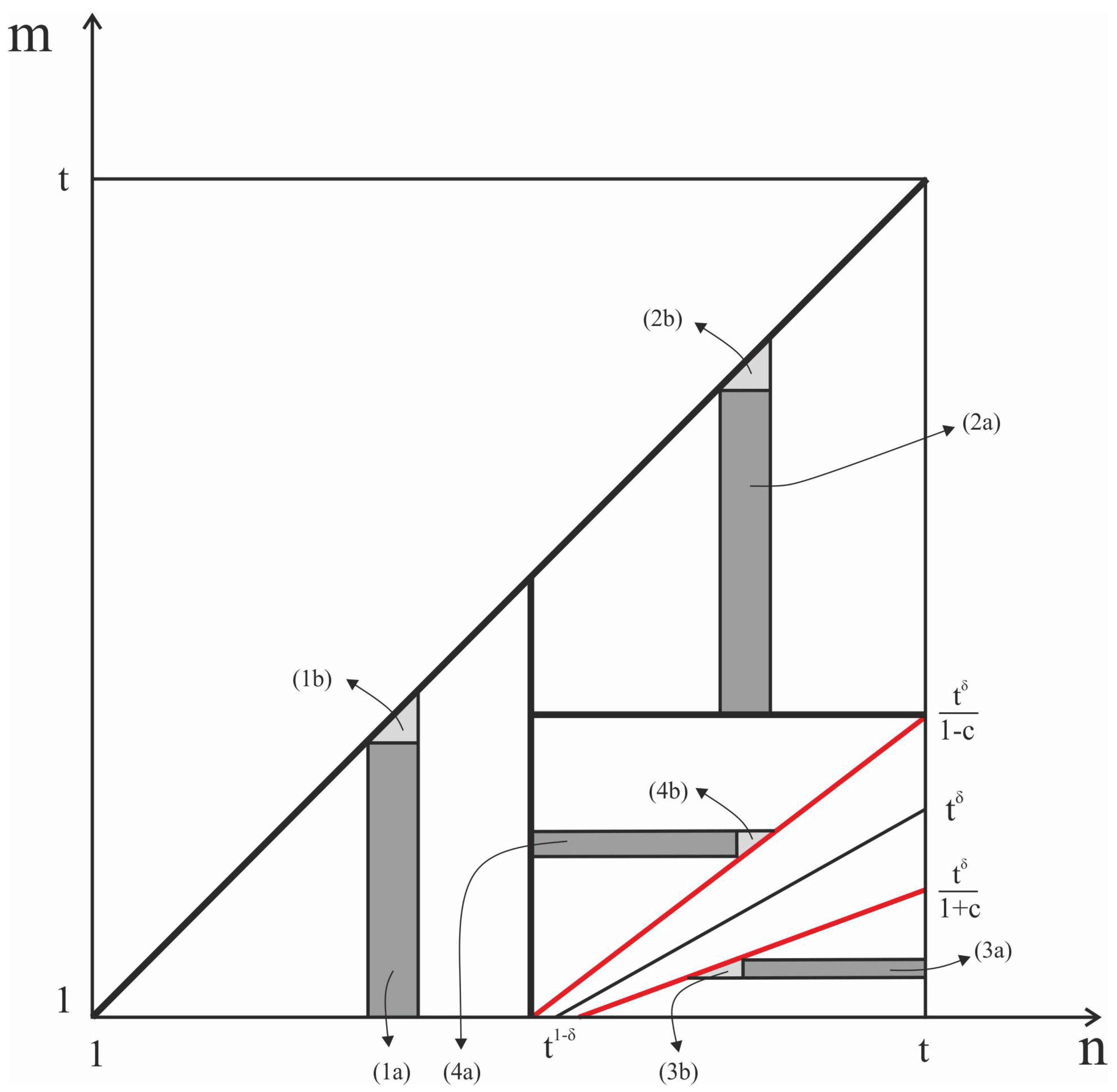
• For $1<M<\frac{1}{2}{t}^{1-\delta }$, two subregions:

  (1a)

  $m<M$ and $M<n<2M$.

  (1b)

  $M<m<n<2M$.

• For $\frac{1}{2}{t}^{1-\delta }<M<\frac{1}{2}t$, two subregions:

  (2a)

  $t^{\delta }<m<M$ and $M<n<2M$.

  (2b)

  $M<m<n<2M$.

• For $t^{1-\delta }<M<t$, two subregions:

  (3a)

  $M<m{t}^{1-\delta }<2M$ and $t^{1-\delta }<n<M$.

  (3b)

  $M<n<m{t}^{1-\delta }<2M$.

• For $t^{1-\delta }<M<t$, two subregions:

  (4a)

  $M<m{t}^{1-\delta }<2M$ and $2M<n<t$.

  (4b)

  $M<m{t}^{1-\delta }<n<2M$.

The first subregion of each of the above regions, namely (1a), (2a), (3a) and (4a), are of rectangular shape, see Figure 1. The corresponding sums are treated similarly to the $U\left(M\right)$ sums in [10]. It is straightforward to modify the relevant techniques therein according to the discussion of the case $S_1^{\left(i\right)}$ and obtain the essential bound of the rhs of (44). In fact, observing that in these regions $\frac{1}{ln\left(\frac{m}{n}{t}^{1-\delta }\right)}=O\left(1\right)$, one obtains the estimate $O\left(t^{\frac{1}{3}-\frac{\delta }{2}}{(lnt)}^2\right),t\to \infty$.

The subregions (1b) and (2b) are of triangular shape, see Figure 1, thus the corresponding sums are treated similarly to the $T\left(M\right)$ sums in [10]. The sums in these regions are treated in [10], via Lemma 3.5. It is straightforward to modify accordingly this approach and obtain the same bound as the rhs of (44).

The subregions (3b) and (4b) are also of triangular shape, see Figure 1. In order to analyse these sums we have to modify the approach of estimating the sums $T\left(M\right)$ in [10]. It is straightforward to modify the analysis of the oscillatory part of the sum, namely the part which uses the Lemmas 3.1–3.3 therein. For the analogue of the partial summation we need to use Lemma 2 instead of Lemma 3.5 in [10]. Then, we obtain the essential bound of the rhs of (44). In fact, observing that in these regions $\frac{1}{ln\left(\frac{m}{n}{t}^{1-\delta }\right)}=O\left(1\right)$, one obtains the estimate $O\left(t^{\frac{1}{3}-\frac{\delta }{2}}{(lnt)}^2\right),t\to \infty$.

4.4. An Alternative Way to Estimate $S_2^{\left(i\right)}$

It is possible to estimate $S_2^{\left(i\right)}$ using a different and less technical approach. Let us use the notation $D_2=\left\{(n,m)\in [1,t]\times [1,t],m<n\right\}$. Then, we rewrite

$$S_2^{\left(i\right)}=\frac{1}{t^{\frac{\delta }{2}}}\underset{(n,m)\in D_r}{\sum \sum }\frac{1}{n^{s+i{t}^{\delta }}}\frac{1}{m^{\overline{s}-i{t}^{\delta }}}\frac{1}{ln\left(\frac{m}{n}{t}^{1-\delta }\right)},$$

(47)

as

$$S_2^{\left(i\right)}=\frac{1}{t^{\frac{\delta }{2}}}\underset{(n,m)\in D_2}{\sum \sum }\frac{1}{n^{s+i{t}^{\delta }}}\frac{1}{m^{\overline{s}-i{t}^{\delta }}}F(n,m)-\frac{1}{t^{\frac{\delta }{2}}}\underset{(n,m)\in D_2\backslash D_r}{\sum \sum }\frac{1}{n^{s+i{t}^{\delta }}}\frac{1}{m^{\overline{s}-i{t}^{\delta }}}H(n,m),$$

(48)

where the functions F and H are $C^2$ and are defined as follows

$$F(x,y)=\left\{\begin{array}{cc}\frac{1}{ln\left(\frac{y}{x}{t}^{1-\delta }\right)},\hfill & (x,y)\in D_r,\hfill \\ H(x,y),\hfill & (x,y)\in D_2\backslash D_r,\hfill \end{array}\right.$$

(49)

with $D_r$ defined by the conditions (45). Furthermore, the function $P(x,y):D_2\to \mathbb{R}$, which is defined by $P(x,y):={\displaystyle \frac{F(x,y)}{x^{1/2}{y}^{1/2}}}$, belongs to $C^2$ and has the following properties:

$$\begin{array}{c}\hfill P(x,y)=O\left(\frac{1}{x^{1/2}{y}^{1/2}}\right),P_x(x,y)=O\left(\frac{1}{x^{3/2}{y}^{1/2}}\right),\\ \hfill P_y(x,y)=O\left(\frac{1}{x^{1/2}{y}^{3/2}}\right),P_{xy}(x,y)=O\left(\frac{1}{x^{3/2}{y}^{3/2}}\right).\end{array}$$

(50)

From (49) the set where we have to assure that $P(x,y)\in C^2\left(D_2\right)$ is given by the constraint $\frac{y}{x}{t}^{1-\delta }=1\pm c$, for some sufficiently small positive constant c. Hence, it is sufficient to determine the function $H(x,y)=d\left(\frac{y}{x}{t}^{1-\delta }\right),$ with the following six properties:

$$\begin{array}{c}\hfill d(1\pm c)={\displaystyle \frac{1}{ln(1\pm c)}},d^{\prime }(1\pm c)={\displaystyle \frac{1}{{\left[ln(1\pm c)\right]}^2(1\pm c)}},\\ \hfill d^{″}(1\pm c)={\displaystyle \frac{2+ln(1\pm c)}{{\left[ln(1\pm c)\right]}^3{(1\pm c)}^2}},\end{array}$$

(51)

for some fixed and sufficiently small $c>0$.

Furthermore, the conditions (50) are satisfied if the functions $d\left(r\right),d^{\prime }\left(r\right),d^{″}\left(r\right)$ are bounded in the interval $r\in (1-c,1+c)$.

Thus, it is sufficient for $d\left(r\right)$ to be a fifth order polynomial which satisfies the conditions (51).

Now, the sum $S_2^{\left(i\right)}$ has the appropriate form, so it can be analysed through the following two arguments:

• The first term of the rhs of (48) can be analysed in the same way as the sum $S_1^{\left(i\right)}$, with the only difference that in the current analysis we find it more convenient to employ the simpler version of partial summation technique described in Lemma A1.
• The second term of the rhs of (48) can be embedded in the analysis of the sum $S^{\left(ii\right)}$. In this case it is more convenient to employ a combination of partial summation techniques, as they are described in Lemmas 2 and A1, respectively.

The resulting estimate remains invariant.

5. Conclusions

The main result of this paper is the derivation of the Volterra-type linear integral Equation (8). In order to derive this equation starting from (1.6) of [9] it is necessary to:

(i)

replace $I_4$ by ${\tilde{I}}_4$ defined by (22).

(ii)

replace $S_4^P$ by (6).

(iii)

replace $S_4^{SD}$ by (7).

The derivation of (i) is based on replacing in the definition of $I_4$, the term ${\left|\zeta \left(s\right)\right|}^2$ by its leading asymptotics. The proof that the error term is indeed small is presented in [11].

The derivation of (ii) is given in Section 3.

The derivation of (iii) is given in Section 4 under the assumption that the function $E_4^{SD}$ appearing in $S_4^{SD}$ is given by Equations (36)–(38); the latter proof is given in [11].

The importance of the derivation of (8) is a consequence of the following considerations: taking into account that the variable $\rho$ appearing in the $\mathsf{\Gamma }$ functions in the integral of (8) satisfies $\rho \ge t^{{\delta }_2}$ and $t-\rho \ge t^{1/3}$, it follows that these $\mathsf{\Gamma }$ functions can be simplified as $t\to \infty$. Indeed, Equations (4.4), (5.7) and (5.8) on [9] yield

$$\begin{array}{cc}\frac{\mathsf{\Gamma }(it-i\rho )}{\mathsf{\Gamma }(1/2+it)}\mathsf{\Gamma }(1/2+i\rho )=\sqrt{\frac{2\pi }{t}}{e}^{-\frac{i\pi }{4}}\frac{1}{{\left(1-\frac{\rho }{t}\right)}^{1/2}}{e}^{it\left[\left(1-\frac{\rho }{t}\right)ln\left(1-\frac{\rho }{t}\right)+\frac{\rho }{t}ln\left(\frac{\rho }{t}\right)\right]}\hfill & \\ & \hfill \times \left[1+O\left(t^{-{\delta }_{23}}\right)\right],t\to \infty ,\end{array}$$

with ${\delta }_{23}=min\{{\delta }_2,{\delta }_3\}$.

Hence, for the specific choice of ${\delta }_2={\delta }_3=\frac{1}{3}$, replacing in Equation (8) the combination of the Gamma functions by the rhs of the above equation, we find

$$\begin{array}{cc}\hfill {\left|\zeta \left(\frac{1}{2}+it\right)\right|}^2=\sqrt{\frac{2}{\pi }}{\int }_{t^{1/3}}^{t-t^{1/3}}& \Re \left\{\frac{e^{-\frac{i\pi }{4}}}{{\left(t-\rho \right)}^{1/2}}{e}^{it\left[\left(1-\frac{\rho }{t}\right)ln\left(1-\frac{\rho }{t}\right)+\frac{\rho }{t}ln\left(\frac{\rho }{t}\right)\right]}\right\}{\left|\zeta \left(\frac{1}{2}+i\rho \right)\right|}^{2}d\rho \hfill \\ & \times \left[1+O\left(t^{-1/3}\right)\right]+O\left(t^{\frac{1}{6}}{(lnt)}^2\right),t\to \infty ,\hfill \end{array}$$

(52)

It is straightforward to show that the ansatz ${\left|\zeta \left(1/2+it\right)\right|}^2=O\left(t^{1/6}{(lnt)}^2\right)$ provides a solution of (52). The rigorous proof that the above ansatz provides the unique solution of the linear Volterra integral equation will be presented in [11]. This estimate implies that $\zeta \left(1/2+it\right)=O\left(t^{1/12}lnt\right)$, which is a dramatic improvement of the current best estimate of the large t behaviour of $\zeta \left(1/2+it\right)$.

References

- Weyl, H. Ueber die Gleichverteilung von Zahlen mod. Eins. Math. Ann. 1916, 77, 313–352. [Google Scholar] [CrossRef]
- Hardy, G.H.; Littlewood, J.E. Contributions to the theory of the Riemann zeta-function and the theory of the distribution of primes. Acta Math. 1916, 41, 119–196. [Google Scholar] [CrossRef]
- Vinogradov, I.M. A new method of estimation of trigonometrical sums. Mat. Sbornik 1936, 43, 175–188. [Google Scholar]
- Bourgain, J. Decoupling, exponential sums and the Riemann zeta function. J. Am. Math. Soc. 2017, 30, 205–224. [Google Scholar] [CrossRef]
- Siegel, C.L. Über Riemanns Nachlaßzur analytischen Zahlentheorie. In Quellen Studien zur Geschichte der Mathematik Astronomie und Physik Abteilung B: Studien 2: 4580, 1932; Springer: Berlin, Germany, 1966; Volume 1. [Google Scholar]
- Fokas, A.S.; Lenells, J. On the asymptotics to all orders of the Riemann Zeta function and of a two-parameter generalization of the Riemann Zeta function. arXiv 2012, to appear. arXiv:1201.2633. [Google Scholar]
- Fernandez, A.; Fokas, A.S. Asymptotics to all orders of the Hurwitz zeta function. J. Math. Anal. Appl. 2018, 465, 423–458. [Google Scholar] [CrossRef]
- Kalimeris, K.; Fokas, A.S. Explicit asymptotics for certain single and double exponential sums. Proc. R. Soc. Edinb. A Math. 2017, 1–26. [Google Scholar] [CrossRef]
- Fokas, A.S. A novel approach to the Lindelöf hypothesis. arXiv 2019, to appear. arXiv:1708.06607. [Google Scholar]
- Kiuci, I.; Tanigawa, Y. Bounds for double zeta functions. Annali della Scuola Normale Superiore di Pisa-Classe di Scienze 2006, 5, 445–464. [Google Scholar]
- Fokas, A.S.; Kalimeris, K.; Lenells, J. A Novel Integral Equation for the Riemann Zeta Function and a Significant Improvement of the Current Large t Estimate. 2019. in preparation. [Google Scholar]
- Krätzel, E. Lattice Points; Springer: Berlin, Germany, 1989. [Google Scholar]
- Titchmarsch, E.C. The Theory of the Riemann Zeta-Function, 2nd ed.; Oxford University Press: Oxford, UK, 1987. [Google Scholar]
- Titchmarsch, E.C. On Epstein’s Zeta-function. Proc. Lond. Math. Soc. 1934, 2, 485–500. [Google Scholar] [CrossRef]
- Ishikawa, H.; Matsumoto, K. On the estimation of the order of Euler-Zagier multiple zeta-functions. Ill. J. Math. 2003, 47, 1151–1166. [Google Scholar] [CrossRef]
© 2019 by the authors. Licensee MDPI, Basel, Switzerland. This article is an open access article distributed under the terms and conditions of the Creative Commons Attribution (CC BY) license (http://creativecommons.org/licenses/by/4.0/).
Share and Cite
Kalimeris, K.; Fokas, A.S. A Novel Integral Equation for the Riemann Zeta Function and Large t-Asymptotics. Mathematics 2019, 7, 650. https://doi.org/10.3390/math7070650
Kalimeris K, Fokas AS. A Novel Integral Equation for the Riemann Zeta Function and Large t-Asymptotics. Mathematics. 2019; 7(7):650. https://doi.org/10.3390/math7070650
Chicago/Turabian StyleKalimeris, Konstantinos, and Athanassios S. Fokas. 2019. "A Novel Integral Equation for the Riemann Zeta Function and Large t-Asymptotics" Mathematics 7, no. 7: 650. https://doi.org/10.3390/math7070650
APA StyleKalimeris, K., & Fokas, A. S. (2019). A Novel Integral Equation for the Riemann Zeta Function and Large t-Asymptotics. Mathematics, 7(7), 650. https://doi.org/10.3390/math7070650