Logarithmic Aggregation Operators of Picture Fuzzy Numbers for Multi-Attribute Decision Making Problems

Abstract

The objective of this study was to create a logarithmic decision-making approach to deal with uncertainty in the form of a picture fuzzy set. Firstly, we define the logarithmic picture fuzzy number and define the basic operations. As a generalization of the sets, the picture fuzzy set provides a more profitable method to express the uncertainties in the data to deal with decision making problems. Picture fuzzy aggregation operators have a vital role in fuzzy decision-making problems. In this study, we propose a series of logarithmic aggregation operators: logarithmic picture fuzzy weighted averaging/geometric and logarithmic picture fuzzy ordered weighted averaging/geometric aggregation operators and characterized their desirable properties. Finally, a novel algorithm technique was developed to solve multi-attribute decision making (MADM) problems with picture fuzzy information. To show the superiority and the validity of the proposed aggregation operations, we compared it with the existing method, and concluded from the comparison and sensitivity analysis that our proposed technique is more effective and reliable.

1. Introduction

Multiple attribute decision making (MADM) is a process for selecting the optimal alternative from a set of given alternatives according to some attributes. Due to the complexity of the socio-economic environment and decision makers’ insufficient knowledge and judgment, it is difficult for decision makers to provide accurate information about alternatives. For this, Atanassov [1] proposed the intuitionistic fuzzy set (IFS). IFS is an extension of fuzzy set (FS) [2], which is characterized by a positive membership degree and a negative membership degree, satisfying the condition that the sum of these two degrees is equal to or less than one; therefore, IFS is a useful tool in processing fuzzy and uncertainty information.

IFS has been practically applied in many fields, such as clustering analysis [3], decision making (DM) problems [4], medical diagnosis [5], and pattern recognition [6]. Many researchers have contributed to IFS. Chen et al. [7] presented a transformation method of intuitionistic fuzzy numbers (IFNs) and interval valued intuitionistic fuzzy (IVIF) numbers to aggregation operations to solve DM problems. Garg [8] introduce a robust improved geometric aggregation operation. Huang [9] introduced the intuitionistic fuzzy Hamacher aggregation operations and discussed their applications in decision making problems.

To aggregate the intuitionistic fuzzy information and make decisions, many intuitionistic fuzzy aggregation operators have been proposed for aggregating different alternatives [10,11]. However, in some special conditions, the sum of the positive membership degree and the negative membership degree provided by the decision maker may be greater than one. For instance, if a decision maker determines the positive membership as 0.3 and the negative membership degree may be 0.9, $0.3+0.9=1.2>1$. This situation cannot be handled by IFS. To overcome this problem, Yager [12,13] developed the concept of the Pythagorean fuzzy set (PyFS), which is also characterized by the positive membership degree and the negative membership degree, but the square sum of these two degrees is equal to or less than one. Corresponding to the above considered example, ${0.3}^2+{0.9}^2=0.9<1$. PyFS can solve many problems that IFS cannot. In other words, PyFS is a generalization of IFS; therefore, PyFS is more capable than IFS of modeling the imprecise and imperfect information in practical MADM problems. Since PyFS’s introduction, numerous aggregation operators have been proposed for aggregating Pythagorean fuzzy information [14,15].

In real life, some problems cannot be symbolized in IFS and PyFS. For example, for a voting system, human opinions include many answers of such types: yes, no, abstain, and refusal. Therefore, Cuong [16] introduced the core idea of the picture fuzzy set (PFS). PFS is an extension of IFS and PyFS. In the concept of the PFS, Cuong added the neutral term along with the positive membership and negative membership degrees and the sum of their membership degrees is equal to or less than one. Many researchers have attempted to contribute to the application of PFS. In 2014, Phong et al. [17] developed some composition of picture fuzzy relations. Singh [18] developed correlation coefficients for PFS and discussed their applications in decision making problems. In 2015, Cuong et al. [19] introduced the core idea about some fuzzy logic operations for picture fuzzy numbers. Thong et al. [20] developed a policy for multi-variable fuzzy forecasting using picture fuzzy (PF) clustering and a PF rules interpolation system. Son [21] presented the generalized picture distance measure and discussed its application. Wei [22] introduced PF cross-entropy and discussed its application in MADM problems. Ashraf et al. [23] proposed geometric aggregation operators and the Technique for Order of Preference by Similarity to Ideal Solution (TOPSIS) approach to deal with the uncertainty in decision making problems in the form of picture fuzzy sets. Garg [24] proposed some aggregation operators for picture fuzzy information and discussed their application in decision making problems. In 2017, Wei [25] introduced the PF aggregation operator based on t-norm and t-conorm and provided some discussion on its applications in decision making. In 2019, Zeng et al. [26] proposed the exponential Jensen picture fuzzy divergence measure and discussed its applications in multi-criteria decision making (MCDM).

Many aggregation operators have been developed based on the algebraic t-norm and t-conorm to deal with the aggregate uncertainty in the form of picture fuzzy sets. Logarithmic operational rules are important mathematical operations that conveniently use to aggregate uncertain and inaccurate data. Motivated by these ideas, we developed a picture fuzzy MCDM method based on the logarithmic aggregation operators and the logarithmic operations of PFSs to handle picture fuzzy MADM within PFSs.

The contributions of our method are as follows:

(1)

We developed some novel logarithmic operations for picture fuzzy sets, which can overcome the weaknesses of algebraic operations and capture the relationship between various PFSs.

(2)

We extended logarithmic operators to logarithmic picture fuzzy operators: logarithmic picture fuzzy weighted averaging (log-PFWA), logarithmic picture fuzzy ordered weighted averaging (log-PFOWA), logarithmic picture fuzzy weighted geometric (log-PFWG), and logarithmic picture fuzzy ordered weighted geometric (log-PFOWG) aggregation operators for picture fuzzy information, which can overcome the algebraic operators’ drawbacks.

(3)

We developed an algorithm to deal with multi-attribute decision making problems using picture fuzzy information.

(4)

To show the effectiveness and reliability of the proposed picture fuzzy logarithmic aggregation operators, we applied the proposed operator to a circulation center evaluation problem.

(5)

The results indicate that the proposed technique is more effective and provides a more accurate output compared to existing methods.

The remainder of this paper is organized as follows: Some basic knowledge related to IFS, PyFS, PFS, score, and accuracy function are defined in Section 2. In Section 3, we discuss the logarithmic operation laws and the properties of picture fuzzy numbers (PFNs), as well as logarithmic picture fuzzy averaging/geometric aggregation operators. In Section 4, we address the MADM problem, using logarithmic picture fuzzy aggregation operators. A descriptive example is outlined in Section 5; Section 5.1 provides a comparative analysis of the existing aggregation operators with the novel logarithmic aggregation operators defined in this study, and the conclusion of this study is draw in Section 6.

2. Background

The concepts and basic operations of existing extensions of fuzzy sets are recalled in this section, and they were the foundation of this study.

Definition 1.

[1] Let a fixed set $\mathrm{A}\ne \varphi$. Then, the set

$$J=\langle {\beta }_J\left(\dot{a}\right),{\pounds }_J\left(\dot{a}\right)|\dot{a}\in \mathrm{A}\rangle ,$$

is an IFS, where ${\beta }_J\left(\dot{a}\right),{\pounds }_J\left(\dot{a}\right)\in \left[0,1\right]$ are the positive and negative membership degrees of the element $\dot{a}\in \mathrm{A}$ in J, respectively. ${\beta }_J\left(\dot{a}\right),{\pounds }_J\left(\dot{a}\right)$ satisfy the condition for all $\dot{a}\in \mathrm{A},$

$$0\le {\beta }_J\left(\dot{a}\right)+{\pounds }_J\left(\dot{a}\right)\le 1.$$

Definition 2.

[16] Let a fixed set $\mathrm{A}\ne \varphi$. Then, the set

$$J=\langle {\beta }_J\left(\dot{a}\right),{\gamma }_J\left(\dot{a}\right),{\pounds }_J\left(\dot{a}\right)|\dot{a}\in \mathrm{A}\rangle ,$$

is said to be PFS, where ${\beta }_J\left(\dot{a}\right),{\gamma }_J\left(\dot{a}\right),{\pounds }_J\left(\dot{a}\right)\in \left[0,1\right]$ are the positive, neutral and negative membership degrees of the element $\dot{a}\in \mathrm{A}$ in $J$, respectively. ${\beta }_J\left(\dot{a}\right),{\gamma }_J\left(\dot{a}\right),{\pounds }_J\left(\dot{a}\right)$ satisfy the condition for all $\dot{a}\in \mathrm{A},$

$$0\le {\beta }_J\left(\dot{a}\right)+{\gamma }_J\left(\dot{a}\right)+{\pounds }_J\left(\dot{a}\right)\le 1.$$

For all $\dot{a}\in \mathrm{A},$ the refusal degree is ${\Theta }_J=1-\left({\beta }_J\left(\dot{a}\right)+{\gamma }_J\left(\dot{a}\right)+{\pounds }_J\left(\dot{a}\right)\right)$.

Definition 3.

[23] Let $J=\left({\beta }_J\left(\dot{a}\right),{\gamma }_J\left(\dot{a}\right),{\pounds }_J\left(\dot{a}\right)\right)$, $J_1=\left({\beta }_{J_1}\left(\dot{a}\right),{\gamma }_{J_1}\left(\dot{a}\right),{\pounds }_{J_1}\left(\dot{a}\right)\right)$ and $J_2=\left({\beta }_{J_2}\left(\dot{a}\right),{\gamma }_{J_2}\left(\dot{a}\right),{\pounds }_{J_2}\left(\dot{a}\right)\right)$ be any three PFNs, then:

1. 

$J^c=\left\{{\pounds }_J\left(\dot{a}\right),{\gamma }_J\left(\dot{a}\right),{\beta }_J\left(\dot{a}\right)\right\}$

2. 

$J_1\wedge J_2=\left\{\min \left({\beta }_{J_1}\left(\dot{a}\right),{\beta }_{J_2}\left(\dot{a}\right)\right),\max \left({\gamma }_{J_1}\left(\dot{a}\right),{\gamma }_{J_2}\left(\dot{a}\right)\right),\max \left({\pounds }_{J_1}\left(\dot{a}\right),{\pounds }_{J_2}\left(\dot{a}\right)\right)\right\}$

3. 

$J_1\vee J_2=\left\{\max \left({\beta }_{J_1}\left(\dot{a}\right),{\beta }_{J_2}\left(\dot{a}\right)\right),\min \left({\gamma }_{J_1}\left(\dot{a}\right),{\gamma }_{J_2}\left(\dot{a}\right)\right),\min \left({\pounds }_{J_1}\left(\dot{a}\right),{\pounds }_{J_2}\left(\dot{a}\right)\right)\right\}$

4. 

$J_1\oplus J_2=\left\{{\beta }_{J_1}\left(\dot{a}\right)+{\beta }_{J_2}\left(\dot{a}\right)-{\beta }_{J_1}\left(\dot{a}\right).{\beta }_{J_2}\left(\dot{a}\right),{\gamma }_{J_1}\left(\dot{a}\right).{\gamma }_{J_2}\left(\dot{a}\right),{\pounds }_{J_1}\left(\dot{a}\right).{\pounds }_{J_2}\left(\dot{a}\right)\right\}$

5. 

$J_1\otimes J_2=\left\{\begin{array}{c}{\beta }_{J_1}\left(\dot{a}\right).{\beta }_{J_2}\left(\dot{a}\right),{\gamma }_{J_1}\left(\dot{a}\right)+{\gamma }_{I_2}\left(\dot{a}\right)-{\gamma }_{J_1}\left(\dot{a}\right).{\gamma }_{J_2}\left(\dot{a}\right),\\ {\pounds }_{J_1}\left(\dot{a}\right)+{\pounds }_{J_2}\left(\dot{a}\right)-{\pounds }_{J_1}\left(\dot{a}\right).{\pounds }_{J_2}\left(\dot{a}\right)\end{array}\right\}$

6. 

$\upsilon .J=\left\{1-{\left(1-{\beta }_J\right)}^{\upsilon },\left({\gamma }_J\right){}^{\upsilon },\left({\pounds }_J\right){}^{\upsilon }\right\}$

7. 

$J^{\upsilon }=\left\{\left({\beta }_J\right){}^{\upsilon },1-{\left(1-{\gamma }_J\right)}^{\upsilon },1-{\left(1-{\pounds }_J\right)}^{\upsilon }\right\}$

Definition 4.

[23] Let $J=\langle {\beta }_J\left(\dot{a}\right),{\gamma }_J\left(\dot{a}\right),{\pounds }_J\left(\dot{a}\right)|\dot{a}\in \mathrm{A}\rangle$ be a PFN. The score function of $J$ is defined as:

$$S\left(J\right)={\beta }_J\left(\dot{a}\right)-{\gamma }_J\left(\dot{a}\right)-{\pounds }_J\left(\dot{a}\right),S\left(J\right)\in \left[-1,1\right].$$

The accuracy function of $J$ is defined as:

$$H\left(J\right)={\beta }_J\left(\dot{a}\right)+{\gamma }_J\left(\dot{a}\right)+{\pounds }_J\left(\dot{a}\right),H\left(J\right)\in \left[0,1\right].$$

Definition 5.

[23] Let $J_1=\left({\beta }_{J_1}\left(\dot{a}\right),{\gamma }_{J_1}\left(\dot{a}\right),{\pounds }_{J_1}\left(\dot{a}\right)\right)$ and $J_2=\left({\beta }_{J_2}\left(\dot{a}\right),{\gamma }_{J_2}\left(\dot{a}\right),{\pounds }_{J_2}\left(\dot{a}\right)\right)$ be two PFNs. Then, the comparison rules are defined as:

(1) 

If $S\left(J_1\right)>S\left(J_2\right),$ then $J_1>J_2$

(2) 

If $S\left(J_1\right)=S\left(J_2\right)$ and $H\left(J_1\right)>H\left(J_2\right),$ then $J_1>J_2$

(3) 

If $S\left(J_1\right)=S\left(J_2\right)$ and $H\left(J_1\right)=H\left(J_2\right),$ then $J_1=J_2$

3. Picture Fuzzy Logarithmic Aggregation Operators

In this section, we develop some novel logarithmic operational laws for picture fuzzy numbers and discuss their properties. The main purpose of this section is to propose novel logarithmic aggregation operators based on picture fuzzy information.

Note that $Lo{g}_{\tau }0$ is meaningless in the real number system and $Lo{g}_{\tau }1$ is not well defined. Therefore, we assume that $J\ne 0,$ where $J$ is a picture fuzzy number (PFN). Also, the base of log $\tau \ne 1$, $\tau$ is in the open interval (0, 1) and always a positive real number.

Definition 6.

Let $\mathrm{A}$ be non-empty fixed set and $J=\langle {\beta }_J\left(\dot{a}\right),{\gamma }_J\left(\dot{a}\right),{\pounds }_J\left(\dot{a}\right)|\dot{a}\in \mathrm{A}\rangle$ be a PFS. Then, the logarithmic picture fuzzy number is defined as:

$$Lo{g}_{\tau }J=\left\{\langle 1-Lo{g}_{\tau }{\beta }_J\left(\dot{a}\right),Lo{g}_{\tau }(1-{\gamma }_J\left(\dot{a}\right)),Lo{g}_{\tau }(1-{\pounds }_J\left(\dot{a}\right))\rangle \right\},0<\tau \le \beta \le 1,\tau \ne 1.$$

where ${\beta }_J\left(\dot{a}\right),{\gamma }_J\left(\dot{a}\right),{\pounds }_J\left(\dot{a}\right)$ are the positive, neutral, and negative membership degrees of the element $\dot{a}\in \mathrm{A}$ in $J$, respectively, with condition that $0\le {\beta }_J\left(\dot{a}\right),{\gamma }_J\left(\dot{a}\right),{\pounds }_J\left(\dot{a}\right)\le 1.$ Then, the positive membership is defined as:

$$\left(1-Lo{g}_{\tau }{\beta }_J\left(\dot{a}\right)\right):\mathrm{A}\to [0,1], \mathrm{such} \mathrm{that} \left(1-Lo{g}_{\tau }{\beta }_J\left(\dot{a}\right)\right)\in [0,1], \forall \dot{a}\in \mathrm{A},$$

the neutral membership is defined as:

$$Lo{g}_{\tau }(1-{\gamma }_J\left(\dot{a}\right)):\mathrm{A}\to [0,1], \mathrm{such} \mathrm{that} Lo{g}_{\tau }(1-{\gamma }_J\left(\dot{a}\right))\in [0,1], \forall \dot{a}\in \mathrm{A},$$

the negative membership is defined as:

$$Lo{g}_{\tau }(1-{\pounds }_J\left(\dot{a}\right)):\mathrm{A}\to [0,1], \mathrm{such} \mathrm{that} Lo{g}_{\tau }(1-{\pounds }_J\left(\dot{a}\right))\in [0,1], \forall \dot{a}\in \mathrm{A},$$

and the refusal degree is defined as:

$$1-\left(\left(1-Lo{g}_{\tau }{\beta }_J\left(\dot{a}\right)\right)+Lo{g}_{\tau }(1-{\gamma }_J\left(\dot{a}\right)+Lo{g}_{\tau }(1-{\pounds }_J\left(\dot{a}\right)\right)\in [0,1]; \forall \dot{a}\in \mathrm{A}.$$

Definition 7.

Let $J=\left({\beta }_J\left(\dot{a}\right),{\gamma }_J\left(\dot{a}\right),{\pounds }_J\left(\dot{a}\right)\right)$, $J_1=\left({\beta }_{J_1}\left(\dot{a}\right),{\gamma }_{J_1}\left(\dot{a}\right),{\pounds }_{J_1}\left(\dot{a}\right)\right)$, and $J_2=\left({\beta }_{J_2}\left(\dot{a}\right),{\gamma }_{J_2}\left(\dot{a}\right),{\pounds }_{J_2}\left(\dot{a}\right)\right)$ be any three PFNs. Then, the logarithmic operations are defined as:

(1) 

${\log }_{\tau }{J}_1\oplus {\log }_{\tau }{J}_2=\left(1-{\log }_{\tau }{\beta }_1.{\log }_{\tau }{\beta }_2,{\log }_{\tau }(1-{\gamma }_1).{\log }_{\tau }(1-{\gamma }_2),{\log }_{\tau }(1-{\pounds }_1).{\log }_{\tau }(1-{\pounds }_2)\right)$

(2) 

${\log }_{\tau }{J}_1\otimes {\log }_{\tau }{J}_2=\left(\begin{array}{c}\left(1-{\log }_{\tau }{\beta }_1\right).\left(1-{\log }_{\tau }{\beta }_2\right),1-(1-{\log }_{\tau }(1-{\gamma }_1)).(1-{\log }_{\tau }(1-{\gamma }_2)),\\ 1-(1-{\log }_{\tau }(1-{\pounds }_1)).(1-{\log }_{\tau }(1-{\pounds }_2))\end{array}\right)$

(3) 

$\upsilon .{\log }_{\tau }J=\left(1-{\left({\log }_{\tau }\beta \right)}^{\upsilon },{({\log }_{\tau }(1-\gamma ))}^{\upsilon },{({\log }_{\tau }(1-\pounds ))}^{\upsilon }\right)$

(4) 

${\log }_{\tau }{J}^{\upsilon }=\left(1-{\log }_{\tau }\beta {)}^{\upsilon },1-{(1-{\log }_{\tau }(1-\gamma ))}^{\upsilon },1-{(1-{\log }_{\tau }(1-\pounds ))}^{\upsilon }\right)$

Theorem 1.

Let $J=\langle {\beta }_J\left(\dot{a}\right),{\gamma }_J\left(\dot{a}\right),{\pounds }_J\left(\dot{a}\right)|\dot{a}\in \mathrm{A}\rangle$ be PFNs. If $0<\tau \le \beta \le 1$, $\tau \ne 1,$ then

(1) 

${\tau }^{Lo{g}_{\tau }J}=J.$

(2) 

$Lo{g}_{\tau }{\tau }^J=J.$

Proof. 

(1) According to the Definitions 6 and 7, we have:

$$\begin{array}{ll}{\tau }^{Lo{g}_{\tau }J}& =\left({\tau }^{1-(1-Lo{g}_{\tau }\beta )},1-{\tau }^{Lo{g}_{\tau }(1-\gamma )},1-{\tau }^{Lo{g}_{\tau }(1-\pounds )}\right)\\ & =\left({\tau }^{Lo{g}_{\tau }\beta },1-(1-\gamma ),1-(1-\pounds )\right)\\ & =\left(\beta ,\gamma ,\pounds \right)=J\end{array}$$

(2) Similarly, we have:

$$\begin{array}{ll}Lo{g}_{\tau }{\tau }^J& =Lo{g}_{\tau }\left({\tau }^{(1-\beta )},1-{\tau }^{\gamma },1-{\tau }^{\pounds }\right)\\ & =\left(1-Lo{g}_{\tau }{\tau }^{1-\beta },Lo{g}_{\tau }\left(1-\left(1-{\tau }^{\gamma }\right)),Lo{g}_{\tau }(1-(1-{\tau }^{\pounds })\right)\right)\\ & =\left(\beta ,\gamma ,\pounds \right)=J\end{array}$$

 □

Theorem 2.

Let $J_1=\left({\beta }_{J_1}\left(\dot{a}\right),{\gamma }_{J_1}\left(\dot{a}\right),{\pounds }_{J_1}\left(\dot{a}\right)\right)$ and $J_2=\left({\beta }_{J_2}\left(\dot{a}\right),{\gamma }_{J_2}\left(\dot{a}\right),{\pounds }_{J_2}\left(\dot{a}\right)\right)$ be any two PFNs with $\min ({\beta }_1,{\beta }_2)\ge \tau >0,$ $\tau \ne 1.$ Then,

(1) 

$Lo{g}_{\tau }{J}_1\oplus Lo{g}_{\tau }{J}_2=Lo{g}_{\tau }{J}_2\oplus Lo{g}_{\tau }{J}_1$ and

(2) 

$Lo{g}_{\tau }{J}_1\otimes Lo{g}_{\tau }{J}_2=Lo{g}_{\tau }{J}_2\otimes Lo{g}_{\tau }{J}_1$.

Proof. 

(1) According to the Definitions 6 and 7, we have

$$\begin{array}{ll}{\log }_{\tau }{J}_1\oplus {\log }_{\tau }{J}_2& =\left(\begin{array}{c}1-{\log }_{\tau }{\beta }_1,{\log }_{\tau }(1-{\gamma }_1),\\ {\log }_{\tau }(1-{\pounds }_1)\end{array}\right)\oplus \left(\begin{array}{c}1-{\log }_{\tau }{\beta }_2,{\log }_{\tau }(1-{\gamma }_2),\\ {\log }_{\tau }(1-{\pounds }_2)\end{array}\right)\\ & =\left(\begin{array}{c}1-{\log }_{\tau }{\beta }_1.{\log }_{\tau }{\beta }_2,{\log }_{\tau }(1-{\gamma }_1).{\log }_{\tau }(1-{\gamma }_2),\\ {\log }_{\tau }(1-{\pounds }_1).{\log }_{\tau }(1-{\pounds }_2)\end{array}\right)\end{array}$$

$$\begin{array}{ll}{\log }_{\tau }{J}_2\oplus {\log }_{\tau }{J}_1& =\left(\begin{array}{c}1-{\log }_{\tau }{\beta }_2,{\log }_{\tau }(1-{\gamma }_2),\\ {\log }_{\tau }(1-{\pounds }_2)\end{array}\right)\oplus \left(\begin{array}{c}1-{\log }_{\tau }{\beta }_1,{\log }_{\tau }(1-{\gamma }_1),\\ {\log }_{\tau }(1-{\pounds }_1)\end{array}\right)\\ & =\left(\begin{array}{c}1-{\log }_{\tau }{\beta }_2.{\log }_{\tau }{\beta }_1,{\log }_{\tau }(1-{\gamma }_2).{\log }_{\tau }(1-{\gamma }_1),\\ {\log }_{\tau }(1-{\pounds }_2).{\log }_{\tau }(1-{\pounds }_1)\end{array}\right)\\ & =\left(\begin{array}{c}1-{\log }_{\tau }{\beta }_1.{\log }_{\tau }{\beta }_2,{\log }_{\tau }(1-{\gamma }_1).{\log }_{\tau }(1-{\gamma }_2),\\ {\log }_{\tau }(1-{\pounds }_1).{\log }_{\tau }(1-{\pounds }_2)\end{array}\right),\end{array}$$

Therefore, we have:

$${\log }_{\tau }{J}_1\oplus {\log }_{\tau }{J}_2={\log }_{\tau }{J}_2\oplus {\log }_{\tau }{J}_1.$$

(2) Similarly, we have:

$$\begin{array}{ll}{\log }_{\tau }{J}_1\otimes {\log }_{\tau }{J}_2& =\left(\begin{array}{c}1-{\log }_{\tau }{\beta }_1,{\log }_{\tau }(1-{\gamma }_1),\\ {\log }_{\tau }(1-{\pounds }_1)\end{array}\right)\otimes \left(\begin{array}{c}1-{\log }_{\tau }{\beta }_2,{\log }_{\tau }(1-{\gamma }_2),\\ {\log }_{\tau }(1-{\pounds }_2)\end{array}\right)\\ & =\left(\begin{array}{l}\left(1-{\log }_{\tau }{\beta }_1\right).\left(1-{\log }_{\tau }{\beta }_2\right),1-(1-{\log }_{\tau }(1-{\gamma }_1)).(1-{\log }_{\tau }(1-{\gamma }_2)),\\ 1-(1-{\log }_{\tau }(1-{\pounds }_1)).(1-{\log }_{\tau }(1-{\pounds }_2))\end{array}\right)\end{array} \mathrm{and}$$

$$\begin{array}{ll}{\log }_{\tau }{J}_2\otimes {\log }_{\tau }{J}_1& =\left(\begin{array}{c}1-{\log }_{\tau }{\beta }_2,{\log }_{\tau }(1-{\gamma }_2),\\ {\log }_{\tau }(1-{\pounds }_2)\end{array}\right)\otimes \left(\begin{array}{c}1-{\log }_{\tau }{\beta }_1,{\log }_{\tau }(1-{\gamma }_1),\\ {\log }_{\tau }(1-{\pounds }_1)\end{array}\right)\\ & =\left(\begin{array}{l}\left(1-{\log }_{\tau }{\beta }_2\right).\left(1-{\log }_{\tau }{\beta }_1\right),1-(1-{\log }_{\tau }(1-{\gamma }_2)).(1-{\log }_{\tau }(1-{\gamma }_1)),\\ 1-(1-{\log }_{\tau }(1-{\pounds }_2)).(1-{\log }_{\tau }(1-{\pounds }_1))\end{array}\right)\\ & =\left(\begin{array}{l}\left(1-{\log }_{\tau }{\beta }_1\right).\left(1-{\log }_{\tau }{\beta }_2\right),1-(1-{\log }_{\tau }(1-{\gamma }_1)).(1-{\log }_{\tau }(1-{\gamma }_2)),\\ 1-(1-{\log }_{\tau }(1-{\pounds }_1)).(1-{\log }_{\tau }(1-{\pounds }_2))\end{array}\right)\end{array}.$$

Therefore, we have:

$${\log }_{\tau }{J}_1\otimes {\log }_{\tau }{J}_2={\log }_{\tau }{J}_2\otimes {\log }_{\tau }{J}_1.$$

 □

3.1. Logarithmic Picture Fuzzy Averaging Aggregation Operators

In this subsection, we define some logarithmic aggregation operators: picture fuzzy logarithmic weighted averaging and picture fuzzy logarithmic order weighted averaging aggregation operators. We also discuss their properties in detail.

Definition 8.

Let $J_{ħ}=\langle {\beta }_{ħ},{\gamma }_{ħ},{\pounds }_{ħ}\rangle$ $\left(ħ=1,2,\cdots n\right)$ be any collection of PFNs with $0<{\tau }_{ħ}\le {\beta }_{ħ}\le 1$ and ${\tau }_{ħ}\ne 1$. Then, the mapping $Log-PFWA:{\Phi }^n\to \Phi$ is defined as:

$$Log-PFWA\left(J_1,\cdots ,J_n\right)=\underset{ħ=1}{\overset{n}{\oplus }}{\upsilon }_{ħ}.Lo{g}_{{\tau }_{ħ}}{J}_{ħ},.$$

The function Log-PFWA is known as the logarithmic PF weighted averaging operator, where $\upsilon ={\left({\upsilon }_1,{\upsilon }_2,\cdots ,{\upsilon }_n\right)}^T$, the weighed vectors, are Log-PFNs, such that ${\upsilon }_{ħ}\in \left[0,1\right]$ and ${\sum }_{ħ=1}^n{\upsilon }_{ħ}=1,$.

Theorem 3.

Let $J_{ħ}=\langle {\beta }_{ħ},{\gamma }_{ħ},{\pounds }_{ħ}\rangle \left(ħ=1,2,\cdots n\right)$ be any collection of PFNs with $0<{\tau }_{ħ}\le {\beta }_{ħ}\le 1$ and ${\tau }_{ħ}\ne 1$. Then, using Definitions 6 and 7, we have:

$$Log-PFWA\left(J_1,\cdots J_n\right)=\left(1-{\displaystyle \prod _{ħ=1}^n{\left({\log }_{{\tau }_{ħ}}{\beta }_{ħ}\right)}^{{\upsilon }_{ħ}}},{\displaystyle \prod _{ħ=1}^n{\left({\log }_{{\tau }_{ħ}}\left(1-{\gamma }_{ħ}\right)\right)}^{{\upsilon }_{ħ}}},{\displaystyle \prod _{ħ=1}^n{\left({\log }_{{\tau }_{ħ}}\left(1-{\pounds }_{ħ}\right)\right)}^{{\upsilon }_{ħ}}}\right).$$

where $\upsilon ={\left({\upsilon }_1,{\upsilon }_2,\cdots ,{\upsilon }_n\right)}^T$ are the weighted vectors, such that ${\upsilon }_{ħ}\in \left[0,1\right]$, ${\sum }_{ħ=1}^n{\upsilon }_{ħ}=1,$ and $\left(\forall ħ=1,2,\cdots n\right).$

Proof. 

Now, we proof using mathematical induction.

So, for $n=2,$ we have

$$Log-PFWA\left(J_1,J_2\right)={\upsilon }_1.{\log }_{{\tau }_1}{J}_1\oplus {\upsilon }_2.{\log }_{{\tau }_2}{J}_2,$$

where

$${\upsilon }_1.{\log }_{{\tau }_1}{J}_1=\left(1-{\left({\log }_{{\tau }_1}{\beta }_1\right)}^{{\upsilon }_1},{\left({\log }_{{\tau }_1}\left(1-{\gamma }_1\right)\right)}^{{\upsilon }_1},{\left({\log }_{{\tau }_1}\left(1-{\pounds }_1\right)\right)}^{{\upsilon }_1}\right)$$

and

$${\upsilon }_2.{\log }_{{\tau }_2}{J}_2=\left(1-{\left({\log }_{{\tau }_2}{\beta }_2\right)}^{{\upsilon }_2},{\left({\log }_{{\tau }_2}\left(1-{\gamma }_2\right)\right)}^{{\upsilon }_2},{\left({\log }_{{\tau }_2}\left(1-{\pounds }_2\right)\right)}^{{\upsilon }_2}\right)$$

$$Log-PFWA\left(J_1,J_2\right)=\left(\begin{array}{c}1-{\left({\log }_{{\tau }_1}{\beta }_1\right)}^{{\upsilon }_1},\\ {\left({\log }_{{\tau }_1}\left(1-{\gamma }_1\right)\right)}^{{\upsilon }_1},\\ {\left({\log }_{{\tau }_1}\left(1-{\pounds }_1\right)\right)}^{{\upsilon }_1}\end{array}\right)\oplus \left(\begin{array}{c}1-{\left({\log }_{{\tau }_2}{\beta }_2\right)}^{{\upsilon }_2},\\ {\left({\log }_{{\tau }_2}\left(1-{\gamma }_2\right)\right)}^{{\upsilon }_2},\\ {\left({\log }_{{\tau }_2}\left(1-{\pounds }_2\right)\right)}^{{\upsilon }_2}\end{array}\right).$$

Using Definition 7, we have

$$Log-PFWA\left(J_1,J_2\right)=\left(1-{\displaystyle \prod _{ħ=1}^2{\left({\log }_{{\tau }_{ħ}}{\beta }_{ħ}\right)}^{{\upsilon }_{ħ}}},{\displaystyle \prod _{ħ=1}^2{\left({\log }_{{\tau }_{ħ}}\left(1-{\gamma }_{ħ}\right)\right)}^{{\upsilon }_{ħ}}},{\displaystyle \prod _{ħ=1}^2{\left({\log }_{{\tau }_{ħ}}\left(1-{\pounds }_{ħ}\right)\right)}^{{\upsilon }_{ħ}}}\right).$$

Suppose that Theorem 3 is true for $n=k$:

$$Log-PFWA\left(J_1,\cdots J_k\right)=\left(1-{\displaystyle \prod _{ħ=1}^k{\left({\log }_{{\tau }_{ħ}}{\beta }_{ħ}\right)}^{{\upsilon }_{ħ}}},{\displaystyle \prod _{ħ=1}^k{\left({\log }_{{\tau }_{ħ}}\left(1-{\gamma }_{ħ}\right)\right)}^{{\upsilon }_{ħ}}},{\displaystyle \prod _{ħ=1}^k{\left({\log }_{{\tau }_{ħ}}\left(1-{\pounds }_{ħ}\right)\right)}^{{\upsilon }_{ħ}}}\right).$$

Now, we must prove that Theorem 3 is true for $n=k+1$:

$$\begin{array}{ll}Log-PFWA\left(J_1,J_2,\dots ,J_k,J_{k+1}\right)& ={\upsilon }_1.{\log }_{{\tau }_1}{J}_1\oplus {\upsilon }_2.{\log }_{{\tau }_2}{J}_2\oplus \cdots \oplus {\upsilon }_k.{\log }_{{\tau }_k}{J}_k\oplus {\upsilon }_{k+1}.{\log }_{{\tau }_{k+1}}{J}_{k+1}\\ & =\left(\begin{array}{l}1-{\displaystyle \prod _{ħ=1}^k{\left({\log }_{{\tau }_{ħ}}{\beta }_{ħ}\right)}^{{\upsilon }_{ħ}}},\\ {\displaystyle \prod _{ħ=1}^k{\left({\log }_{{\tau }_{ħ}}\left(1-{\gamma }_{ħ}\right)\right)}^{{\upsilon }_{ħ}}},\\ {\displaystyle \prod _{ħ=1}^k{\left({\log }_{{\tau }_{ħ}}\left(1-{\pounds }_{ħ}\right)\right)}^{{\upsilon }_{ħ}}}\end{array}\right)\oplus \left(\begin{array}{l}1-{\left({\log }_{{\tau }_{k+1}}{\beta }_{k+1}\right)}^{{\upsilon }_{k+1}},\\ {\left({\log }_{{\tau }_{k+1}}\left(1-{\gamma }_{k+1}\right)\right)}^{{\upsilon }_{k+1}},\\ {\left({\log }_{{\tau }_{k+1}}\left(1-{\pounds }_{k+1}\right)\right)}^{{\upsilon }_{k+1}}\end{array}\right)\end{array}$$

Using Definition 7, we have:

$$=\left(1-{\displaystyle \prod _{ħ=1}^{k+1}{\left({\log }_{{\tau }_{ħ}}{\beta }_{ħ}\right)}^{{\upsilon }_{ħ}}},{\displaystyle \prod _{ħ=1}^{k+1}{\left({\log }_{{\tau }_{ħ}}\left(1-{\gamma }_{ħ}\right)\right)}^{{\upsilon }_{ħ}}},{\displaystyle \prod _{ħ=1}^{k+1}{\left({\log }_{{\tau }_{ħ}}\left(1-{\pounds }_{ħ}\right)\right)}^{{\upsilon }_{ħ}}}\right).$$

Hence, the result holds for $n=k+1.$ Thus, the result is true for all n, i.e.:

$$Log-PFWA\left(J_1,\cdots J_n\right)=\left(1-{\displaystyle \prod _{ħ=1}^n{\left({\log }_{{\tau }_{ħ}}{\beta }_{ħ}\right)}^{{\upsilon }_{ħ}}},{\displaystyle \prod _{ħ=1}^n{\left({\log }_{{\tau }_{ħ}}\left(1-{\gamma }_{ħ}\right)\right)}^{{\upsilon }_{ħ}}},{\displaystyle \prod _{ħ=1}^n{\left({\log }_{{\tau }_{ħ}}\left(1-{\pounds }_{ħ}\right)\right)}^{{\upsilon }_{ħ}}}\right).$$

 □

Theorem 4.

(1) Idempotency: Let $J_{ħ}=\langle {\beta }_{ħ},{\gamma }_{ħ},{\pounds }_{ħ}\rangle \left(ħ=1,2,\cdots n\right)$ be any collection of PFNs and $J_{ħ}=J,$ with $\left(ħ=1,2,\cdots n\right)$. Then we have:

$$Log-PFWA\left(J_1,\cdots ,J_n\right)=Lo{g}_{\tau }J,$$

where ${\tau }_1={\tau }_2=\cdots ={\tau }_n=\tau .$

(2) Boundedness: Let $J_{ħ}=\langle {\beta }_{ħ},{\gamma }_{ħ},{\pounds }_{ħ}\rangle \left(ħ=1,2,\cdots n\right)$ be any collection of PFNs, and we have $J^{-}=\min \left(J_1,\cdots ,J_n\right)$ and $J^{+}=\max \left(J_1,J_2,\cdots ,J_n\right),$. Then:

$$J^{-}\le Log-PFWA\left(J_1,J_2,\cdots ,J_n\right)\le J^{+},$$

where ${\tau }_1={\tau }_2=\cdots ={\tau }_n=\tau .$

(3) Monotonicity: Let $J_{ħ}=\left({\beta }_{ħ},{\gamma }_{ħ},{\pounds }_{ħ}\right)$ and $J_{ħ}^{\ast }=\left({\beta }_{ħ}^{\ast },{\gamma }_{ħ}^{\ast },{\pounds }_{ħ}^{\ast }\right)$, where $\left(ħ=1,2,\cdots n\right)$ be a collection of PFNs. If ${\beta }_{ħ}\le {\beta }_{ħ}^{\ast },{\gamma }_{ħ}\ge {\gamma }_{ħ}^{\ast }$ and ${\pounds }_{ħ}\ge {\pounds }_{ħ}^{\ast },$ and $0<{\tau }_{ħ}\le \min \left({\beta }_{ħ},{\beta }_{ħ}^{\ast }\right)\le 1,$ holds for any $ħ,$ then:

$$Log-PFWA\left(J_1,\cdots ,J_n\right)\le Log-PFWA\left(J_1^{\ast },\cdots ,J_n^{\ast }\right).$$

Proof of Theorem 4 (1).

Since $J_{ħ}=\langle {\beta }_{ħ},{\gamma }_{ħ},{\pounds }_{ħ}\rangle \left(ħ=1,2,\cdots n\right)$ is any collection of PFNs, with $J_{ħ}=J$ $\left(ħ=1,2,\cdots n\right)$; then, using Theorem 3, we have:

$$\begin{array}{l}Log-PFWA\left(J_1,\cdots J_n\right)=\left(1-{\displaystyle \prod _{ħ=1}^n{\left({\log }_{{\tau }_{ħ}}{\beta }_{ħ}\right)}^{{\upsilon }_{ħ}}},{\displaystyle \prod _{ħ=1}^n{\left({\log }_{{\tau }_{ħ}}\left(1-{\gamma }_{ħ}\right)\right)}^{{\upsilon }_{ħ}}},{\displaystyle \prod _{ħ=1}^n{\left({\log }_{{\tau }_{ħ}}\left(1-{\pounds }_{ħ}\right)\right)}^{{\upsilon }_{ħ}}}\right).\\ =\left(1-{\displaystyle \prod _{ħ=1}^n{\left({\log }_{\tau }\beta \right)}^{{\upsilon }_{ħ}}},{\displaystyle \prod _{ħ=1}^n{\left({\log }_{\tau }\left(1-\gamma \right)\right)}^{{\upsilon }_{ħ}}},{\displaystyle \prod _{ħ=1}^n{\left({\log }_{\tau }\left(1-\pounds \right)\right)}^{{\upsilon }_{ħ}}}\right)\\ =\left(1-{\left({\log }_{\tau }\beta \right)}^{{\displaystyle \sum _{ħ=1}^n{\upsilon }_{ħ}}},{\left({\log }_{\tau }\left(1-\gamma \right)\right)}^{{\displaystyle \sum _{ħ=1}^n{\upsilon }_{ħ}}},{\left({\log }_{\tau }\left(1-\pounds \right)\right)}^{{\displaystyle \sum _{ħ=1}^n{\upsilon }_{ħ}}}\right)\\ =\left(1-\left({\log }_{\tau }\beta \right),{\log }_{\tau }\left(1-\gamma \right),{\log }_{\tau }\left(1-\pounds \right)\right)={\log }_{\tau }J\end{array}$$

 □

Proof of Theorem 4 (2).

$J_{ħ}=\langle {\beta }_{ħ},{\gamma }_{ħ},{\pounds }_{ħ}\rangle \left(ħ=1,2,\cdots n\right)$ is any collection of PFNs and $J_{ħ}^{-}=\min \left(J_1,\cdots ,J_n\right)=\left({\beta }^{-},{\gamma }^{-},{\pounds }^{-}\right)$, i.e., ${\beta }^{-}=\min \left({\beta }_{ħ}\right)$, ${\gamma }^{-}=\max \left({\gamma }_{ħ}\right)$, ${\pounds }^{-}=\max \left({\pounds }_{ħ}\right)$ and similarly $J_{ħ}^{+}=\max \left(J_1,J_2,\cdots ,J_n\right)=\left({\beta }^{+},{\gamma }^{+},{\pounds }^{+}\right)$ ${\beta }^{+}=\max \left({\beta }_{ħ}\right)$, ${\gamma }^{+}=\min \left({\gamma }_{ħ}\right)$, ${\pounds }^{+}=\min \left({\pounds }_{ħ}\right)$. Hence, we have:

$$\begin{array}{c}\underset{ħ}{\min }\left\{{\beta }_{ħ}\right\}\le {\beta }_{ħ}\le \underset{ħ}{\max }\left\{{\beta }_{ħ}\right\}\\ \underset{ħ}{\min }\left\{{\gamma }_{ħ}\right\}\le {\gamma }_{ħ}\le \underset{ħ}{\max }\left\{{\gamma }_{ħ}\right\}\\ \underset{ħ}{\min }\left\{{\pounds }_{ħ}\right\}\le {\pounds }_{ħ}\le \underset{ħ}{\max }\left\{{\pounds }_{ħ}\right\}.\end{array}$$

$$\begin{array}{ll}1-{\displaystyle \prod _{ħ=1}^n{\left({\log }_{\tau }{\beta }_{ħ}\right)}^{{\upsilon }_{ħ}}}& \ge 1-{\displaystyle \prod _{ħ=1}^n{\left({\log }_{\tau }\left(\underset{ħ}{\min }\left\{{\beta }_{ħ}\right\}\right)\right)}^{{\upsilon }_{ħ}}}\\ & =1-{\left({\log }_{\tau }\left(\underset{ħ}{\min }\left\{{\beta }_{ħ}\right\}\right)\right)}^{{\displaystyle \sum _{ħ=1}^n{\upsilon }_{ħ}}}\\ & =1-{\log }_{\tau }\left(\underset{ħ}{\min }\left\{{\beta }_{ħ}\right\}\right).\end{array}$$

$$\begin{array}{ll}1-{\displaystyle \prod _{ħ=1}^n{\left({\log }_{\tau }{\beta }_{ħ}\right)}^{{\upsilon }_{ħ}}}& \le 1-{\displaystyle \prod _{ħ=1}^n{\left({\log }_{\tau }\left(\underset{ħ}{\max }\left\{{\beta }_{ħ}\right\}\right)\right)}^{{\upsilon }_{ħ}}}\\ & =1-{\left({\log }_{\tau }\left(\underset{ħ}{\max }\left\{{\beta }_{ħ}\right\}\right)\right)}^{{\displaystyle \sum _{ħ=1}^n{\upsilon }_{ħ}}}\\ & =1-{\log }_{\tau }\left(\underset{ħ}{\max }\left\{{\beta }_{ħ}\right\}\right).\end{array}$$

$$\begin{array}{ll}{\displaystyle \prod _{ħ=1}^n{\left({\log }_{\tau }\left(1-{\gamma }_{ħ}\right)\right)}^{{\upsilon }_{ħ}}}& \ge {\displaystyle \prod _{ħ=1}^n{\left({\log }_{\tau }\left(1-\underset{ħ}{\min }\left\{{\gamma }_{ħ}\right\}\right)\right)}^{{\upsilon }_{ħ}}}\\ & ={\left({\log }_{\tau }\left(1-\underset{ħ}{\min }\left\{{\gamma }_{ħ}\right\}\right)\right)}^{{\displaystyle \sum _{ħ=1}^n{\upsilon }_{ħ}}}\\ & ={\log }_{\tau }\left(1-\underset{ħ}{\min }\left\{{\gamma }_{ħ}\right\}\right)\end{array}$$

$$\begin{array}{l}{\displaystyle \prod _{ħ=1}^n{\left({\log }_{\tau }\left(1-{\gamma }_{ħ}\right)\right)}^{{\upsilon }_{ħ}}}\le {\displaystyle \prod _{ħ=1}^n{\left({\log }_{\tau }\left(1-\underset{ħ}{\max }\left\{{\gamma }_{ħ}\right\}\right)\right)}^{{\upsilon }_{ħ}}}\\ ={\left({\log }_{\tau }\left(1-\underset{ħ}{\max }\left\{{\gamma }_{ħ}\right\}\right)\right)}^{{\displaystyle \sum _{ħ=1}^n{\upsilon }_{ħ}}}\\ ={\log }_{\tau }\left(1-\underset{ħ}{\max }\left\{{\gamma }_{ħ}\right\}\right)\end{array}$$

$$\begin{array}{ll}{\displaystyle \prod _{ħ=1}^n{\left({\log }_{\tau }\left(1-{\pounds }_{ħ}\right)\right)}^{{\upsilon }_{ħ}}}& \ge {\displaystyle \prod _{ħ=1}^n{\left({\log }_{\tau }\left(1-\underset{ħ}{\min }\left\{{\pounds }_{ħ}\right\}\right)\right)}^{{\upsilon }_{ħ}}}\\ & ={\left({\log }_{\tau }\left(1-\underset{ħ}{\min }\left\{{\pounds }_{ħ}\right\}\right)\right)}^{{\displaystyle \sum _{ħ=1}^n{\upsilon }_{ħ}}}\\ & ={\log }_{\tau }\left(1-\underset{ħ}{\min }\left\{{\pounds }_{ħ}\right\}\right)\end{array}$$

$$\begin{array}{l}{\displaystyle \prod _{ħ=1}^n{\left({\log }_{\tau }\left(1-{\pounds }_{ħ}\right)\right)}^{{\upsilon }_{ħ}}}\le {\displaystyle \prod _{ħ=1}^n{\left({\log }_{\tau }\left(1-\underset{ħ}{\max }\left({\pounds }_{ħ}\right)\right)\right)}^{{\upsilon }_{ħ}}}\\ ={\left({\log }_{\tau }\left(1-\underset{ħ}{\max }\left\{{\pounds }_{ħ}\right\}\right)\right)}^{{\displaystyle \sum _{ħ=1}^n{\upsilon }_{ħ}}}\\ ={\log }_{\tau }\left(1-\underset{ħ}{\max }\left\{{\pounds }_{ħ}\right\}\right)\end{array}$$

Therefore, we have

$$J^{-}\le PFWA\left(J_1,J_2,\cdots ,J_n\right)\le J^{+}.$$

 □

Proof of Theorem 4 (3).

Let

$$J=Log-PFWA\left(J_1,\cdots J_n\right)=\left(1-{\displaystyle \prod _{ħ=1}^n{\left({\log }_{{\tau }_{ħ}}{\beta }_{ħ}\right)}^{{\upsilon }_{ħ}}},{\displaystyle \prod _{ħ=1}^n{\left({\log }_{{\tau }_{ħ}}\left(1-{\gamma }_{ħ}\right)\right)}^{{\upsilon }_{ħ}}},{\displaystyle \prod _{ħ=1}^n{\left({\log }_{{\tau }_{ħ}}\left(1-{\pounds }_{ħ}\right)\right)}^{{\upsilon }_{ħ}}}\right).$$

and

$$J^{*}=Log-PFWA\left(J_1^{\ast },\cdots J_n^{\ast }\right)=\left(1-{\displaystyle \prod _{ħ=1}^n{\left({\log }_{{\tau }_{ħ}}{\beta }_{ħ}^{\ast }\right)}^{{\upsilon }_{ħ}}},{\displaystyle \prod _{ħ=1}^n{\left({\log }_{{\tau }_{ħ}}\left(1-{\gamma }_{ħ}^{\ast }\right)\right)}^{{\upsilon }_{ħ}}},{\displaystyle \prod _{ħ=1}^n{\left({\log }_{{\tau }_{ħ}}\left(1-{\pounds }_{ħ}^{\ast }\right)\right)}^{{\upsilon }_{ħ}}}\right).$$

However, if ${\beta }_{ħ}\le {\beta }_{ħ}^{\ast },$ ${\gamma }_{ħ}\ge {\gamma }_{ħ}^{\ast }$, and ${\pounds }_{ħ}\ge {\pounds }_{ħ}^{\ast },$ for any $ħ$, then:

$$1-{\displaystyle \prod _{ħ=1}^n{\left({\log }_{{\tau }_{ħ}}{\beta }_{ħ}\right)}^{{\upsilon }_{ħ}}}\le 1-{\displaystyle \prod _{ħ=1}^n{\left({\log }_{{\tau }_{ħ}}{\beta }_{ħ}^{\ast }\right)}^{{\upsilon }_{ħ}}}$$

$${\displaystyle \prod _{ħ=1}^n{\left({\log }_{{\tau }_{ħ}}\left(1-{\gamma }_{ħ}\right)\right)}^{{\upsilon }_{ħ}}}\ge {\displaystyle \prod _{ħ=1}^n{\left({\log }_{{\tau }_{ħ}}\left(1-{\gamma }_{ħ}^{\ast }\right)\right)}^{{\upsilon }_{ħ}}}$$

$${\displaystyle \prod _{ħ=1}^n{\left({\log }_{{\tau }_{ħ}}\left(1-{\pounds }_{ħ}\right)\right)}^{{\upsilon }_{ħ}}}\ge {\displaystyle \prod _{ħ=1}^n{\left({\log }_{{\tau }_{ħ}}\left(1-{\pounds }_{ħ}^{\ast }\right)\right)}^{{\upsilon }_{ħ}}}$$

Therefore, using the definition of the score function and the accuracy function, we conclude that:

$$Log-PFWA\left(J_1,\cdots ,J_n\right)=Log-PFWA\left(J_1^{\ast },\cdots ,J_n^{\ast }\right).$$

 □

Definition 9.

Let $J_{ħ}=\langle {\beta }_{ħ},{\gamma }_{ħ},{\pounds }_{ħ}\rangle \left(ħ=1,2,\cdots n\right)$ be any collection of PFNs with $0<{\tau }_{ħ}\le {\beta }_{ħ}\le 1,$ and ${\tau }_{ħ}\ne 1$. Then, the mapping $Log-PFOWA:{\Phi }^n\to \Phi$ is defined as:

$$Log-PFOWA\left(J_1,\cdots ,J_n\right)=\underset{ħ=1}{\overset{n}{\oplus }}{\upsilon }_{ħ}.Lo{g}_{\tau }{J}_{ħ\left(\wp \right)},.$$

Then, Log-PFOWA is called the logarithmic picture fuzzy ordered weighted averaging operator of dimension $n$ such that the weighted vectors are $\upsilon ={\left({\upsilon }_1,{\upsilon }_2,\cdots ,{\upsilon }_n\right)}^T$ and ${\upsilon }_{ħ}\in \left[0,1\right]$, ${\sum }_{ħ=1}^n{\upsilon }_{ħ}=1,$ where $\left(\wp \left(1\right),\wp \left(2\right),\cdots ,\wp \left(n\right)\right)$ are the permutations, such that $J_{\wp \left(ħ-1\right)}\ge J_{\wp \left(ħ\right)},$ with $\left(ħ=1,2,\cdots n\right)$.

Theorem 5.

Let $J_{ħ}=\langle {\beta }_{ħ},{\gamma }_{ħ},{\pounds }_{ħ}\rangle \left(ħ=1,2,\cdots n\right)$ be any collection of PFNs with $0<{\tau }_{ħ}\le {\beta }_{ħ}\le 1,$ and ${\tau }_{ħ}\ne 1$. Then, using Definitions 6 and 7, we have:

$$Log-PFOWA\left(J_1,\cdots J_n\right)=\left(\begin{array}{c}1-{\displaystyle \prod _{ħ=1}^n{\left({\log }_{{\tau }_{ħ}}{\beta }_{\wp \left(ħ\right)}\right)}^{{\upsilon }_{ħ}}},{\displaystyle \prod _{ħ=1}^n{\left({\log }_{{\tau }_{ħ}}\left(1-{\gamma }_{\wp \left(ħ\right)}\right)\right)}^{{\upsilon }_{ħ}}},\\ {\displaystyle \prod _{ħ=1}^n{\left({\log }_{{\tau }_{ħ}}\left(1-{\pounds }_{\wp \left(ħ\right)}\right)\right)}^{{\upsilon }_{ħ}}}\end{array}\right),$$

where $\left(\wp \left(1\right),\wp \left(2\right),\cdots ,\wp \left(n\right)\right)$ are the permutations, such that $J_{\wp \left(ħ-1\right)}\ge J_{\wp \left(ħ\right)},$ for all $ħ=1,2,\cdots ,n$.

Proof. 

The proof is similar to Theorem 3, so the procedure is not provided here. □

Theorem 6.

(1) Idempotency: Let $J_{ħ}=\langle {\beta }_{ħ},{\gamma }_{ħ},{\pounds }_{ħ}\rangle \left(ħ=1,2,\cdots n\right)$ be any collection of PFNs and $J_{ħ}=J,$ with $\left(ħ=1,2,\cdots n\right)$. Then, we have:

$$Log-PFOWA\left(J_1,\cdots ,J_n\right)=Lo{g}_{\tau }J,$$

where ${\tau }_1={\tau }_2=\cdots ={\tau }_n=\tau .$

(2) Boundedness: If the collection of PFNs is $J_{ħ}=\left({\beta }_{ħ},{\gamma }_{ħ},{\pounds }_{ħ}\right)$ for all $ħ=1,2,\cdots n,$ also let $J^{-}=\min \left(J_1,\cdots ,J_n\right)$ and $J^{+}=\max \left(J_1,J_2,\cdots ,J_n\right)$. Then we show that:

$$J^{-}\le Log-PFOWA\left(J_1,J_2,\cdots ,J_n\right)\le J^{+},$$

where ${\tau }_1={\tau }_2=\cdots ={\tau }_n=\tau .$

(3) Monotonicity: Let $J_{ħ}=\left({\beta }_{ħ},{\gamma }_{ħ},{\pounds }_{ħ}\right)$ and $J_{ħ}^{\ast }=\left({\beta }_{ħ}^{\ast },{\gamma }_{ħ}^{\ast },{\pounds }_{ħ}^{\ast }\right),$ where $\left(ħ=1,2,\cdots n\right),$ is a family of PFNs. If ${\beta }_{ħ}\le {\beta }_{ħ}^{\ast },{\gamma }_{ħ}\ge {\gamma }_{ħ}^{\ast }$ and ${\pounds }_{ħ}\ge {\pounds }_{ħ}^{\ast },$ and $0<{\tau }_{ħ}\le \min \left({\beta }_{ħ},{\beta }_{ħ}^{\ast }\right)\le 1,$ holds for any $ħ,$ then we have:

$$Log-PFOWA\left(J_1,\cdots ,J_n\right)\le Log-PFOWA\left(J_1^{\ast },\cdots ,J_n^{\ast }\right),$$

where ${\tau }_1={\tau }_2=\cdots ={\tau }_n=\tau .$

Proof. 

The proof is similar to Theorem 4, so the procedure is not provided here. □

3.2. Logarithmic Picture Fuzzy Geometric Aggregation Operator

Definition 10.

Let the family of the PFNs be $J_{ħ}=\langle {\beta }_{ħ},{\gamma }_{ħ},{\pounds }_{ħ}\rangle$, where $\langle ħ=1,2,\cdots n\rangle ,$ $0<{\tau }_{ħ}\le {\beta }_{ħ}\le 1,$ and ${\tau }_{ħ}\ne 1,$. Let the function be defined as $Log-PFWG:{\Phi }^n\to \Phi .$ If

$$Log-PFDWG\left(J_1,\cdots ,J_n\right)=\underset{ħ=1}{\overset{n}{\otimes }}{\left(Lo{g}_{{\tau }_{ħ}}{J}_{ħ}\right)}^{{\upsilon }_{ħ}},$$

then the function Log-PFWG is the logarithmic PF-weighted geometric operator, where the weighted vectors are $\upsilon ={\left({\upsilon }_1,{\upsilon }_2,\cdots ,{\upsilon }_n\right)}^T,$ of $Lo{g}_{{\tau }_{ħ}}{J}_{ħ}$, ${\upsilon }_{ħ}\in \left[0,1\right]$, ${\sum }_{ħ=1}^n{\upsilon }_{ħ}=1,$ where $\left(ħ=1,2,\cdots n\right)$, and take ${\tau }_1={\tau }_2=\cdots ={\tau }_n=\tau .$

Theorem 7.

Let it $J_{ħ}=\langle {\beta }_{ħ},{\gamma }_{ħ},{\pounds }_{ħ}\rangle$ with $\left(ħ=1,2,\cdots n\right)$ be a family of PFNs, and $0<{\tau }_{ħ}\le {\beta }_{ħ}\le 1,$ and ${\tau }_{ħ}\ne 1,$ that is, $\langle ħ=1,2,\cdots n\rangle$. Then, using the operator Log-PFWG, the aggregated value is also a picture fuzzy number; hence, we know from Definition 5 that:

$$\begin{array}{c}Log-PFWG\left(J_1,\cdots ,J_n\right)=\underset{ħ=1}{\overset{n}{\otimes }}{\left(Lo{g}_{{\tau }_{ħ}}{J}_{ħ}\right)}^{{\upsilon }_{ħ}}\\ Log-PFWG\left(J_1,\cdots J_n\right)=\left({\displaystyle \prod _{ħ=1}^n{\left(1-{\log }_{{\tau }_{ħ}}{\beta }_{ħ}\right)}^{{\upsilon }_{ħ}}},1-{\displaystyle \prod _{ħ=1}^n{\left(1-{\log }_{{\tau }_{ħ}}\left(1-{\gamma }_{ħ}\right)\right)}^{{\upsilon }_{ħ}}},1-{\displaystyle \prod _{ħ=1}^n{\left(1-{\log }_{{\tau }_{ħ}}\left(1-{\pounds }_{ħ}\right)\right)}^{{\upsilon }_{ħ}}}\right)\end{array}$$

where the weighted vectors are $\upsilon ={\left({\upsilon }_1,{\upsilon }_2,\cdots ,{\upsilon }_n\right)}^T$, $Lo{g}_{{\tau }_{ħ}}{J}_{ħ}$, ${\upsilon }_{ħ}\in \left[0,1\right]$, and ${\sum }_{ħ=1}^n{\upsilon }_{ħ}=1,$ where $\left(ħ=1,2,\cdots n\right)$, and take ${\tau }_1={\tau }_2=\cdots ={\tau }_n=\tau .$

Proof. 

The proof is similar to Theorem 3, so the procedure is not provided here. □

Theorem 8.

(1) Idempotency: If $J_{ħ}=\langle {\beta }_{ħ},{\gamma }_{ħ},{\pounds }_{ħ}\rangle$, where $\left(ħ=1,2,\cdots n\right)$ is a collection of PFNs that are equal, i.e., $J_{ħ}=J, \mathrm{with}\left(ħ=1,2,\cdots n\right)$, then:

$$Log-PFWG\left(J_1,\cdots ,J_n\right)=Lo{g}_{\tau }J,$$

where ${\tau }_1={\tau }_2=\cdots ={\tau }_n=\tau .$

(2) Boundedness: If $J_{ħ}=\langle {\beta }_{ħ},{\gamma }_{ħ},{\pounds }_{ħ}\rangle$ where $\left(ħ=1,2,\cdots n\right)$ is a family of PFNs, and also let $J^{-}=\min \left(J_1,\cdots ,J_n\right)$ and $J^{+}=\max \left(J_1,J_2,\cdots ,J_n\right),$ then we show that:

$$J^{-}\le Log-PFWG\left(J_1,J_2,\cdots ,J_n\right)\le J^{+},$$

where ${\tau }_1={\tau }_2=\cdots ={\tau }_n=\tau .$

(3) Monotonicity: Let $J_{ħ}=\langle {\beta }_{ħ},{\gamma }_{ħ},{\pounds }_{ħ}\rangle$ and $J_{ħ}^{\ast }=\left({\beta }_{ħ}^{\ast },{\gamma }_{ħ}^{\ast },{\pounds }_{ħ}^{\ast }\right)$, with $\left(ħ=1,2,\cdots n\right)$ being a collection of PFNs. If ${\beta }_{ħ}\le {\beta }_{ħ}^{\ast },{\gamma }_{ħ}\ge {\gamma }_{ħ}^{\ast }$ and ${\pounds }_{ħ}\ge {\pounds }_{ħ}^{\ast },$ and $0<{\tau }_{ħ}\le \min \left({\beta }_{ħ},{\beta }_{ħ}^{\ast }\right)\le 1,$ holds for any $ħ,$ then:

$$Log-PFWG\left(J_1,\cdots ,J_n\right)\le Log-PFWG\left(J_1^{\ast },\cdots ,J_n^{\ast }\right).$$

where ${\tau }_1={\tau }_2=\cdots ={\tau }_n=\tau .$

Proof. 

The proof is similar to Theorem 3, so the procedure is eliminated here. □

Definition 11.

Let $J_{ħ}=\langle {\beta }_{ħ},{\gamma }_{ħ},{\pounds }_{ħ}\rangle$ where $\left(ħ=1,2,\cdots n\right)$ is a family of PFNs, $0<{\tau }_{ħ}\le {\beta }_{ħ}\le 1,$ and ${\tau }_{ħ}\ne 1,$ let $Log-PFOWG:{\Phi }^n\to \Phi .$ If:

$$Log-PFOWG\left(J_1,\cdots ,J_n\right)=\underset{ħ=1}{\overset{n}{\otimes }}{\left(Lo{g}_{\tau }{J}_{ħ\left(\wp \right)}\right)}^{{\upsilon }_{ħ}},$$

then the above define function Log-PFOWG is known as the log-PF-ordered weighted geometric operator of dimension $n$ such that the weighted vectors are $\upsilon ={\left({\upsilon }_1,{\upsilon }_2,\cdots ,{\upsilon }_n\right)}^T$ of $Lo{g}_{{\tau }_{ħ}}{J}_{ħ},$ ${\upsilon }_{ħ}\in \left[0,1\right]$, ${\sum }_{ħ=1}^n{\upsilon }_{ħ}=1,$ where $\left(ħ=1,2,\cdots n\right)$ and $\left(\wp \left(1\right),\wp \left(2\right),\cdots ,\wp \left(n\right)\right)$ is the permutation, such that $J_{\wp \left(ħ-1\right)}\ge J_{\wp \left(ħ\right)},$ $\left(ħ=1,2,\cdots n\right)$.

Theorem 9.

Let $J_{ħ}=\langle {\beta }_{ħ},{\gamma }_{ħ},{\pounds }_{ħ}\rangle$ where $\left(ħ=1,2,\cdots n\right)$ is family of PFNs. $0<{\tau }_{ħ}\le {\beta }_{ħ}\le 1,$ and ${\tau }_{ħ}\ne 1$. Then, by using the Log-PFOWG operator, the aggregated value is also a log-PFN; hence:

$$\begin{array}{l}Log-PFOWG\left(J_1,\cdots ,J_n\right)=\underset{ħ=1}{\overset{n}{\otimes }}{\left(Lo{g}_{\tau }{J}_{ħ\left(\wp \right)}\right)}^{{\upsilon }_{ħ}},\\ Log-PFOWG\left(J_1,\cdots J_n\right)=\left(\begin{array}{c}{\displaystyle \prod _{ħ=1}^n{\left(1-{\log }_{{\tau }_{ħ}}{\beta }_{\wp \left(ħ\right)}\right)}^{{\upsilon }_{ħ}}},1-{\displaystyle \prod _{ħ=1}^n{\left(1-{\log }_{{\tau }_{ħ}}\left(1-{\gamma }_{\wp \left(ħ\right)}\right)\right)}^{{\upsilon }_{ħ}}},\\ 1-{\displaystyle \prod _{ħ=1}^n{\left(1-{\log }_{{\tau }_{ħ}}\left(1-{\pounds }_{\wp \left(ħ\right)}\right)\right)}^{{\upsilon }_{ħ}}}\end{array}\right)\end{array}$$

where $\left(\wp \left(1\right),\wp \left(2\right),\cdots ,\wp \left(n\right)\right)$, is the permutation for which $J_{\wp \left(ħ-1\right)}\ge J_{\wp \left(ħ\right)},$ for all $ħ=1,2,\cdots ,n.$ Also, the weighting vectors are $\upsilon ={\left({\upsilon }_1,{\upsilon }_2,\cdots ,{\upsilon }_n\right)}^T$ of $Lo{g}_{{\tau }_{ħ}}{J}_{ħ},$ ${\upsilon }_{ħ}\in \left[0,1\right]$, and their sum, i.e., ${\sum }_{ħ=1}^n{\upsilon }_{ħ}=1,$. We also take ${\tau }_1={\tau }_2=\cdots ={\tau }_n=\tau .$

Proof. 

The proof is similar to Theorem 3, so the procedure is eliminated here. □

Theorem 10.

(1) Idempotency: If $J_{ħ}=\left({\beta }_{ħ},{\gamma }_{ħ},{\pounds }_{ħ}\right)$, where $\left(ħ=1,2,\cdots n\right),$ is a collection of PFNs that are equal, i.e., $J_{ħ}=J,\left(ħ=1,2,\cdots n\right)$, then we show that:

$$Log-PFOWG\left(J_1,\cdots ,J_n\right)=Lo{g}_{\tau }J,$$

where ${\tau }_1={\tau }_2=\cdots ={\tau }_n=\tau .$

(2) Boundedness: If $J_{ħ}=\left({\beta }_{ħ},{\gamma }_{ħ},{\pounds }_{ħ}\right)$, where $\left(ħ=1,2,\cdots n\right),$ is a collection of PFNs. then let $J^{-}=\min \left(J_1,\cdots ,J_n\right)$ and $J^{+}=\max \left(J_1,J_2,\cdots ,J_n\right)$, then:

$$J^{-}\le Log-PFOWG\left(J_1,J_2,\cdots ,J_n\right)\le J^{+},$$

where ${\tau }_1={\tau }_2=\cdots ={\tau }_n=\tau .$

(3) Monotonicity: Let $J_{ħ}=\left({\beta }_{ħ},{\gamma }_{ħ},{\pounds }_{ħ}\right)$ and $J_{ħ}^{\ast }=\left({\beta }_{ħ}^{\ast },{\gamma }_{ħ}^{\ast },{\pounds }_{ħ}^{\ast }\right)$ where $\left(ħ=1,2,\cdots n\right),$ is family of PFN. If ${\beta }_{ħ}\le {\beta }_{ħ}^{\ast },{\gamma }_{ħ}\ge {\gamma }_{ħ}^{\ast }$ and ${\pounds }_{ħ}\ge {\pounds }_{ħ}^{\ast },$ and $0<{\tau }_{ħ}\le \min \left({\beta }_{ħ},{\beta }_{ħ}^{\ast }\right)\le 1,$ holds for any $ħ,$ then:

$$Log-PFOWG\left(J_1,\cdots ,J_n\right)\le Log-PFOWG\left(J_1^{\ast },\cdots ,J_n^{\ast }\right),$$

where ${\tau }_1={\tau }_2=\cdots ={\tau }_n=\tau .$

Proof. 

The proof is similar to Theorem 3, so the procedure is eliminated here. □

Definition 12.

Let the logarithmic PFNs be $Lo{g}_{\tau }J=\left(1-Lo{g}_{\tau }{\beta }_J,Lo{g}_{\tau }(1-{\gamma }_J),Lo{g}_{\tau }(1-{\pounds }_J)\right),$ then $S$ is the score function of $Lo{g}_{\tau }J$, which is defined as follows:

$$\begin{array}{c}S\left(Lo{g}_{\tau }J\right)=\left(1-Lo{g}_{\tau }{\beta }_J\right)-Lo{g}_{\tau }(1-{\gamma }_J)-Lo{g}_{\tau }(1-{\pounds }_J),\\ \mathrm{S}\left(Lo{g}_{\tau }J\right)\in \left[-1,1\right].\end{array}$$

Let $H$ be the accuracy function of $Lo{g}_{\tau }J$, which is defined as follows:

$$\begin{array}{c}H\left(Lo{g}_{\tau }J\right)=\left(1-Lo{g}_{\tau }{\beta }_J\right)+Lo{g}_{\tau }(1-{\gamma }_J)+Lo{g}_{\tau }(1-{\pounds }_J),\\ H\left(Lo{g}_{\tau }J\right)\in \left[0,1\right].\end{array}$$

1. 

If $S\left(Lo{g}_{\tau }{J}_1\right)>S\left(Lo{g}_{\tau }{J}_2\right),$ then $Lo{g}_{\tau }{J}_1>Lo{g}_{\tau }{J}_2$.

2. 

If $S\left(Lo{g}_{\tau }{J}_1\right)=S\left(Lo{g}_{\tau }{J}_2\right),$ then if $H\left(Lo{g}_{\tau }{J}_1\right)>H\left(Lo{g}_{\tau }{J}_2\right),$ then $Lo{g}_{\tau }{J}_1>Lo{g}_{\tau }{J}_2$.

3. 

If $H\left(Lo{g}_{\tau }{J}_1\right)=H\left(Lo{g}_{\tau }{J}_2\right),$ then $Lo{g}_{\tau }{J}_1=Lo{g}_{\tau }{J}_2.$

4. Proposed Method for Solving the MADM Problem

In this section, we establish the introduced method for solving MADM problems using the logarithmic PF aggregation operators. For a finite collection of $m$ alternatives, i.e., $U=\left\{u_1,u_2,\dots ,u_m\right\}$, and any finite of $n$ attributes, i.e.; $G=\left\{g_1,g_2,\dots ,g_n\right\}$, let:

$$J_{{}_{jk}}={\left[\langle {\beta }_{{}_{jk}},{\gamma }_{{}_{jk}},{\pounds }_{{}_{jk}}\rangle \right]}_{m\times n}=\left[\begin{array}{cccc}\left({\beta }_{11},{\gamma }_{11},{\pounds }_{11}\right)& \left({\beta }_{21},{\gamma }_{21},{\pounds }_{21}\right)& \dots & \left({\beta }_{m1},{\gamma }_{m1},{\pounds }_{m1}\right)\\ \left({\beta }_{12},{\gamma }_{12},{\pounds }_{12}\right)& \left({\beta }_{22},{\gamma }_{22},{\pounds }_{22}\right)& \dots & \left({\beta }_{m2},{\gamma }_{m2},{\pounds }_{m2}\right)\\ \dots & \dots & \dots & \dots \\ \left({\beta }_{1n},{\gamma }_{1n},{\pounds }_{1n}\right)& \left({\beta }_{2n},{\gamma }_{2n},{\pounds }_{2n}\right)& \dots & \left({\beta }_{mn},{\gamma }_{mn},{\pounds }_{mn}\right)\end{array}\right]$$

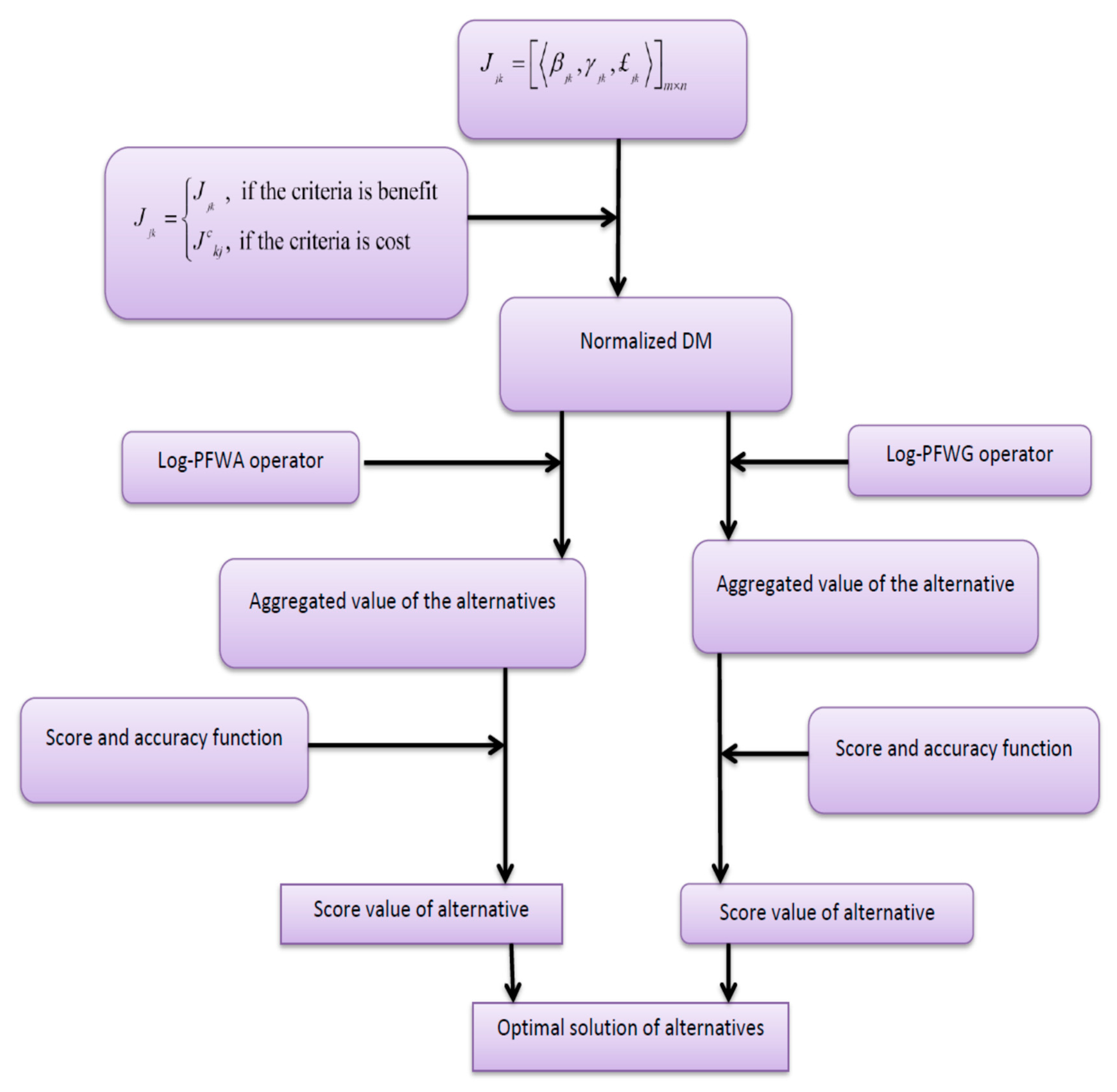
be the decision matrices (DMs), where $\langle {\beta }_{{}_{jk}},{\gamma }_{{}_{jk}},{\pounds }_{{}_{jk}}\rangle$ are the collections of log-PFNs. We also take the weighed vectors of the attribute as $\upsilon ={\left({\upsilon }_1,{\upsilon }_2,\cdots ,{\upsilon }_n\right)}^T$, with ${\upsilon }_{ħ}\in \left[0,1\right],$ and ${\sum }_{ħ=1}^n{\upsilon }_{ħ}=1$. The detail of the propsoed method is given in Figure 1.

We planned the following algorithm to resolve MADM problems with PF information by using the log-PFWA and log-PFWG operators.

Step 1. Normalized the given decision matrices (DMs).

There are two types of criterion one is the benefit criteria and the other one is the cost type criteria. The following equation is used to modify the cost type criteria into benefit criteria. If the given criteria are of the benefit type, then there is no need for normalization:

$$J^c=\langle {\pounds }_{{}_{jk}},{\gamma }_{{}_{jk}},{\beta }_{{}_{jk}}\rangle .$$

Step 2.

In this step, we use the proposed method to aggregate the different preference types of the DMs.

Case 1.The method under the PFN environment is summarized as follows:

$$Log-PFWA\left(J_1,\cdots J_n\right)=\left(1-{\displaystyle \prod _{ħ=1}^n{\left({\log }_{{\tau }_{ħ}}{\beta }_{ħ}\right)}^{{\upsilon }_{ħ}}},{\displaystyle \prod _{ħ=1}^n{\left({\log }_{{\tau }_{ħ}}\left(1-{\gamma }_{ħ}\right)\right)}^{{\upsilon }_{ħ}}},{\displaystyle \prod _{ħ=1}^n{\left({\log }_{{\tau }_{ħ}}\left(1-{\pounds }_{ħ}\right)\right)}^{{\upsilon }_{ħ}}}\right).$$

Case 2.

$$Log-PFWG\left(J_1,\cdots J_n\right)=\left({\displaystyle \prod _{ħ=1}^n{\left(1-{\log }_{{\tau }_{ħ}}{\beta }_{ħ}\right)}^{{\upsilon }_{ħ}}},1-{\displaystyle \prod _{ħ=1}^n{\left(1-{\log }_{{\tau }_{ħ}}\left(1-{\gamma }_{ħ}\right)\right)}^{{\upsilon }_{ħ}}},1-{\displaystyle \prod _{ħ=1}^n{\left(1-{\log }_{{\tau }_{ħ}}\left(1-{\pounds }_{ħ}\right)\right)}^{{\upsilon }_{ħ}}}\right)$$

Case 3.

$$Log-PFOWA\left(J_1,\cdots J_n\right)=\left(\begin{array}{c}1-{\displaystyle \prod _{ħ=1}^n{\left({\log }_{{\tau }_{ħ}}{\beta }_{\wp \left(ħ\right)}\right)}^{{\upsilon }_{ħ}}},{\displaystyle \prod _{ħ=1}^n{\left({\log }_{{\tau }_{ħ}}\left(1-{\gamma }_{\wp \left(ħ\right)}\right)\right)}^{{\upsilon }_{ħ}}},\\ {\displaystyle \prod _{ħ=1}^n{\left({\log }_{{\tau }_{ħ}}\left(1-{\pounds }_{\wp \left(ħ\right)}\right)\right)}^{{\upsilon }_{ħ}}}\end{array}\right)$$

Case 4.

$$Log-PFOWG\left(J_1,\cdots J_n\right)=\left(\begin{array}{c}{\displaystyle \prod _{ħ=1}^n{\left(1-{\log }_{{\tau }_{ħ}}{\beta }_{\wp \left(ħ\right)}\right)}^{{\upsilon }_{ħ}}},1-{\displaystyle \prod _{ħ=1}^n{\left(1-{\log }_{{\tau }_{ħ}}\left(1-{\gamma }_{\wp \left(ħ\right)}\right)\right)}^{{\upsilon }_{ħ}}},\\ 1-{\displaystyle \prod _{ħ=1}^n{\left(1-{\log }_{{\tau }_{ħ}}\left(1-{\pounds }_{\wp \left(ħ\right)}\right)\right)}^{{\upsilon }_{ħ}}}\end{array}\right)$$

Step 3.

In this step, we use Definition 5 to calculate the score and accuracy functions of the decision matrices.

Step 4.

In this step, we rank the alternatives based on score and accuracy functions to choose the best option.

5. Descriptive Example

In this section, the proposed method is applied to a circulation center evaluation problem. Consider a committee of DMs to evaluate and select the most suitable circulation center among four circulation centers: $G_1,G_2,G_3$, and $G_4$. The decision maker evaluates the four circulation center alternatives based on four aspects: cost of transportation $(u_1),$ load of capacity $(u_2),$ satisfying demand with minimum delay $(u_3)$, and security $(u_4)$. We selected the best option according to the suitability ratings of the four alternatives, $G_1,G_2,G_3$ and $G_4$, under four aspects $u_1,u_2,u_3$, and $u_4$ whose weight vector is (0.224, 0.236, 0.304, 0.236), which are assumed by DM. In this example, the DM is designed to be $G={\left(J_{mn}\right)}_{4\times 4}$, as shown in

Table 1. Petroleum circulation center information.

	$u_1$	$u_2$	$u_3$	$u_4$
$G_1$	(0.25, 0.30, 0.40)	(0.27, 0.25, 0.35)	(0.40, 0.20, 0.20)	(0.45, 0.15, 0.10)
$G_2$	(0.17, 0.23, 0.45)	(0.26, 0.32, 0.38)	(0.42, 0.11, 0.10)	(0.35, 0.30, 0.23)
$G_3$	(0.12, 0.15, 0.25)	(0.10, 0.20, 0.45)	(0.55, 0.35, 0.15)	(0.43, 0.30, 0.20)
$G_4$	(0.24, 0.28, 0.37)	(0.25, 0.23, 0.33)	(0.42, 0.11, 0.19)	(0.41, 0.15, 0.09)

.

Step 1. First, we normalized the DM in

Table 2. Normalized petroleum circulation center information.

	$u_1$	$u_2$	$u_3$	$u_4$
$G_1$	(0.40, 0.30, 0.25)	(0.35, 0.25, 0.27)	(0.40, 0.20, 0.20)	(0.45, 0.15, 0.10)
$G_2$	(0.45, 0.23, 0.17)	(0.38, 0.32, 0.26)	(0.42, 0.11, 0.10)	(0.35, 0.30, 0.23)
$G_3$	(0.25, 0.15, 0.12)	(0.45, 0.20, 0.10)	(0.55, 0.35, 0.15)	(0.43, 0.30, 0.20)
$G_4$	(0.37, 0.28, 0.24)	(0.33, 0.23, 0.25)	(0.42, 0.11, 0.19)	(0.41, 0.15, 0.09)

.

Step 2. Operate the aggregation operator to evaluate the DMs of the logarithm picture fuzzy information.

Case 1. Using the Log-PFWA operator, we have

Table 3. Petroleum circulation center information.

$G_1$	(0.6022, 0.1060, 0.0931)
$G_2$	(0.6032, 0.1047, 0.0825)
$G_3$	(0.6361, 0.1231, 0.0650)
$G_4$	(0.5857, 0.0835, 0.0864)

.

Case 2. In this case, we are using the Log-PFWG, we have

Table 4. Petroleum circulation center information.

$G_1$	(0.5990, 0.1111, 0.1013)
$G_2$	(0.5994, 0.1184, 0.0906)
$G_3$	(0.6027, 0.1336, 0.0680)
$G_4$	(0.5822, 0.0915, 0.0942)

.

Case 3. In this case, we use the Log-PFOWA. We have

Table 5. Petroleum circulation center information.

$G_1$	(0.6016, 0.1104, 0.0959)
$G_2$	(0.6005, 0.1146, 0.0892)
$G_3$	(0.6248, 0.1210, 0.0666)
$G_4$	(0.5813, 0.0904, 0.0891)

.

Case 4. In this case, we use the Log-PFOWG. We have

Table 6. Petroleum circulation center information.

$G_1$	(0.5985, 0.1160, 0.1041)
$G_2$	(0.5968, 0.1269, 0.1060)
$G_3$	(0.5929, 0.1309, 0.0699)
$G_4$	(0.5780, 0.0986, 0.0970)

.

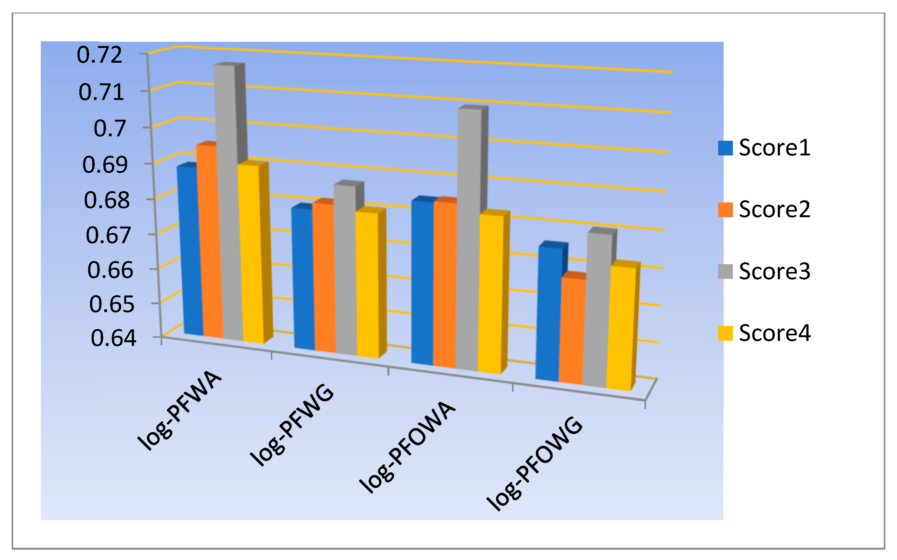
Step 3. In this step, we compute the score values using definition 5, $S(G_m)(m=1,\dots ,4)$ of the Log-PFNs, as shown in

Table 7. Alternative ranking.

	S (${\mathit{G}}_{\mathbf{1}}$)	S (${\mathit{G}}_{\mathbf{2}}$)	S (${\mathit{G}}_{\mathbf{3}}$)	S (${\mathit{G}}_{\mathbf{4}}$)	Ranking
Log-PFWA	0.6886	0.6950	0.7172	0.6905	$G_3>G_2>G_4>G_1$
Log-PFWG	0.6798	0.6817	0.6872	0.6804	$G_3>G_2>G_4>G_1$
Log-PFOWA	0.6847	0.6850	0.7097	0.6827	$G_3>G_2>G_1>G_4$
Log-PFOWG	0.6757	0.6682	0.6805	0.6725	$G_3>G_1>G_4>G_2$

.

Step 4. Thus, the best petroleum circulation center is $G_3$.

The comparison of the alternative based on score values is shown in Figure 2.

5.1. Comparison Analysis with the Existing Methods

This section provides our comparison analysis of the existing aggregation operators and our novel logarithmic aggregation operators. The existing aggregation operators were proposed by Ashraf et al. [23] in 2018 to handle picture fuzzy quantities. Ashraf introduced the picture fuzzy aggregation operators, such as picture fuzzy geometric, order geometric, and hybrid geometric aggregation operators. We provide novel aggregation operators including logarithmic picture averaging and geometric aggregation operators, such as logarithmic picture fuzzy average, ordered average, geometric, and ordered geometric aggregation operators. The logarithmic aggregation operators proposed in this paper are more general, more accurate, and more flexible.

To evaluate air quality, we take the descriptive example proposed by Ashraf et al. [23]. Three stations are used to evaluate the air quality, denoted as ($O_1$, $O_2$, $O_3$). Decision maker weights are ${(0.314,0.355,0.331)}^T$. We have three criteria’s $C_1,C_2 and C_3$. The collected information from these three stations, which is given in the

Table 8. Air quality data from station O₁.

	$C_1$	$C_2$	$C_3$
$G_1$	($0.265,0.150,0.385$)	($0.330,0.190,0.280$)	($0.245,0.175,0.380$)
$G_2$	($0.345,0.145,0.310$)	($0.430,0.190,0.180$)	($0.245,0.275,0.310$)
$G_3$	($\langle 0.365,0.150,0.335$)	($0.480,0.310,0.105$)	($0.340,0.310,0.190$)
$G_4$	($0.430,0.210,0.170$)	($0.460,0.145,0.165$)	($0.310,0.430,0.070$)

,

Table 9. Air quality data from station O₂.

	$C_1$	$C_2$	$C_3$
$G_1$	($0.125,0.470,0.200$)	($0.220,0.400,0.160$)	($0.345,0.410,0.125$)
$G_2$	($0.355,0.335,0.120$)	($0.300,0.170,0.330$)	($0.205,0.430,0.105$)
$G_3$	($0.315,0.380,0.100$)	($0.340,0.265,0.195$)	($0.280,0.520,0.190$)
$G_4$	($0.365,0.375,0.135$)	($0.355,0.220,0.305$)	($0.325,0.405,0.090$)

and

Table 10. Air quality data from station O₃.

	$C_1$	$C_2$	$C_3$
$G_1$	($0.260,0.075,0.395$)	($0.220,0.414,0.160$)	($0.255,0.370,0.275$)
$G_2$	($0.270,0.160,0.360$)	($0.320,0.015,0.465$)	($0.135,0.575,0.090$)
$G_3$	($0.245,0.365,0.290$)	($0.250,0.570,0.110$)	($0.175,0.330,0.165$)
$G_4$	($0.390,0.340,0.160$)	($0.305,0.435,0.120$)	($0.465,0.425,0.076$)

.

Step 2.

In this step, we use the proposed $Log-PFWA$ aggregation operator to evaluate the collective picture fuzzy matrix, which is in shown in

Table 11. Collective picture fuzzy information.

	$C_1$	$C_2$	$C_3$
$G_1$	($0.3205,0.0897,0.1619$)	($0.4037,0.1705,0.0923$)	($0.4519,0.1597,0.1157$)
$G_2$	($0.5097,0.0990,0.1173$)	($0.5407,0.0366,0.1617$)	($0.2836,0.2354,0.0667$)
$G_3$	($0.4869,0.1454,0.1034$)	($0.5489,0.1979,0.0621$)	($0.4176,0.2105,0.0869$)
$G_4$	($0.5652,0.1577,0.0724$)	($0.5700,0.1229,0.0896$)	($0.5645,0.2361,0.0355$)

and

Table 12. (a) Ordered collective picture fuzzy information. (b) Aggregated information.

(a)
	$C_1$	$C_2$	$C_3$
$G_1$	($0.4519,0.1597,0.1157$)	($0.4037,0.1705,0.0923$)	($0.3205,0.0897,0.1619$)
$G_2$	($0.5407,0.0366,0.1617$)	($0.5097,0.0990,0.1173$)	($0.2836,0.2354,0.0667$)
$G_3$	($0.5489,0.1979,0.0621$)	($0.4869,0.1454,0.1034$)	($0.4176,0.2105,0.0869$)
$G_4$	($0.5700,0.1229,0.0896$)	($0.5652,0.1577,0.0724$)	($0.5645,0.2361,0.0355$)
(b)
G1	(0.5927, 0.0632, 0.0553)
G2	(0.6501, 0.0448, 0.0496)
G3	(0.6853, 0.0868, 0.0377)
G4	(0.7531, 0.0795, 0.0274)

.

Next, we operate the $Log-PFOWA$ aggregation operator, to rank the alternatives.

Step 3. In this step, we compute the score values using definition 5. $S(G_m)(m=1,\dots ,4)$ of the Log-PFNs is as shown in

Table 13. $\mathrm{Evaluation} \mathrm{results} \mathrm{of} \mathrm{each} \mathrm{air} \mathrm{station}$.

	$Log-PFOWA$
$\mathrm{Score}$	$sco(G_4)=0.828>sco(G_3)=0.779>sco(G_2)=0.770>sco(G_1)=0.7197$
$\mathrm{Ranking}$	$G_4>G_3>G_2>G_1$

.

Step 4. Thus, the best evaluation result for this case is $G_4$.

We compared the existing method [23] and our novel logarithmic aggregation operators. From the analysis, we found our proposed aggregation operator (log-PFOWA) and the existing method aggregation operator [23] provide the same result, as shown in

Table 14. Comparison analysis with the existing method [23].

Method	Ranking Order
Ashraf [23],	$G_4>G_3>G_2>G_1$
Log-PFOWA (introduced method)	$G_4>G_3>G_2>G_1$

.

Table 14 shows that our proposed method logarithmic picture fuzzy aggregation operator provides new method to find the best alternative in this decision-making problem.

6. Conclusions

In this paper, we outlined the logarithmic operational laws of PFNs, which are a useful supplement to the existing picture fuzzy aggregation techniques. Based on the logarithmic operational laws, we constructed a series of aggregation operators of PFNs, i.e., Log-PFWA, Log-PFWG, Log-PFOWA, and Log-PFOWG. Several characteristics required of these logarithmic aggregation operators were comprehensively explored. To demonstrate the efficiency and consistency of the proposed picture fuzzy logarithmic aggregation operators, we developed an algorithm to address MADM problems for tacking the uncertainty in the form of picture fuzzy information. A descriptive example using a circulation center evaluation problem was provided to validate and demonstrate the applicability of our proposed technique. Consequently, we also demonstrated the superiority and the validity of the proposed aggregation operators using some of the existing tools. Hence, the analysis showed that our proposed aggregation operator is more reliable and accurate than the existing method. Thus, our proposed method logarithmic aggregation operator provides new method to find the best alternative in the MADM decision-making problem.

In future work, we will discuss the generalized form of these operators for the logarithmic operational law of PFSs and define the hybrid averaging and hybrid geometric operators.

References

1. Attanassov, K. Intuitionistic fuzzy sets. Fuzzy Sets Syst. 1986, 20, 87–96. [Google Scholar] [CrossRef]
2. Zadeh, L.A. Fuzzy sets. Inf. Control 1965, 8, 338–353. [Google Scholar] [CrossRef] [Green Version]
3. Xu, Z.; Chen, J.; Wu, J. Clustering algorithm for intuitionistic fuzzy sets. Inf. Sci. 2008, 178, 3775–3790. [Google Scholar] [CrossRef]
4. Hong, D.H.; Choi, C.H. Multi criteria fuzzy decision-making problems based on vague set theory. Fuzzy Sets Syst. 2000, 114, 103–113. [Google Scholar] [CrossRef]
5. De, S.K.; Biswas, R.; Roy, A.R. An application of intuitionistic fuzzy sets in medical diagnosis. Fuzzy Sets Syst. 2001, 117, 209–213. [Google Scholar] [CrossRef]
6. Khatibi, V.; Montazer, G.A. Intuitionistic fuzzy set vs. fuzzy set application in medical pattern recognition. Artif. Intell. Med. 2009, 47, 43–52. [Google Scholar] [CrossRef]
7. Chen, S.M.; Chang, C.H. Fuzzy multi attribute decision making based on transformation techniques of intuitionistic fuzzy values and intuitionistic fuzzy geometric averaging operators. Inf. Sci. 2016, 352, 133–149. [Google Scholar] [CrossRef]
8. Garg, H. Some robust improved geometric aggregation operators under interval-valued intuitionistic fuzzy environment for multi-criteria decision-making process. J. Ind. Manag. Optim. 2018, 14, 283–308. [Google Scholar] [CrossRef] [Green Version]
9. Huang, J.Y. Intuitionistic fuzzy Hamacher aggregation operators and their application to multiple attribute decision making. J. Intell. Fuzzy Syst. 2014, 27, 505–513. [Google Scholar]
10. Chen, S.M.; Cheng, S.H.; Tsai, W.H. Multiple attribute group decision making based on interval-valued intuitionistic fuzzy aggregation operators and transformation techniques of interval valued intuitionistic fuzzy values. Inf. Sci. 2016, 368, 418–442. [Google Scholar] [CrossRef]
11. Wang, W.; Liu, X. The multi-attribute decision making method based on interval-valued intuitionistic fuzzy Einstein hybrid weighted geometric operator. Comput. Math. Appl. 2013, 66, 1845–1856. [Google Scholar] [CrossRef]
12. Yager, R. Pythagorean fuzzy subsets. In Proceedings of the Joint IFSA World Congress and NAFIPS Annual Meeting, Edmonton, AB, Canada, 24–28 June 2013; pp. 57–61. [Google Scholar]
13. Yager, R. Pythagorean membership grades in multi attribute decision making. IEEE Trans. Fuzzy Syst. 2014, 22, 958–965. [Google Scholar] [CrossRef]
14. Khan, A.A.; Ashraf, S.; Abdullah, S.; Qiyas, M.; Luo, J.; Khan, S.U. Pythagorean Fuzzy Dombi Aggregation Operators and Their Application in Decision Support System. Symmetry 2019, 11, 383. [Google Scholar] [CrossRef]
15. Zhang, X. A novel approach based on similarity measure for Pythagorean fuzzy multiple attribute group decision making. Int. J. Intell. Syst. 2016, 31, 593–611. [Google Scholar] [CrossRef]
16. Cuong, B.C.; Kreinovich, V. December. Picture Fuzzy Sets-a new concept for computational intelligence problems. In Proceedings of the 2013 Third World Congress on Information and Communication Technologies (WICT 2013), Hanoi, Vietnam, 15–18 December 2013; IEEE, 2015; pp. 1–6. [Google Scholar]
17. Phong, P.H.; Hieu, D.T.; Ngan, R.T.; Them, P.T. Some compositions of picture fuzzy relations. In Proceedings of the 7th National Conference on Fundamental and Applied Information Technology Research, Thai Nguyen, Vietnam, 19 June 2014; pp. 19–20. [Google Scholar]
18. Singh, P. Correlation coefficients for picture fuzzy sets. J. Intell. Fuzzy Syst. 2015, 28, 591–604. [Google Scholar]
19. Cuong, B.C.; Van Hai, P. Some fuzzy logic operators for picture fuzzy sets. In Proceedings of the 2015 Seventh International Conference on Knowledge and Systems Engineering, Ho Chi Minh City, Vietnam, 8–10 October 2015; pp. 132–137. [Google Scholar]
20. Thong, P.H. A new approach to multi-variable fuzzy forecasting using picture fuzzy clustering and picture fuzzy rule interpolation method. In Knowledge and Systems Engineering; Springer: Cham, Switzerland, 2015; pp. 679–690. [Google Scholar]
21. Son, L.H. Generalized picture distance measure and applications to picture fuzzy clustering. Appl. Soft Comput. 2016, 46, 284–295. [Google Scholar] [CrossRef]
22. Wei, G. Picture fuzzy cross-entropy for multiple attribute decision making problems. J. Bus. Econ. Manag. 2016, 17, 491–502. [Google Scholar] [CrossRef]
23. Ashraf, S.; Mahmood, T.; Abdullah, S.; Khan, Q. Different approaches to multi-criteria group decision making problems for picture fuzzy environment. Bull. Braz. Math. Soc. New Ser. 2019, 50, 373–397. [Google Scholar] [CrossRef]
24. Garg, H. Some picture fuzzy aggregation operators and their applications to multi criteria decision-making. Arab. J. Sci. Eng. 2017, 42, 5275–5290. [Google Scholar] [CrossRef]
25. Wei, G. Picture fuzzy aggregation operators and their application to multiple attribute decision making. J. Intell. Fuzzy Syst. 2017, 33, 713–724. [Google Scholar] [CrossRef]
26. Zeng, S.; Ashraf, S.; Arif, M.; Abdullah, S. Application of Exponential Jensen Picture Fuzzy Divergence Measure in Multi-Criteria Group Decision Making. Mathematics 2019, 7, 191. [Google Scholar] [CrossRef]
Figure 1. Graphically presentation of the proposed method.
Mathematics 07 00608 g001
Figure 2. Score comparison of alternatives.
Mathematics 07 00608 g002