Long-Time Asymptotics of a Three-Component Coupled mKdV System


1
Department of Mathematics, Zhejiang Normal University, Jinhua 321004, China
2
Department of Mathematics, King Abdulaziz University, Jeddah 21589, Saudi Arabia
3
Department of Mathematics and Statistics, University of South Florida, Tampa, FL 33620, USA
4
College of Mathematics and Physics, Shanghai University of Electric Power, Shanghai 200090, China
5
College of Mathematics and Systems Science, Shandong University of Science and Technology, Qingdao 266590, China
6
International Institute for Symmetry Analysis and Mathematical Modelling, Department of Mathematical Sciences, North-West University, Mafikeng Campus, Private Bag X2046, Mmabatho 2735, South Africa
Mathematics 2019, 7(7), 573; https://doi.org/10.3390/math7070573
Submission received: 2 June 2019
/
Revised: 10 June 2019
/
Accepted: 20 June 2019
/
Published: 27 June 2019
Abstract
:We present an application of the nonlinear steepest descent method to a three-component coupled mKdV system associated with a matrix spectral problem. An integrable coupled mKdV hierarchy with three potentials is first generated. Based on the corresponding oscillatory Riemann-Hilbert problem, the leading asympototics of the three-component mKdV system is then evaluated by using the nonlinear steepest descent method.
MSC:
35Q53; 37K10; 37K201. Introduction
Asymptotic analysis has become an important area in soliton theory and its basic approaches are used to determine limiting behaviors of Cauchy problems of integrable systems. Significant work on long-time asympototics of integrable systems was carried out by Manakov [1] and Ablowitz and Newell [2]. Zakharov and Manakov [3] wrote down precise expressions, depending explicitly on initial data, for the leading asymptotics for the nonlinear Schrödinger equation in the physically interesting region . A complete description was presented for the leading asymptotics of the Cauchy problem of the Korteweg-de Vries (KdV) equation by Ablowitz and Segur [4]. The method of Zakharov and Manakov starts an ansatz for the asymptotic form of the solution and utilizes some techniques which are removed from the classical framework of Riemann-Hilbert (RH) problems. Segur and Ablowitz [5] began with the similarity solution form to derive the leading two terms in each of the asymptotic expansions for the amplitude and phase for the nonlinear Schrödinger equation, based on conservation laws. However, all those results were presented, without applying the method of stationary phase.
Its [6] used the stationary phase idea to conjugate the RH problem associated with the nonlinear Schrödinger equation, up to small errors which decay as , by an appropriate parametrix to a model RH problem solvable by the technique from the theory of isomonodromic deformations. Deift and Zhou [7] determined the long-time asymptotics of the mKdV equation, by manipulating an associated oscillatory RH problem systematically and rigorously, in the spirit of the stationary phase method. Their technique, further developed in [8,9] and also in [10], opens a nonlinear steepest descent method to explore asymptotics of integrable systems through analyzing oscillatory RH problems associated with matrix spectral problems. A crucial ingredient of the Deift-Zhou approach is the asymptotic analysis of singular integrals on contours by deformations. Applications have been made for a few of integrable equations, including the KdV equation, the nonlinear Schrödinger equation, the sine-Gordon equation, the derivative nonlinear Schrödinger equation, the Camassa-Holm equation and the Kundu-Eckhaus equation (see, e.g., [11,12,13,14,15,16,17,18]). McLaughlin and Miller [19] generalized the steepest descent method to the case when the jump matrix fails to be analytic and their method is now called a nonlinear steepest descent method. One important factor in the nonlinear steepest descent method is the order of involved spectral matrices in RH problems or equivalently the inverse scattering theory. However, only spectral matrices and their RH problems have been systematically considered (see, e.g., [20]), which lead to algebro-geometric solutions to integrable systems expressed by hyperelliptic functions [21]. There are very few spectral matrices, whose long-time asymptotics or RH problems are considered (see, e.g., [22,23]) and whose associated inverse scattering transforms are solved (see, e.g., [24,25]). Associated trigonal curves exhibit much more diverse asymptotic behaviors and algebro-geometric solutions than hyperelliptic curves [26,27]. There has been no application of the nonlinear steepest descent method to the 4th-order or higher-order matrix spectral problems so far.
In this paper, we would like to present an application to a matrix spectral problem
where i denotes the unit imaginary number, k is the spectral parameter and the superscript ∗ denotes the complex conjugate. This spectral problem generates a three-component coupled mKdV system
where
We will compute the leading asymptotics of this mKdV system by analyzing an associated oscillatory RH problem. Symmetry constraints and RH problems have been made for an unreduced combined mKdV system in [28,29]. It is worth noting that this mKdV system (2) has a slightly different matrix spectral problem from the one for the multiple wave interaction equations [30].
Let denote an equivalent matrix norm for a matrix M (may not be square):
where stands for the Hermitian transpose of M, and
where denotes the Schwartz space. The primary result of the paper can be stated as follows.
Theorem 1.
Let solves the Cauchy problem of the three-component coupled mKdV system (2) with initial data in . Suppose that is the reflection coefficient vector in associated with the initial data and it satisfies
Then, in the physically interesting region , the leading asymptotics of the solution for is given by
where
being the Gamma function.
The rest of the paper is organized as follows. In Section 2, within the zero-curvature formulation, we derive an integrable coupled hierarchy with three potentials and furnish its bi-Hamiltonian structure, based on the matrix spectral problem (1) suited for the RH theory. In Section 3, taking the three-component coupled mKdV system (2) as an example, we present an associated oscillatory RH problem. In Section 4, we explore long-time asymptotics for the three-component coupled mKdV system through manipulating the oscillatory RH problem by the nonlinear steepest descent method. In the last section, we give a summary of our conclusions, together with some discussions.
2. An Integrable Three-Component Coupled mKdV Hierarchy
2.1. Zero Curvature Formulation
Let us first recall the zero curvature formulation to construct integrable hierarchies [31]. Let u be a vector potential, k be a spectral parameter, and stand for the n-th order identity matrix. Choose a square spectral matrix from a given matrix loop algebra. Suppose that
presents a solution to the corresponding stationary zero curvature equation
By using the solution W, we define an infinite sequence of Lax matrices
where the subscript + denotes the operation of taking a polynomial part in k, and , , are appropriate modification terms, and then construct an integrable hierarchy
from an infinite sequence of zero curvature equations
The two matrices U and here are called a Lax pair [32] of the r-th integrable system in the soliton hierarchy (9). The zero curvature equations in (10) present the compatibility requirements of the spatial and temporal matrix spectral problems
with being the matrix eigenfunction.
To show the Liouville integrability of the soliton hierarchy (9), we usually furnish a bi-Hamiltonian structure [33]:
where and constitute a Hamiltonian pair and is the variational derivative. The Hamiltonian structures are normally achieved through the trace identity [31]:
or more generally, the variational identity [34]:
with being a symmetric and ad-invariant non-degenerate bilinear form on the underlying matrix loop algebra [35]. The bi-Hamiltonian structure often guarantees the existence of infinitely many commuting Lie symmetries and conserved quantities :
and
where , or , and denotes the Gateaux derivative of K with respect to the potential u:
Such Abelian algebras of symmetries and conserved quantities can be generated directly from Lax pairs (see, e.g., [36,37]). We also know that for a system of evolution equations,
is a conserved functional if and only if is an adjoint symmetry [38], and thus, Hamiltonian structures connect conserved functionals with adjoint symmetries and further symmetries. Pairs of adjoint symmetries and symmetries actually correspond to conservation laws [39].
When the underlying matrix loop algebra in the zero curvature formulation is simple, semisimple and non-semisimple, the associated zero curvature equations generate classical integrable hierarchies [40,41], a collection of different integrable hierarchies, and hierarchies of integrable couplings [42], respectively. Integrable couplings require extra care in presenting lumps and solitons.
2.2. Three-Component mKdV Hierarchy
Let us consider a matrix spectral problem
where k is a spectral parameter and is a three-component potential. A special case of transforms (17) into the Manakov type spectral problem [43]. Since the leading matrix has a multiple eigenvalue, the spectral problem (17) is degenerate, which is different from the case of multiple wave interaction equations [30].
To derive an associated integrable coupled mKdV hierarchy, we first solve the stationary zero curvature Equation (7) corresponding to (17). We assume that a solution W is determined by
where a is a real scalar, b is a three-dimensional row, and d is a Hermitian matrix. It is direct to observe that the stationary zero curvature Equation (7) becomes
We search for a formal series solution as follows:
with and being assumed to be
Obviously, the system (19) is equivalent to the following recursion relations:
The three-component mKdV system (2) can correspond to the specific initial values:
Besides those initial values, we set all constants of integration in (22c) to be zero, that is, demand
This way, with and given by (23), all matrices , will be uniquely determined. For instance, by a direct computation, (22) generates
where . Based on (22b) and (22c), we can obtain a recursion relation for and :
where is a matrix operator
with . Obviously, this tells
To generate an integrable coupled mKdV hierarchy with three components, we introduce, for all integers , the following Lax matrices
where the modification terms are chosen as zero. The compatibility requirements of (11), i.e., the zero curvature equations (10), lead to the integrable coupled mKdV hierarchy with three components:
The first two nonlinear systems in the above integrable coupled mKdV hierarchy (30) are the three-component coupled nonlinear Schrödinger system
and the three-component coupled mKdV system (2). Under a reduction , the three-component coupled system (31) is reduced to the Manakov system [43], for which a decomposition into finite-dimensional integrable Hamiltonian systems was made in [44], whileas the three-component coupled system (2) contains various examples of mKdV equations, for which there are diverse kinds of integrable decompositions through symmetry constraints (see, e.g., [45,46]).
The three-component coupled mKdV hierarchy (30) with an extended six-component potential possesses a Hamiltonian structure [29,38], which can be computed through applying the trace identity [31], or more generally, the variational identity [34]. A direct computation tells
and
where and . Plugging these into the corresponding trace identity and considering the case of tell , and thus
where . A bi-Hamiltonian structure for the extended six-component coupled mKdV systems, consisting of (30) and its conjugate compartment, then follows:
where the Hamiltonian pair is defined by
where again. Adjoint symmetry constraints (or equivalently symmetry constraints) decompose a four-component nonlinear Schrödinger system with into two commuting finite-dimensional Liouville integrable Hamiltonian systems in [38]. In the next section, we will concentrate on the three-component coupled mKdV system (2).
3. An Associated Oscillatory Riemann-Hilbert Problem
For a matrix , we define
where is the matrix norm of M given by (3) and is the -norm of a function f of k. We assume that as ,
If the constant C depends on a few parameters , then we write , but on some situations where the dependence of C on some parameters is not important, we will often suppress those parameters for brevity.
For an oriented contour, we denote the left-hand side by + and the right-hand side by −, as one travels on the contour in the direction of the arrow. A Riemann-Hilbert (RH) problem on an oriented contour (open or closed) with a jump matrix J defined on reads
where is a given matrix determining a boundary condition at infinity, and are analytic in the ± side regions and continuous to from the ± sides, and in the ± side regions, respectively.
3.1. An Equivalent Matrix Spectral Problem
In the previous section, we have seen that the spectral problems of the three-component coupled mKdV system (2) read
with the Lax pair being of the form
where and
The other two matrices P and Q are given by
where , , are defined in (25), and thus
As normal, for the spectral problems in (38), upon making the variable transformation
we can impose the canonical normalization condition:
The equivalent pair of matrix spectral problems reads
where and . Noting , we have
by a generalized Liouville’s formula [47].
Applying the method of variation in parameters, and using the canonical normalization condition (44), we can transform the x-part of (38) into the following Volterra integral equations for [48]:
Similarly, we can turn the t-part of (38) into the following Volterra integral equations:
Observing the structures of and , we can know that the first column of and the last three columns of consist of analytical functions in the upper half plane , and the first column of and the last three columns of consist of analytical functions in the lower half plane (also see [29,49]). All this will help us formulate an associated RH problem for the three-component coupled mKdV system (2).
3.2. An Oscillatory Riemann-Hilbert Problem
The scattering matrix S is determined by
where for a scalar and two same order square matrices M and X. We also adopt the simple expressions
for a matrix M depending on . Because
we have
and
Notice that due to . It then follows from and (55) that
where is the adjoint matrix of M, and S is the block matrix
with being a matrix. Thus, the scattering matrix S can be written as
where is a matrix.
Introduce
where and denote the first column and the rest columns of . This matrix M solves an associated oscillatory RH problem
where and
with
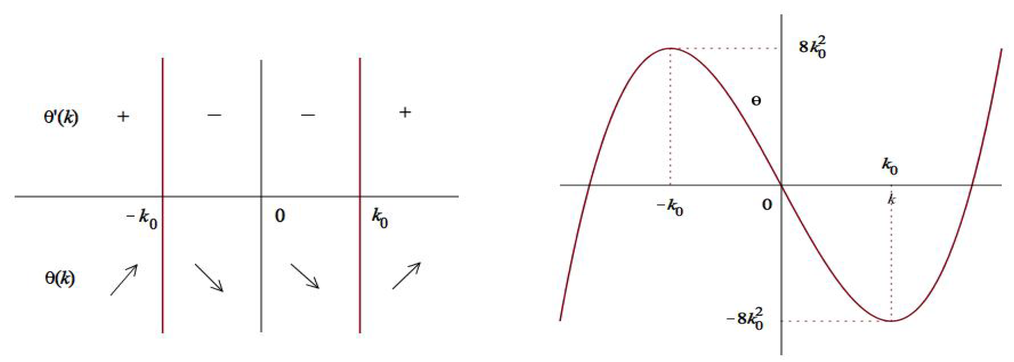
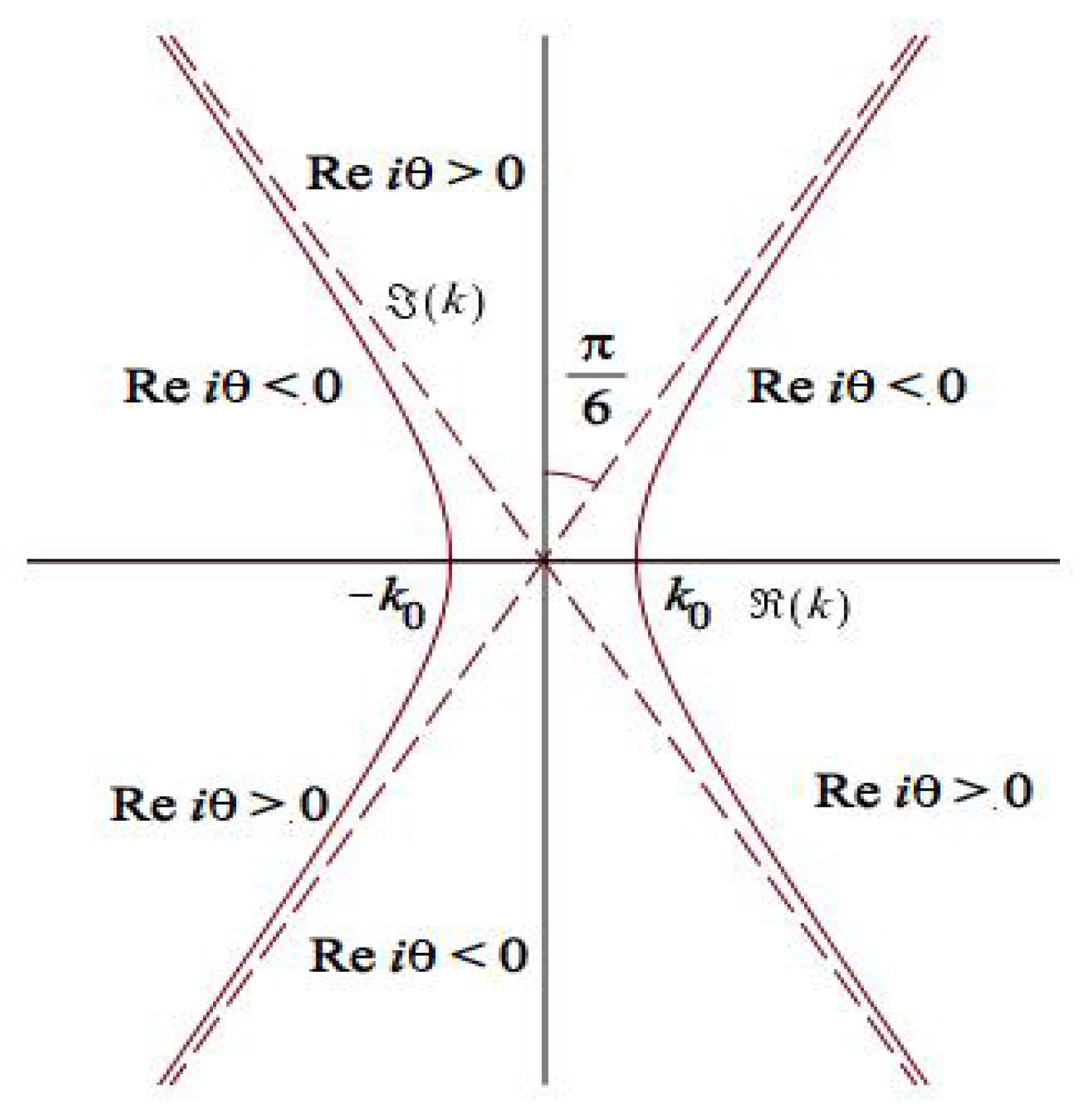
In the above RH problem, we assume that the matrix is invertible, and so we will only analyze the solitonless case. The behavior of the oscillatory factor
depends on the increasing and decreasing of and the signature of (see Figure 1 and Figure 2).
In what follows, we assume that lies in and satisfies
The analysis on RH problems in [50] shows that the above RH problem (58) is equivalent to a Fredholm integral equation of the second kind. For such Fredholm equations, the existences and uniqueness of solutions can be guaranteed by the vanishing lemma [51]. A direct computation also shows [29] that one can compute the potential through the solution to the RH problem (58) as follows.
4. Long-Time Asymptotic Behavior
We will first deal with the Riemann-Hilbert (RH) problem (58) and then compute the long-time aymptotics of the three-component coupled mKdV system (2) with the leading term, by using the nonlinear steepest descent method [7]. We will be concentrated on the physically interesting region , where C is a positive constant.
4.1. Transformation of the RH Problem
Obviously, the jump matrix J has the following upper-lower and lower-upper factorizations:
and
We would like to introduce another RH problem to replace the upper-lower factorization with the lower-upper factorization to make the analytic and decay properties of the two factorizations consistent.
We easily see that the stationary points of are where , by computing . Let solve the RH problem
which implies a scalar RH problem
noting that
Due to (61), the jump matrix is positive definite. Thus, it follows from the vanishing lemma (see, e.g., [51]) that the RH problem (65) has a unique solution . In addition, the Plemelj formula [51] gives the unique solution of the above scalar RH problem (66):
where
By the uniqueness, we obtain
It then follows that
and
Therefore, by the maximum principle for analytic functions, we can have
from the canonical normalization condition of the above two RH problems.
Let us now introduce
and a vector-valued spectral induced function
Denote by
and reverse the orientation for as shown in Figure 3.
4.2. Decomposition of the Spectral Induced Function
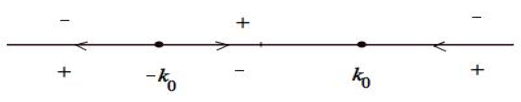
To determine the required deformation, we first make a decomposition of the spectral induced function . By L, we denote the contour
and by , denote the contour
with the orientation in Figure 4.
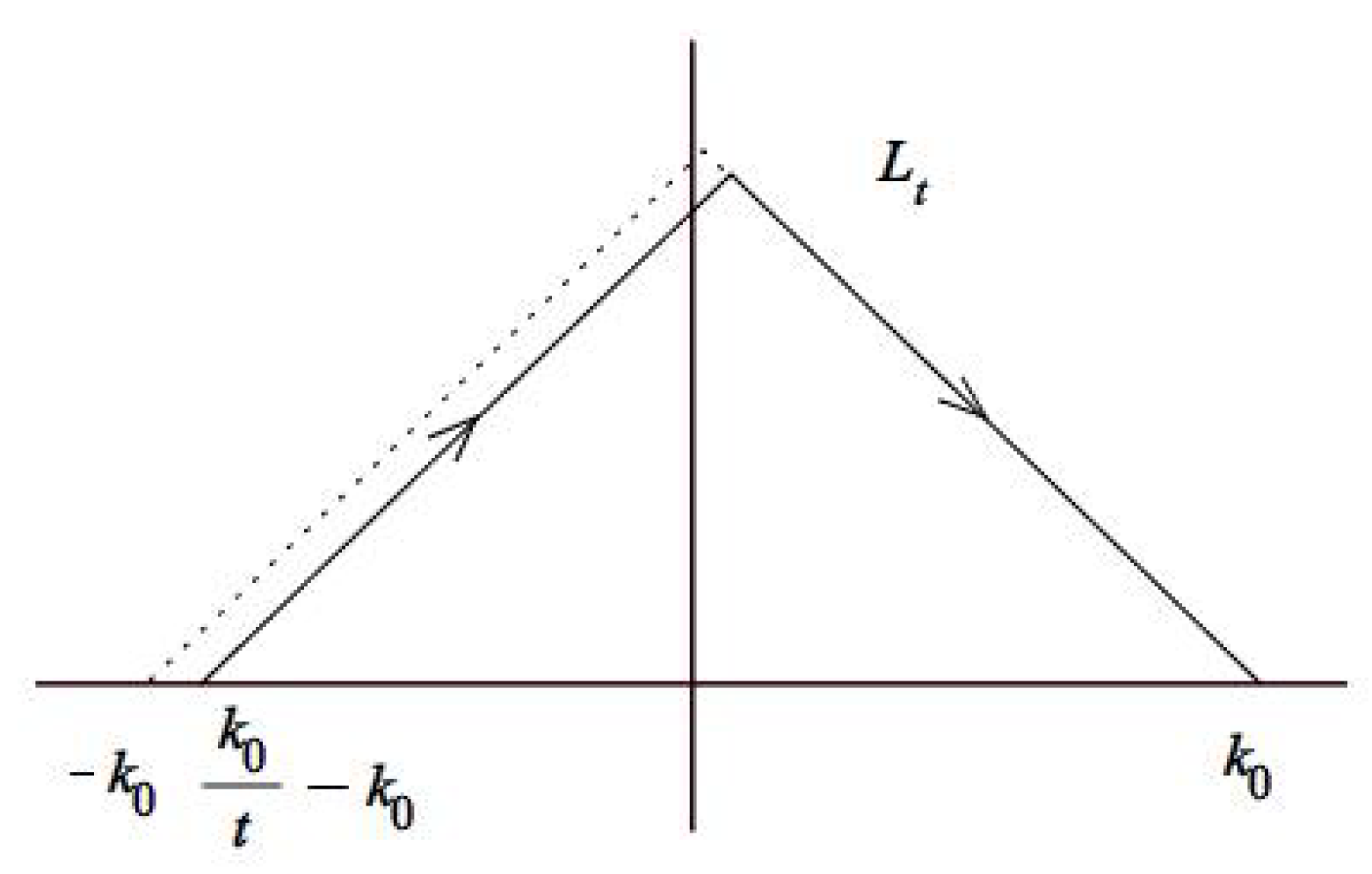
Further let denote the following part of the contour L:
where . We will focus on the contour , though any other contour of the same shape as , which locates in the the region where is positive, will work.
Proposition 1.
The vector-valued spectral induced function has the following decomposition on the real axis:
where is a polynomial on and a rational function on , has an analytic continuation from to L in the region where , and and R have the estimates as :
where l is an arbitrary positive integer. Taking the Hermitian conjugate
yields the same estimates for and on and , respectively.
Proof.
Throughout the proof, we use the differential notation for brevity, while dealing with the Fourier transform. We only consider the physically interesting region and so is bounded. Let r be a fixed positive integer.
(a) First, we consider the case of . In this case, we have . Splitting it into even and odd parts leads to
where and are two vector functions in . By Taylor’s theorem with the integral form of the remainder, we have
and
Set
Then, we have
and the coefficients
decay rapidly as .
We assume that r is of form
with an even number q. Express
By the characteristic of R in (89), we have
Based on this property, we will try to split h into two parts
where is small and has an analytic continuation from to L in the region where . This way, we obtain the required splitting of .
Let us introduce
We consider the Fourier transform with respect to . Because is one-to-one in (see Figure 1), we define
Based on (94), we have
and as , we see that
where the s are Hilbert spaces. It follows from the Fourier inversion theorem that
where is the Fourier transform
By the formulae (86), (87), (88) and (93) we have
Then, it follows that
from which, by the Plancherel theorem, we know
Now make a splitting for h as follows:
On one hand, based on (104) and noting , we have
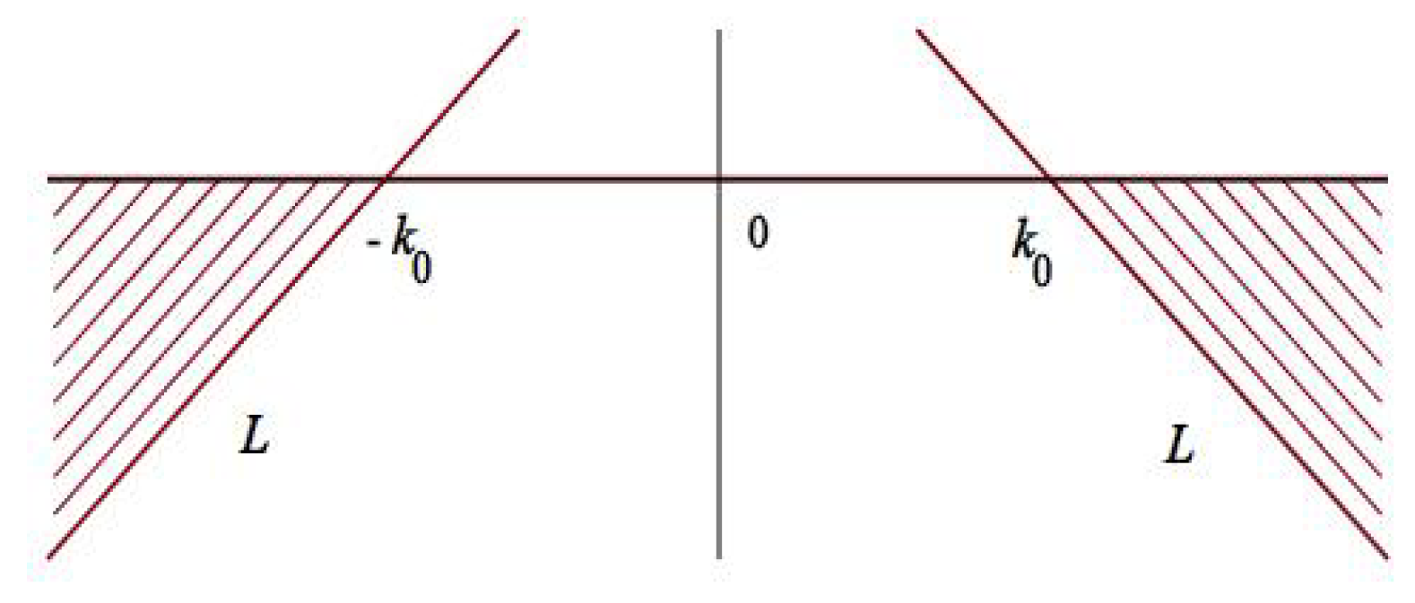
On the other hand, we know that is positive in the hatched region in Figure 5, and thus that has an analytic continuation from to the line segments in the upper half k-plane:
Let k be on the line segment (107). Then, we can have that
again based on (104). But
Therefore, we have
Similarly, we can show that the same estimate holds on the line segment (108).
Finally fix . Then on the parts of the line segments (107) and (108) with away from , we have
(by, e.g., (110) on the line segment (107) and is a polynomial), where .
(b) Second, we consider the case of . We only consider the sub-case , since the other sub-case is completely similar. In this case, we have
Once more, we use Taylor’s theorem to obtain
Define
and set
As before, we know that
and
decay rapidly as .
Similarly, introduce
Following the Fourier inversion theorem, we have
where is the Fourier transform
Based on the formulae (114), (116) and (119), we see that
where
from which it follows that
Noting that
we have
By the Plancherel theorem,
Again, we split
On the other hand, has an analytic continuation from to the ray
in two parts of the lower half k-plane, where , as shown in Figure 6.
Let k be on the ray (130). Similarly as in the previous case , we can show that
However, we have
and thus, we have
since is bounded. This completes the proof of Proposition 1. □
We are now ready to make a deformation of the RH problem (76).
4.3. Deformation of the RH Problem
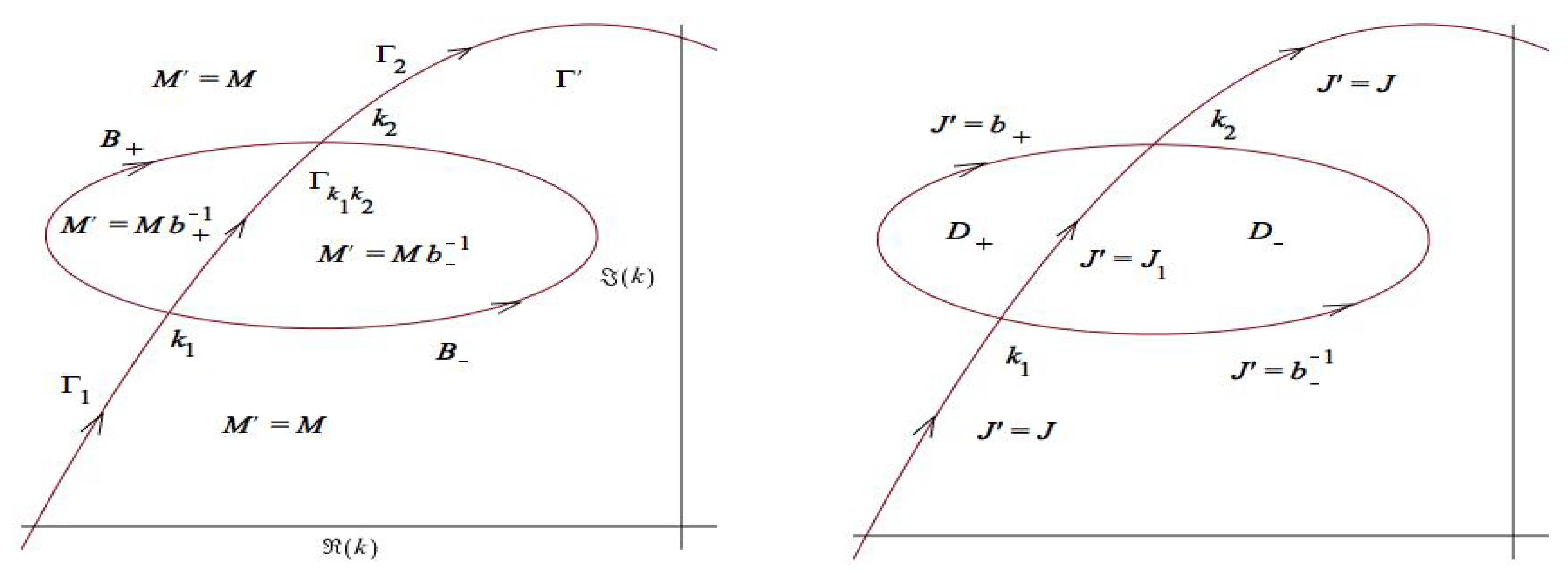
Let us first explain what a deformation of a RH problem is. Suppose that we have a RH problem on an oriented contour (see Figure 7):
and that on a part (which could be the whole contour ) of from to in the direction of , denoted by , we have
where have invertible and analytic continuations to the ± sides of a region D (see Figure 7) supported by and , respectively. Define an extended oriented contour (see Figure 7):
and an extended jump matrix :
Then the RH problem (133) on is equivalent to the following RH problem on :
and the relation between the two solutions reads
It is clear that one RH problem is solvable if and only if the other RH problem is solvable, and the solution to the one problem gives the solution to the other problem automatically by (138). We call a deformation of the original RH problem . If D is not bounded, then we need to require that and tend to the identity matrix as , in order to keep the same normalization condition.
We now deform the RH problem (76) from to the augmented contour . The first important step is to observe that the jump matrix can be rewritten as
where
Moreover, noting the decomposition (81), we have
and thus, the decompositions for :
We can also state that
It finally follows that the jump matrix has the following factorization:
It is now standard to introduce
and then the RH problem (76) on becomes the following new RH problem on :
where
The canonical normalization condition in (148) can be verified, indeed. For example, converges to as in , because we observe that for fixed , by the definition of in (128) and the boundedness of and in (72), we have
and by the definition of R in (115) and the boundedness of and in (72), we have
both of which converge to 0 as in .
The above RH problem (148) can be solved by using the Cauchy operators as follows (see [52,53]). Let us denote by the two Cauchy operators
on . As is well known, these two operators are bounded from to , and satisfy . Define
for a matrix-valued function f, where
Assume that solves the fundamental inverse equation
Then, we can see that
presents the unique solution of the RH problem (148).
Theorem 3.
The solution of the three-component coupled mKdV system (2) is expressed by
4.4. Contour Truncation
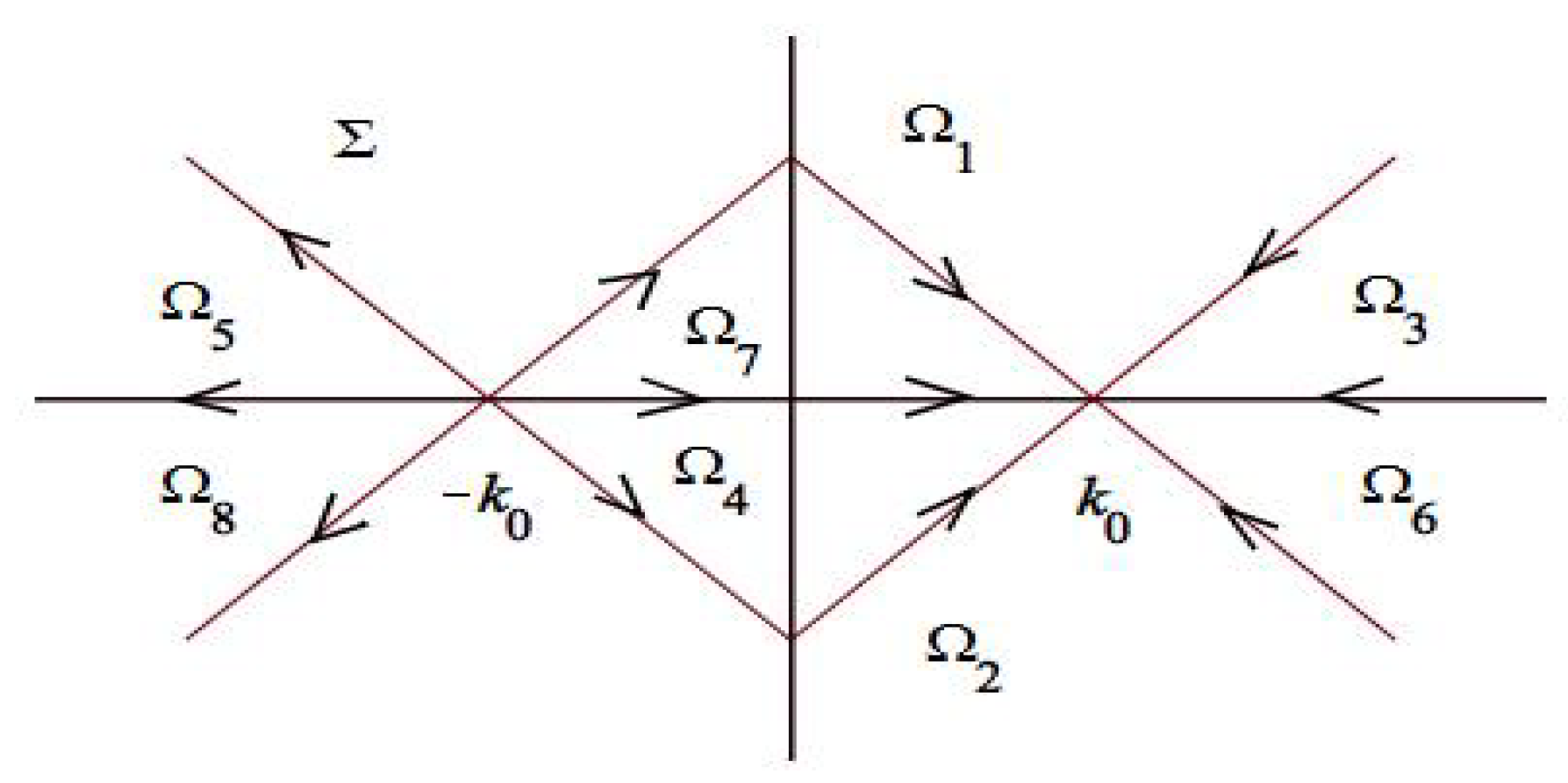
Let be the truncated contour with the orientation as in Figure 8. We will reduce the RH problem (148) from to , and estimate the difference between the two RH problems, one on and the other on .
Let be a sum of three terms
where is supported on and is composed of the contributions to from terms of type and , is supported on and is composed of terms of type and , and is supported on and is composed of terms of type and .
Define
Obviously on , and hence is supported on from terms of type and .
Lemma 1.
For sufficiently small ε, we have
where .
Proof.
The estimates (158), (159) and (160) can be derived, similarly to Proposition 1. Based on the early definition of , we can see that
on the contour , where . On this contour, by (110), we have
and then using (72), we find that
It then follows from a direct computation that the estimate (161) holds. □
Similarly to Proposition 2.23 in [7], we can show the following estimate.
Proposition 2.
In the physically interesting region , as , there exists the inverse of the operator , which is uniformly bounded:
Corollary 1.
In the physically interesting region , as , there exists the inverse of the operator , which is uniformly bounded:
Proof.
Noting , we have
In addition, it follows from Lemma 1 that
in the physically interesting region (where is bounded and thus ). Therefore, we have
Now first from we know, based on (164), that exists.
Second, the second resolvent identity tells
Again based on (164), we see from this identity that the estimate in the corollary is just a consequence of Proposition 2. □
Theorem 4.
As , we have
Proof.
Note that as , we can reduce from to , and for simplicity’s sake, we still denote this reduced operator by . Then
and thus it follows from Theorems 3 and 4 that the following statement holds.
Theorem 5.
As , we have
Let , which yields , and denote . Then, we see that
solves the following RH problem
where the jump matrix is defined by
4.5. Disconnecting Contour Components
Denote the contour (see Figure 8), and set
where
Further define
and thus
The two Cauchy operators and (see (150) for definition) are bounded operators from .
One can prove a similar lemma to Lemma 3.5 in [7].
Lemma 2.
We have the estimates
and
Proposition 3.
As , we have
Proof.
From the identity
it follows that
which implies that
In the above computation, we denote
for simplicity’s sake. Note that if an operator T is bounded and the inverse of exists, then is also bounded. Further, based on the two Lemmas, Lemmas 1 and 2, and one proposition, Proposition 2, we can derive the estimate (179). □
Now, from Theorem 5 and Proposition 3, we see that the following result holds.
Theorem 6.
As , we have
4.6. Rescaling and Reduction of the Disconnected RH Problem
Extend the two contours and to the following two contours
and define on as
respectively, where
Let and denote the contours
oriented outward as in and inward as in , respectively (see Figure 9).
Motivated by the method of stationary phase, define the scaling transformations
and denote
A direct change-of-variable argument tells that
where (or ) is a bounded operator from (or into (or ). On the part
of the contour , we have
and on the conjugate part , we have
where
Lemma 3.
As , we have the estimates
where , and
where .
Proof.
We only prove the estimate (193) and the proof of the other estimate is completely similar.
From (65) and (66), we see that solves the following RH problem
where
The solution of this vector RH problem is given by
with
Noting that
we can have when , upon noting the definition of , and decompose into two parts: , where satisfies
and has an analytical continuation from to (see Figure 10):
and satisfies
Let , and we decompose
As , for the first and second terms, we can have
which are due to and
respectively. By using Cauchy’s Theorem, we can have a similar estimate through integrating along the contour in instead of the interval on . Now, the estimate (193) is a consequence of those three estimates. The proof is finished. □
Express
where
with
Based on (193), (194) and Lemma 3.35 in [7], we can obtain
Therefore, we have
Together with a similar argument for B, we can obtain
For , we set
which solves the following RH problem
Particularly, from an asymptotic expansion
we get
4.7. The Model RH Problem and Its Solution
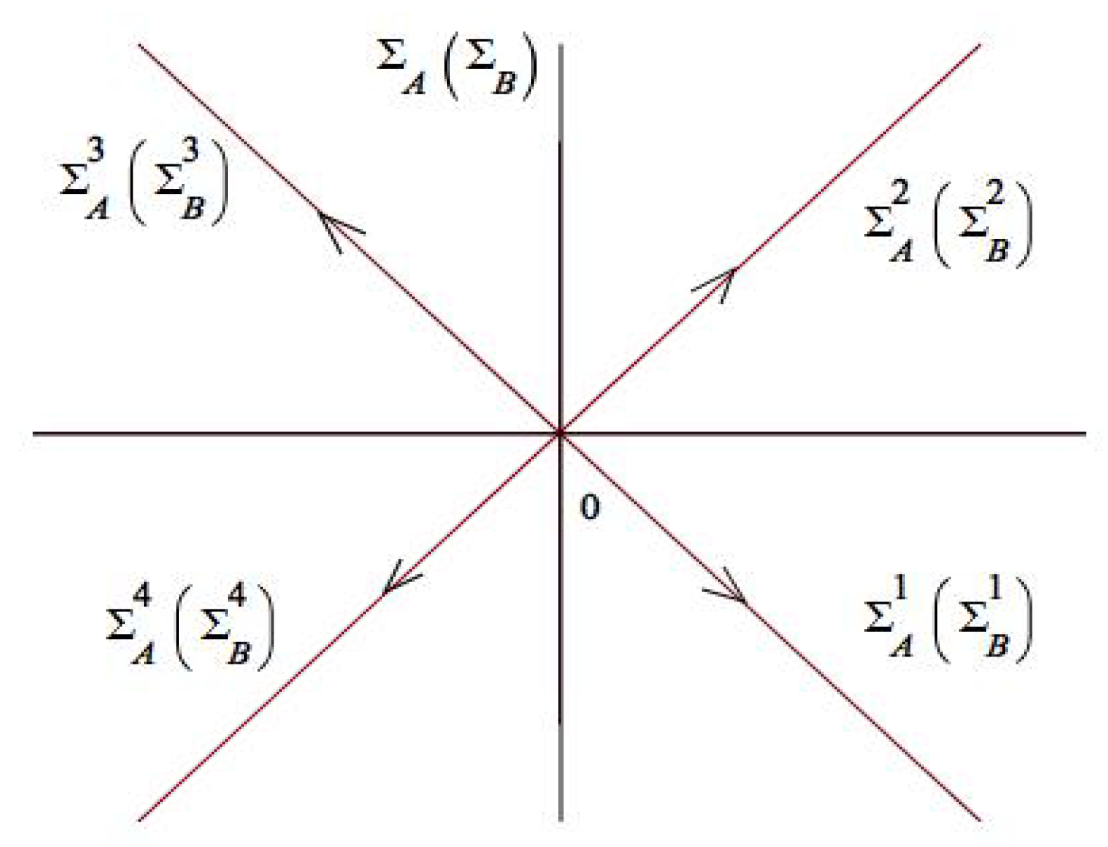
To determine explicitly, we solve a model RH problem
The solution to this RH problem is given by
where and .
Since the jump matrix does not depend on k along each ray of , we have
Together with (216), this implies that has no jump discontinuity along any of the four rays. Directly from the solution, we obtain
It then follows from Liouville’s theorem that
where
Particularly, we have
We partition into the following form
where is a scalar and is a matrix. From the differential Equation (219) for , we obtain
where
provided that (note that the case of is, of course, trivial).
As is well known, the following Weber’s equation
has a general solution
where are arbitrary constants and denotes the standard (entire) parabolic-cylinder function which satisfies
being the Gamma function. From the textbook [54] (see pp. 347–349), we know that as ,
Denote and then
Thus we find
where and are constants, and and are row vectors of constants. Note that as and ,
Thus, for , we have
and further,
For , we have
and further,
5. Concluding Remarks
The paper is dedicated to determination of long-time asymptotics of the three-component coupled mKdV system, based on an associated Riemann-Hilbert (RH) problem. The crucial step is to deform the associated RH problem to the one which is solvable explicitly, and estimate small errors between solutions to different deformed RH problems. This is an example of applications of the nonlinear steepest descent method to asymptotics in the case of matrix spectral problems.
The nonlinear steepest descent method is powerful in exploring long-time asymptotics for integrable systems and even nonlocal integrable systems (see also, e.g., [55]). Moreover, it has been generalized to determine asymptotics of initial-boundary value problems of integrable systems on the half-line (see, e.g., [56,57,58]), and asymptotics of integrable systems whose RH problems possess rational phases (see, e.g., [16]) or non-analytic jumps (see, e.g., [19]).
There are various other approaches in the field of integrable systems, which include the Hirota direct method [59], the generalized bilinear technique [60], the Wronskian technique [61,62] and the Darboux transformation [63]. Connections between different approaches would be interesting. About coupled mKdV equations, there are many other studies such as integrable couplings [64], super hierarchies [65] and fractional analogous equations [66,67], and an important topic for further study is long-time asymptotics of those generalized integrable counterparts via the nonlinear steepest descent method. It is hoped that our result could be helpful in computing limiting behaviors of solutions incorporating features of other exact solutions, such as lumps [68,69], from the perspective of steepest descent based on RH problems.
Funding
This research was in part funded by NSFC under the grants 11371326, 11301331 and 11371086, and NSF under the grant DMS-1664561.
Acknowledgments
The author would also like to thank Ahmed A., Adjiri A., Gu X., Hao X.Z., McAnally M., Wang F.D., Wang H., and Zhou Y. for their valuable discussions.
Conflicts of Interest
The author declares no conflict of interest.
References
- Manakov, S.V. Nonlinear Fraunnhofer diffraction. Sov. Phys. JETP 1974, 38, 693–696. [Google Scholar]
- Ablowitz, M.J.; Newell, A.C. The decay of the continuous spectrum for solutions of the Korteweg-de Vries equation. J. Math. Phys. 1973, 14, 1277–1284. [Google Scholar] [CrossRef]
- Zakharov, V.E.; Manakov, S.V. Asymptotic behavior of non-linear wave systems integrated by the inverse scattering method. Sov. Phys. JETP 1976, 44, 106–112. [Google Scholar]
- Ablowitz, M.J.; Segur, H. Asymptotic solutions of the Korteweg-de Vries equation. Stud. Appl. Math. 1977, 57, 13–44. [Google Scholar] [CrossRef]
- Segur, H.; Ablowitz, M.J. Asymptotic solutions and conservation laws for the nonlinear Schrödinger equation I. J. Math. Phys. 1973, 17, 710–713. [Google Scholar] [CrossRef]
- Its, A.R. Asymptotics of solutions of the nonlinear Schrödinger equation and isomonodromic deformations of systems of linear differential equations. Sov. Math. Dokl. 1981, 24, 452–456. [Google Scholar]
- Deift, P.; Zhou, X. A steepest descent method for oscillatory Riemann-Hilbert problems: Asymptotics for the MKdV equation. Ann. Math. 1993, 137, 295–368. [Google Scholar] [CrossRef]
- Deift, P.; Venakides, S.; Zhou, X. The collisionless shock region for the long-time behavior of solutions of the KdV equation. Commun. Pure Appl. Math. 1994, 47, 199–206. [Google Scholar] [CrossRef]
- Deift, P.; Zhou, X. Asymptotics for the Painlevé II equation. Commun. Pure Appl. Math. 1995, 48, 277–337. [Google Scholar] [CrossRef]
- Deift, P.; Venakides, S.; Zhou, X. New results in small dispersion KdV by an extension of the steepest descent method for Riemann-Hilbert problems. Int. Math. Res. Not. 1997, 1997, 286–299. [Google Scholar] [CrossRef]
- Kamvissis, S. Long time behavior for the focusing nonlinear Schroedinger equation with real spectral singularities. Commun. Math. Phys. 1996, 180, 325–341. [Google Scholar] [CrossRef]
- Kitaev, A.V.; Vartanian, A.H. Leading-order temporal asymptotics of the modified nonlinear Schrödinger equation: Solitonless sector. Inverse Probl. 1997, 13, 1311–1339. [Google Scholar] [CrossRef]
- Cheng, P.J.; Venakides, S.; Zhou, X. Long-time asymptotics for the pure radiation solution of the sine-Gordon equation. Commun. Part. Differ. Equ. 1999, 24, 1195–1262. [Google Scholar] [CrossRef]
- Grunert, K.; Teschl, G. Long-time asymptotics for the Korteweg-de Vries equation via nonlinear steepest descent. Math. Phys. Anal. Geom. 2009, 12, 287–324. [Google Scholar] [CrossRef]
- Boutet de Monvel, A.; Kostenko, A.; Shepelsky, D.; Teschl, G. Long-time asymptotics for the Camassa-Holm equation. SIAM J. Math. Anal. 2009, 41, 1559–1588. [Google Scholar] [CrossRef]
- Xu, J.; Fan, E.G. Long-time asymptotics for the Fokas-Lenells equation with decaying initial value problem: Without solitons. J. Differ. Equ. 2015, 259, 1098–1148. [Google Scholar] [CrossRef]
- Andreiev, K.; Egorova, I.; Lange, T.L.; Teschl, G. Rarefaction waves of the Korteweg-de Vries equation via nonlinear steepest descent. J. Differ. Equ. 2016, 261, 5371–5410. [Google Scholar] [CrossRef]
- Wang, D.S.; Wang, X.L. Long-time asymptotics and the bright N-soliton solutions of the Kundu-Eckhaus equation via the Riemann-Hilbert approach. Nonlinear Anal. Real World Appl. 2018, 41, 334–361. [Google Scholar] [CrossRef]
- McLaughlin, K.T.-R.; Miller, P.D. The ∂¯ steepest descent method and the asymptotic behavior of polynomials orthogonal on the unit circle with fixed and exponentially varying nonanalytic weights. Int. Math. Res. Pap. 2006, 2006, 1–77. [Google Scholar] [CrossRef]
- Varzugin, G.G. Asymptotics of oscillatory Riemann-Hilbert problems. J. Math. Phys. 1996, 37, 5869–5892. [Google Scholar] [CrossRef]
- Geng, X.G.; Xue, B. Quasi-periodic solutions of mixed AKNS equations. Nonlinear Anal. Theory Meth. Appl. 2010, 73, 3662–3674. [Google Scholar] [CrossRef]
- Boutet de Monvel, A.; Shepelsky, D. A Riemann-Hilbert approach for the Degasperis-Procesi equation. Nonlinearity 2013, 26, 2081–2107. [Google Scholar] [CrossRef]
- Geng, X.G.; Liu, H. The nonlinear steepest descent method to long-time asymptotics of the coupled nonlinear Schrödinger equation. J. Nonlinear Sci. 2018, 28, 739–763. [Google Scholar] [CrossRef]
- Wu, J.P.; Geng, X.G. Inverse scattering transform and soliton classification of the coupled modified Korteweg-de Vries equation. Commun. Nonlinear Sci. Numer. Simul. 2017, 53, 83–93. [Google Scholar] [CrossRef]
- Ma, W.X. The inverse scattering transform and soliton solutions of a combined modified Korteweg-de Vries equation. J. Math. Anal. Appl. 2019, 471, 796–811. [Google Scholar] [CrossRef]
- Ma, W.X. Trigonal curves and algebro-geometric solutions to soliton hierarchies I. Proc. R. Soc. A 2017, 473, 20170232. [Google Scholar] [CrossRef] [PubMed]
- Ma, W.X. Trigonal curves and algebro-geometric solutions to soliton hierarchies II. Proc. R. Soc. A 2017, 473, 20170233. [Google Scholar] [CrossRef] [PubMed] [Green Version]
- Ma, W.X. Binary Bargmann symmetry constraints of soliton equations. Nonlinear Anal. Theory Meth. Appl. 2001, 47, 5199–5211. [Google Scholar] [CrossRef] [Green Version]
- Ma, W.X. Riemann-Hilbert problems of a six-component mKdV system and its soliton solutions. Acta Math. Sci. 2019, 39, 509–523. [Google Scholar]
- Ma, W.X.; Zhou, Z.X. Binary symmetry constraints of N-wave interaction equations in 1+1 and 2+1 dimensions. J. Math. Phys. 2001, 42, 4345–4382. [Google Scholar] [CrossRef] [Green Version]
- Tu, G.Z. On Liouville integrability of zero-curvature equations and the Yang hierarchy. J. Phys. A Math. Gen. 1989, 22, 2375–2392. [Google Scholar]
- Lax, P.D. Integrals of nonlinear equations of evolution and solitary waves. Commun. Pure Appl. Math. 1968, 21, 467–490. [Google Scholar] [CrossRef]
- Magri, F. A simple model of the integrable Hamiltonian equation. J. Math. Phys. 1978, 19, 1156–1162. [Google Scholar] [CrossRef]
- Ma, W.X.; Chen, M. Hamiltonian and quasi-Hamiltonian structures associated with semi-direct sums of Lie algebras. J. Phys. A Math. Gen. 2006, 39, 10787–10801. [Google Scholar] [CrossRef] [Green Version]
- Ma, W.X. Variational identities and applications to Hamiltonian structures of soliton equations. Nonlinear Anal. Theor. Meth. Appl. 2009, 71, e1716–e1726. [Google Scholar] [CrossRef]
- Ma, W.X. Generators of vector fields and time dependent symmetries of evolution equations. Sci. China A 1991, 34, 769–782. [Google Scholar]
- Ma, W.X. The algebraic structure of zero curvature representations and application to coupled KdV systems. J. Phys. A Math. Gen. 1993, 26, 2573–2582. [Google Scholar] [CrossRef]
- Ma, W.X.; Zhou, R.G. Adjoint symmetry constraints leading to binary nonlinearization. J. Nonlinear Math. Phys. 2002, 9 (Suppl. 1), 106–126. [Google Scholar] [CrossRef]
- Ma, W.X. Conservation laws by symmetries and adjoint symmetries. Discrete Contin. Dyn. Syst. S 2018, 11, 707–721. [Google Scholar] [CrossRef]
- Drinfel’d, V.G.; Sokolov, V.V. Equations of Korteweg-de Vries type, and simple Lie algebras. Sov. Math. Dokl. 1982, 23, 457–462. [Google Scholar]
- Terng, C.L.; Uhlenbeck, K. The n × n KdV hierarchy. J. Fixed Point Theory Appl. 2011, 10, 37–61. [Google Scholar] [CrossRef]
- Ma, W.X.; Xu, X.X.; Zhang, Y.F. Semi-direct sums of Lie algebras and continuous integrable couplings. Phys. Lett. A 2006, 351, 125–130. [Google Scholar] [CrossRef] [Green Version]
- Manakov, S.V. On the theory of two-dimensional stationary self-focusing of electromagnetic waves. Sov. Phys. JETP 1974, 38, 248–253. [Google Scholar]
- Chen, S.T.; Zhou, R.G. An integrable decomposition of the Manakov equation. Comput. Appl. Math. 2012, 31, 1–18. [Google Scholar]
- Ma, W.X. Symmetry constraint of MKdV equations by binary nonlinearization. Physica A 1995, 219, 467–481. [Google Scholar] [CrossRef] [Green Version]
- Yu, J.; Zhou, R.G. Two kinds of new integrable decompositions of the mKdV equation. Phys. Lett. A 2006, 349, 452–461. [Google Scholar] [CrossRef]
- Ma, W.X.; Yong, X.L.; Qin, Z.Y.; Gu, X.; Zhou, Y. A generalized Liouville’s formula. Appl. Math. B-A J. Chin. Univ. 2016. submitted. [Google Scholar]
- Novikov, S.P.; Manakov, S.V.; Pitaevskii, L.P.; Zakharov, V.E. Theory of Solitons: The Inverse Scattering Method; Consultants Bureau: New York, NY, USA, 1984. [Google Scholar]
- Ma, W.X. Application of the Riemann-Hilbert approach to the multicomponent AKNS integrable hierarchies. Nonlinear Anal. Real World Appl. 2019, 47, 1–17. [Google Scholar] [CrossRef]
- Zhou, X. The Riemann-Hilbert problem and inverse scattering. SIAM J. Math. Anal. 1989, 20, 966–986. [Google Scholar] [CrossRef]
- Ablowitz, M.J.; Fokas, A.S. Complex Variables: Introduction and Applications; Cambridge University Press: Cambridge, UK, 2003. [Google Scholar]
- Beals, R.; Coifman, R.R. Scattering and inverse scattering for first order systems. Commun. Pure Appl. Math. 1984, 37, 39–90. [Google Scholar] [CrossRef]
- Clancey, K.; Gohberg, I. Factorization of Matrix Functions and Singular Integral Operators; Birkhäuser: Basel, Switzerland, 1981. [Google Scholar]
- Whittaker, E.T.; Watson, G.N. A Course of Modern Analysis, 4th ed.; Cambridge University Press: Cambridge, UK, 1927. [Google Scholar]
- Rybalko, Y.; Shepelsky, D. Long-time asymptotics for the integrable nonlocal nonlinear Schrödinger equation. J. Math. Phys. 2019, 60, 031504. [Google Scholar] [CrossRef]
- Boutet de Monvel, A.; Fokas, A.S.; Shepelsky, D. The mKdV equation on the half-line. J. Inst. Math. Jussieu 2004, 3, 139–164. [Google Scholar] [CrossRef]
- Lenells, J. The nonlinear steepest descent method: Asymptotics for initial-boundary value problems. SIAM J. Math. Anal. 2016, 48, 2076–2118. [Google Scholar] [CrossRef]
- Guo, B.L.; Liu, N. Long-time asymptotics for the Kundu-Eckhaus equation on the half-line. J. Math. Phys. 2018, 59, 061505. [Google Scholar] [CrossRef]
- Hirota, R. The Direct Method in Soliton Theory; Cambridge University Press: New York, NY, USA, 2004. [Google Scholar]
- Ma, W.X. Generalized bilinear differential equations. Stud. Nonlinear Sci. 2011, 2, 140–144. [Google Scholar]
- Freeman, N.C.; Nimmo, J.J.C. Soliton solutions of the Korteweg-de Vries and Kadomtsev-Petviashvili equations: The Wronskian technique. Phys. Lett. A 1983, 95, 1–3. [Google Scholar] [CrossRef]
- Ma, W.X.; You, Y. Solving the Korteweg-de Vries equation by its bilinear form: Wronskian solutions. Trans. Am. Math. Soc. 2005, 357, 1753–1778. [Google Scholar] [CrossRef]
- Matveev, V.B.; Salle, M.A. Darboux Transformations and Solitons; Springer: Berlin, Germany, 1991. [Google Scholar]
- Xu, X.X. An integrable coupling hierarchy of the MKdV_ integrable systems, its Hamiltonian structure and corresponding nonisospectral integrable hierarchy. Appl. Math. Comput. 2010, 216, 344–353. [Google Scholar]
- Dong, H.H.; Zhao, K.; Yang, H.W.; Li, Y.Q. Generalised (2+1)-dimensional super MKdV hierarchy for integrable systems in soliton theory. East Asian J. Appl. Math. 2015, 5, 256–272. [Google Scholar] [CrossRef]
- Dong, H.H.; Guo, B.Y.; Yin, B.S. Generalized fractional supertrace identity for Hamiltonian structure of NLS-MKdV hierarchy with self-consistent sources. Anal. Math. Phys. 2016, 6, 199–209. [Google Scholar] [CrossRef]
- Guo, M.; Fu, C.; Zhang, Y.; Liu, J.X.; Yang, H.W. Study of ion-acoustic solitary waves in a magnetized plasma using the three-dimensional time-space fractional Schamel-KdV equation. Complexity 2018, 2018, 6852548. [Google Scholar] [CrossRef]
- Ma, W.X.; Zhou, Y. Lump solutions to nonlinear partial differential equations via Hirota bilinear forms. J. Differ. Equ. 2018, 264, 2633–2659. [Google Scholar] [CrossRef]
- Ma, W.X.; Li, J.; Khalique, C.M. A study on lump solutions to a generalized Hirota-Satsuma-Ito equation in (2+1)-dimensions. Complexity 2018, 2018, 9059858. [Google Scholar] [CrossRef]
Figure 1.
Increasing and decreasing of .

Figure 2.
The signature table of when .

Figure 3.
The oriented contour on .

Figure 4.
The oriented jump contour .

Figure 5.
Part of in the upper half k-plane.
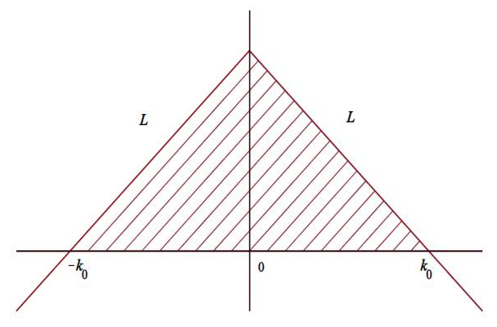
Figure 6.
Part of in the lower half k-plane.

Figure 7.
Deformation of a RH problem.

Figure 8.
The oriented contour .
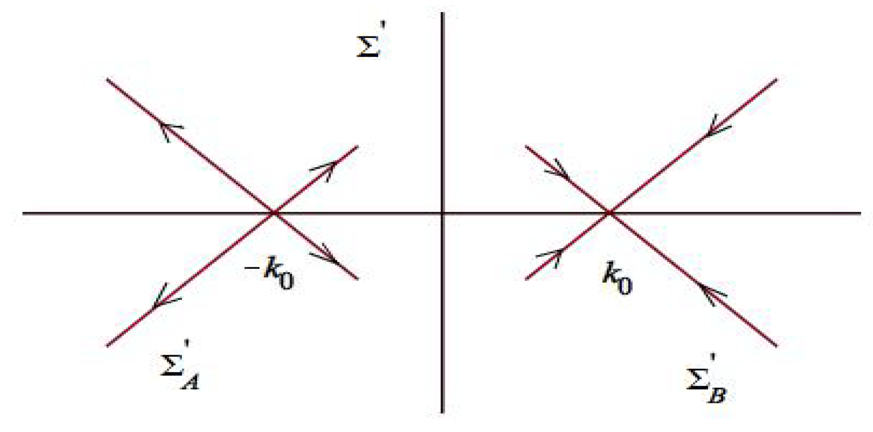
Figure 9.
Oriented contours and (reoriented).

Figure 10.
The oriented contour .
© 2019 by the author. Licensee MDPI, Basel, Switzerland. This article is an open access article distributed under the terms and conditions of the Creative Commons Attribution (CC BY) license (http://creativecommons.org/licenses/by/4.0/).
Share and Cite
MDPI and ACS Style
Ma, W.-X. Long-Time Asymptotics of a Three-Component Coupled mKdV System. Mathematics 2019, 7, 573. https://doi.org/10.3390/math7070573
AMA Style
Ma W-X. Long-Time Asymptotics of a Three-Component Coupled mKdV System. Mathematics. 2019; 7(7):573. https://doi.org/10.3390/math7070573
Chicago/Turabian StyleMa, Wen-Xiu. 2019. "Long-Time Asymptotics of a Three-Component Coupled mKdV System" Mathematics 7, no. 7: 573. https://doi.org/10.3390/math7070573
Note that from the first issue of 2016, this journal uses article numbers instead of page numbers. See further details here.