Pricing Decision within an Inventory Model for Complementary and Substitutable Products


Abstract
1. Introduction
2. Literature Review
3. Problem Description, Notation, and Assumptions
3.1. Problem Definition
3.2. Notation
3.3. Assumptions
- A retailer maximizes the profit based on an economic order quantity (EOQ) model. The demand is dependent upon selling prices and lot sizes of two types of products. The demand of two complementary products is dependent upon each product’s selling price and the degree of complementarity.
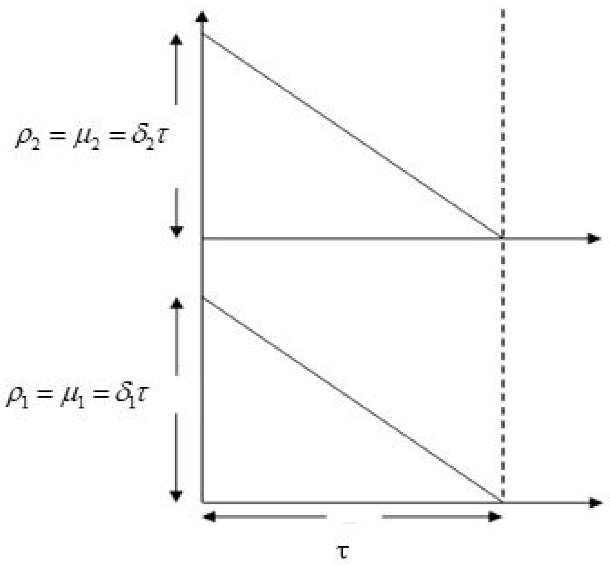
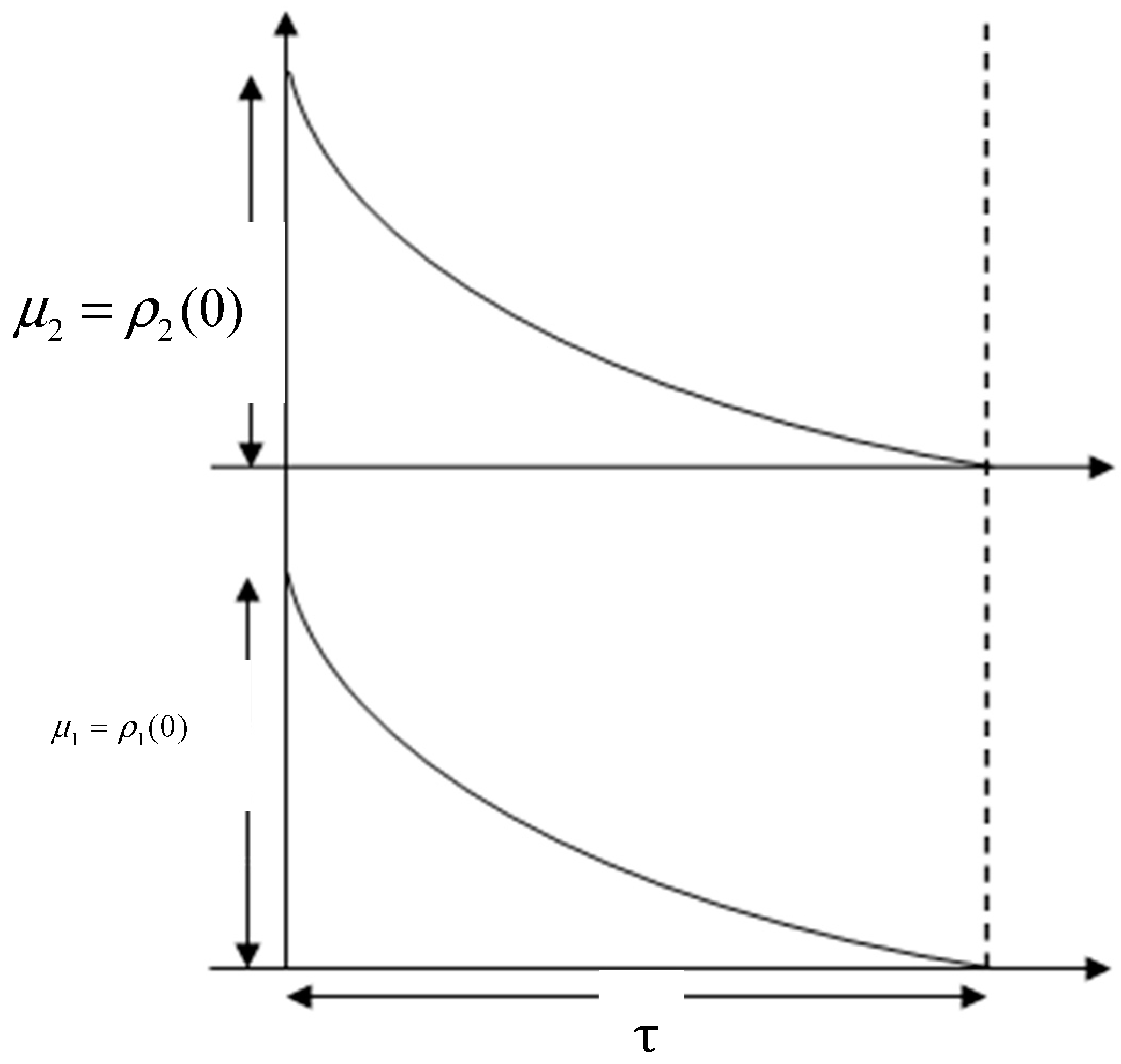
- After a certain time, products start to deteriorate with a constant deterioration rate. As deterioration is considered in this model, deterioration cost per time unit for the product m is ($ per unit). The deterioration rate of product 1 and product 2 is .
- The degree of complementarity between two products is given by , where and the degree of substitutability between two products is given by d, where .
- The lead time is zero, and there are no shortages for both types of products.
- The time horizon is infinite.
4. Mathematical Model
4.1. Non-Deteriorating Complementary Products
- Step 1.
- Using Equations (10)–(12), calculate the coefficients of polynomial shown in Equation (9).
- Step 2.
- All positive real roots of Equation (9) are found by using MATLAB software. Go to the Step (3).
- Step 3.
- Determine the values from Step (2).
- Step 4.
- For all combinations of , obtain the profit and check the concavity clause (Theorem 1). Select the maximum value as an optimal value of the profit. Then the related optimum decision variables are , and .
- Step 5.
- Determine the optimal values of the order quantities using and .
4.2. Non-Deteriorating Substitutable Products
- Step 1.
- Using Equations (23)–(25), calculate the coefficients of the polynomial in Equation (22).
- Step 2.
- After finding all possible roots of Equation (22) with the help of MATLAB software, go to the Step (3).
- Step 3.
- From Step 2, determine the values of .
- Step 4.
- For all values of , determine the total profit and check the concavity clause (Theorem 2). Then select the maximum value as the optimum one. The related decision variables associated with the maximum profit are , and .
- Step 5.
- Determine optimal values of order quantities using and .
4.3. Deteriorating Complementary Products
- Step 1.
- Using Equations (38)–(40), calculate coefficients of polynomial shown in the Equation (37).
- Step 2.
- Equation (37) gives all roots by using MATLAB software and then go to the Step (3).
- Step 3.
- Determine all values of for period from the Step (2).
- Step 4.
- For all possible combinations of , determine the total profit and check the concavity clause (Theorem 3). Select the maximum value as the optimal value of the profit. Then optimal values of the decision variables are , and .
4.4. Deteriorating Substitutable Products
- Step 1.
- Calculate the coefficients of polynomial from the Equation (49) by using Equations (50) to (52).
- Step 2.
- Equation (49) gives the roots of the equation using MATLAB software. Move to the Step 3.
- Step 3.
- Find using Step 2.
- Step 4.
- For , obtain the profit and check the concavity clause (Theorem4). Choose the maximum value as the optimal value of the profit. Then related decision variables for the maximum profit are given by , and .
- Step 5.
- Determine optimal values of order quantities using and .
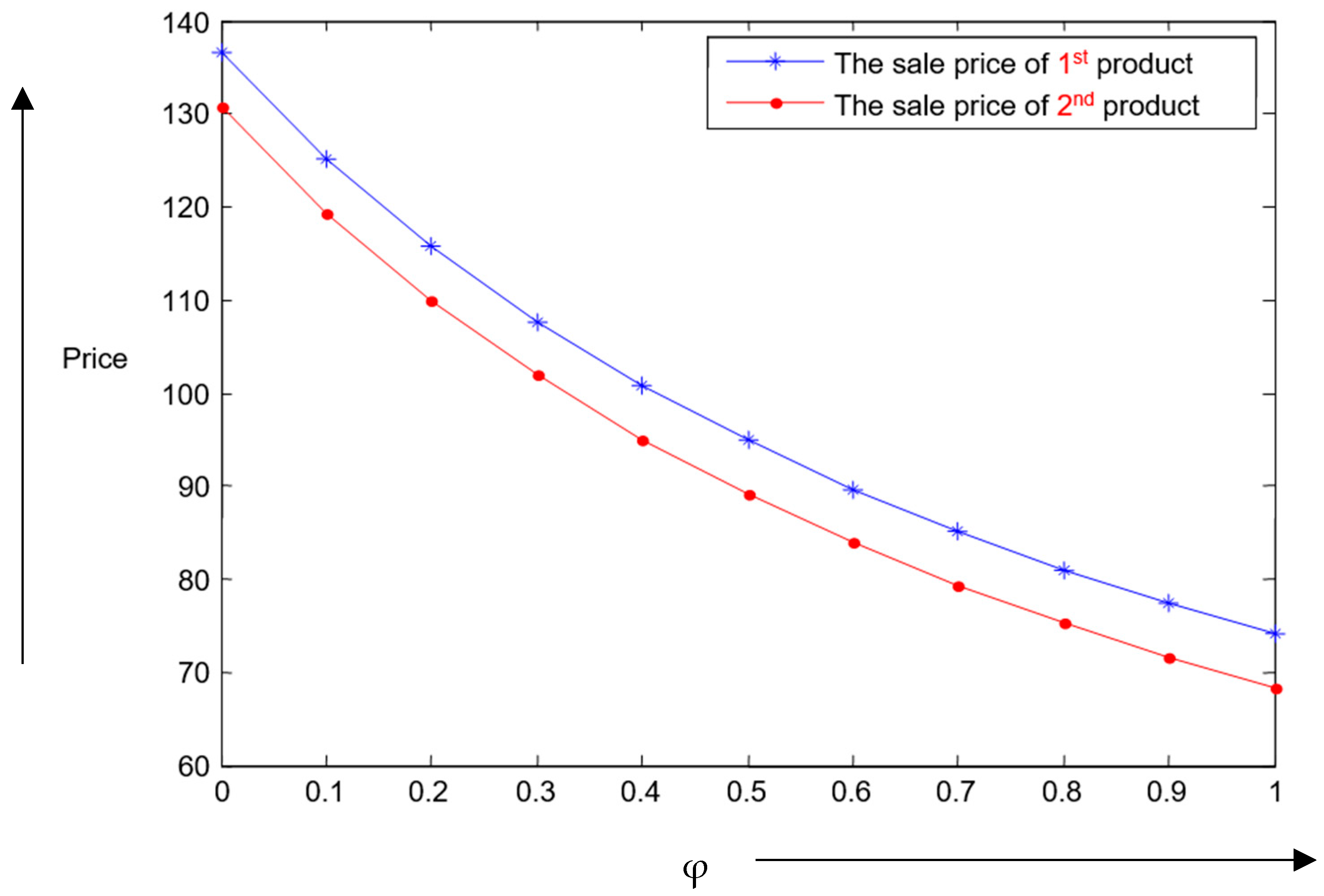
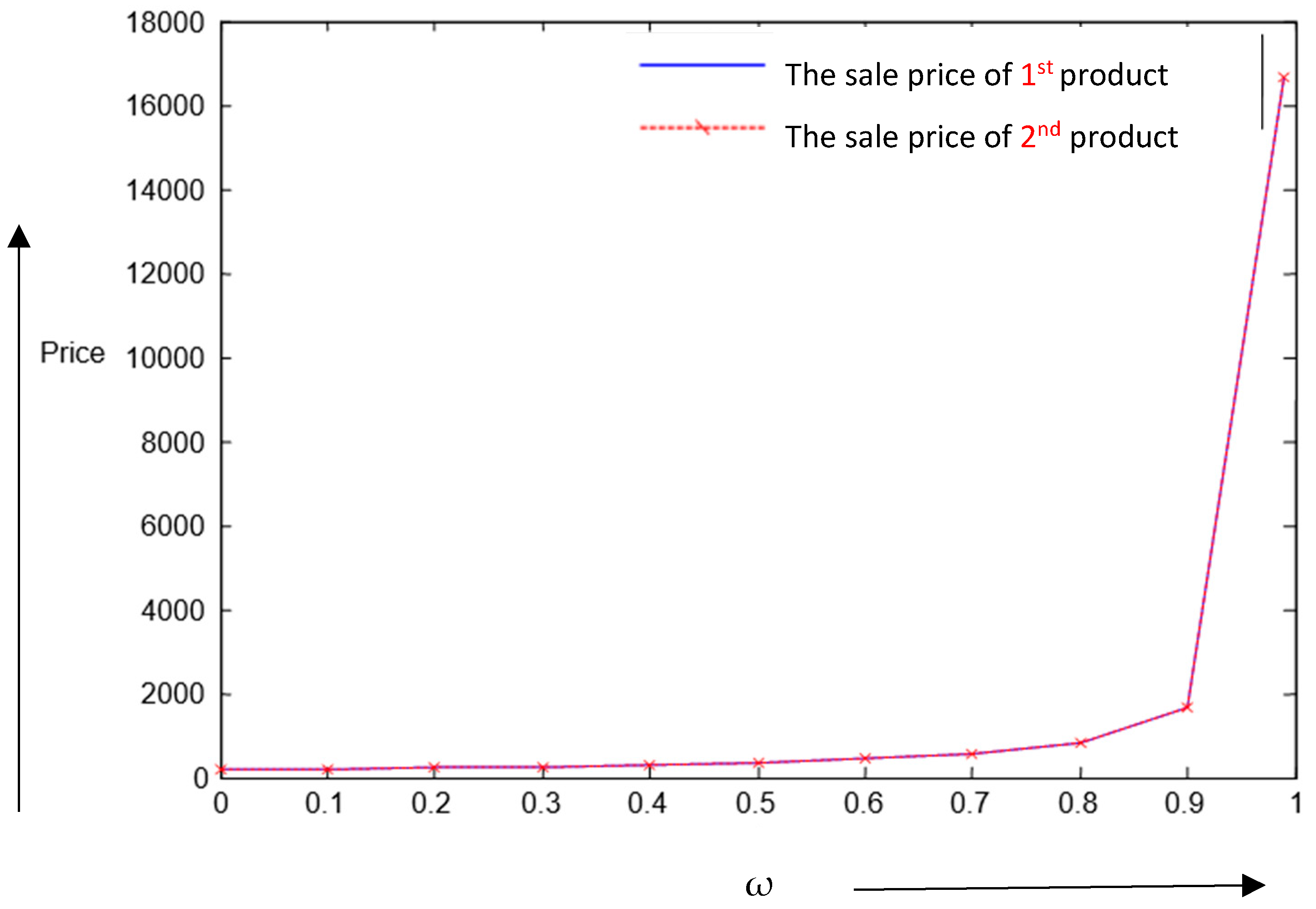
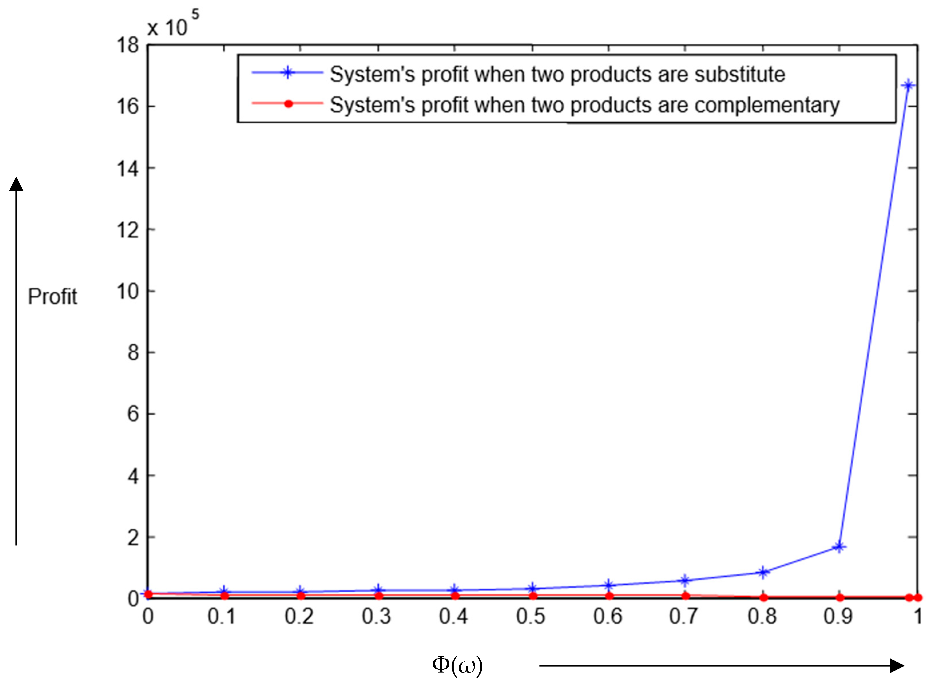
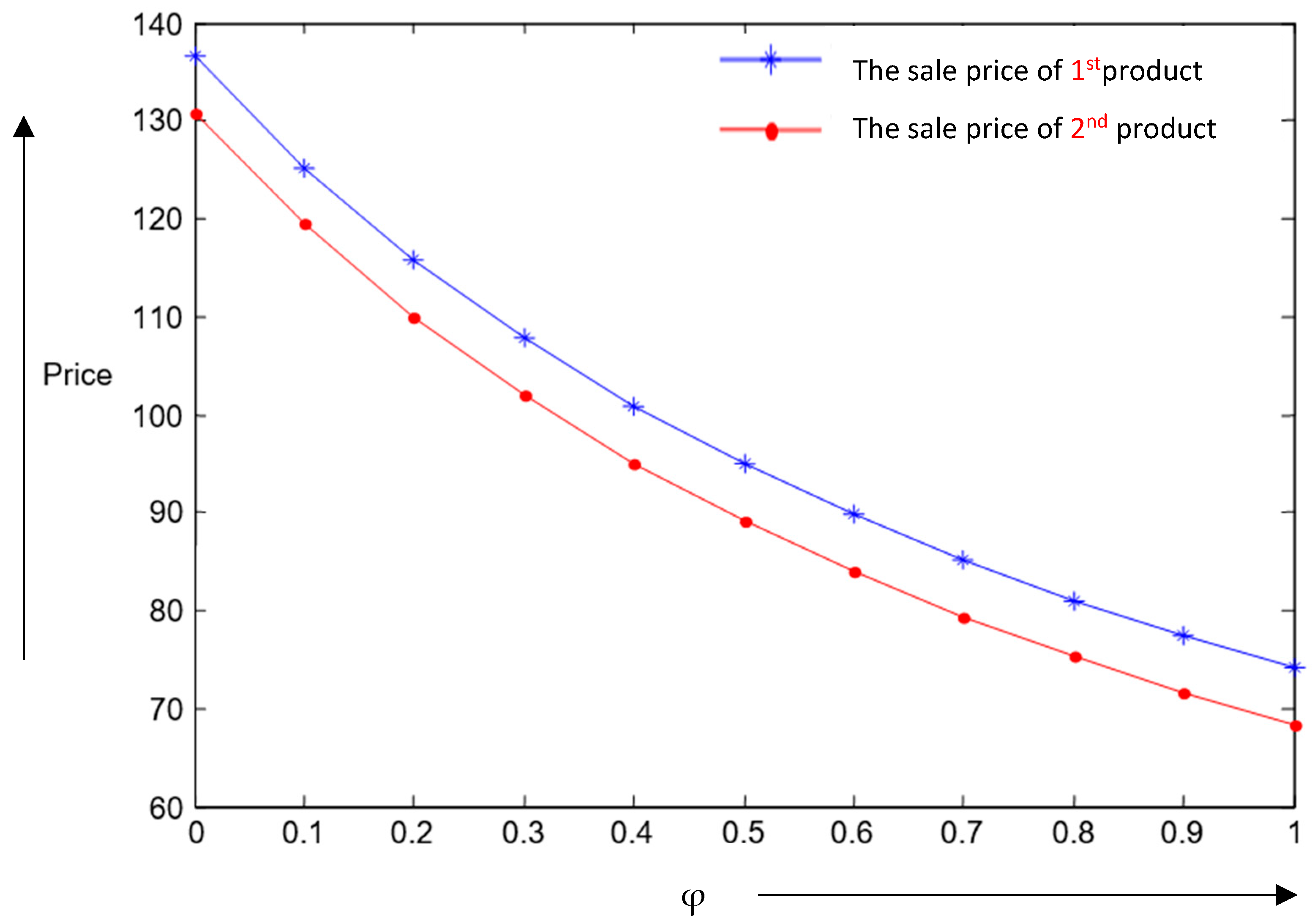
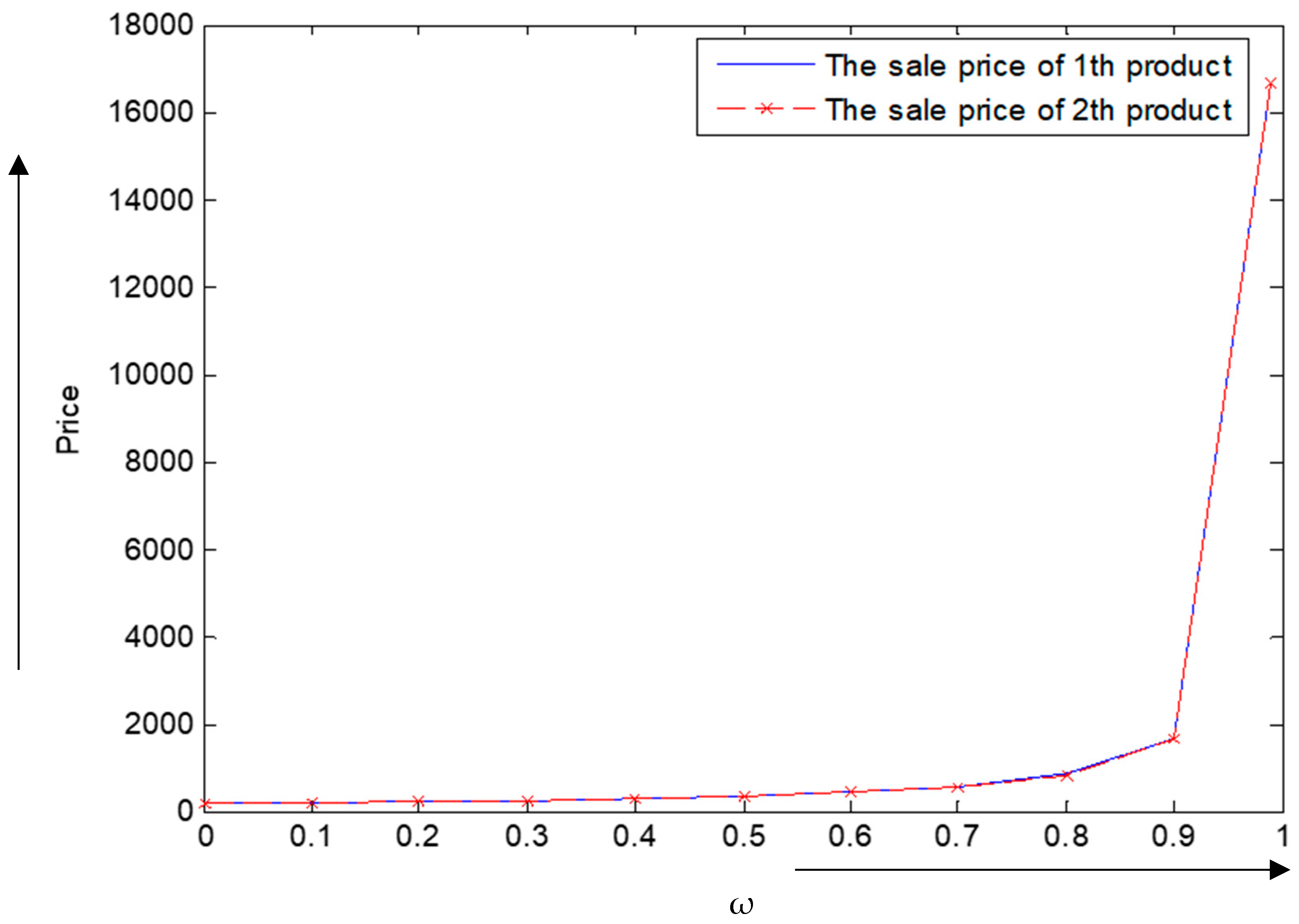
5. Numerical Examples and Sensitivity Analysis
5.1. Example 1: Non-Deteriorating Complementary Products
5.2. Example 2: Non-Deteriorating Substitutable Products
5.3. Example 3: Deteriorating Complementary Products
5.4. Example 4: Deteriorating Substitutable Products
Managerial insights
6. Conclusions
Author Contributions
Funding
Conflicts of Interest
Nomenclature
| Index | Description |
| 1, 2 | |
| Decision variables | |
| product ’s selling price ($/unit) | |
| order quantity of product (units) | |
| τ | time interval between two replenishments |
| Parameters | |
| market demand for product 1 (units) | |
| demand for product 2 (units) | |
| inventory level at time τ of product m | |
| ∝ | basic potential demand (units) |
| 𝛽 | self-price sensitivity |
| holding cost of product m ($/unit/unit time) | |
| purchasing cost of product m ($/unit) | |
| deterioration cost of product m ($/unit) | |
| deterioration rate of product 1 and product 2 | |
| degree of complementarity of two products, | |
| 𝜔 | degree of substitutability of two products, |
Appendix A
Appendix B
Appendix C
Appendix D
References
- Shocker, A.D.; Bayus, B.L.; Kim, N. Product complments and substitutes in the real world: The relevence of “other products”. J. Market. 2004, 68, 28–40. [Google Scholar] [CrossRef]
- Sarkar, M.; Lee, Y.H. Optimum pricing strategy for complementary products with stochastic reservation price in a supply chain model. J. Ind. Manag. Optim. 2017, 13, 1553–1586. [Google Scholar]
- Avgeropoulos, S.; Sammut-Bonnici, T.; McGee, J. Complementary products. Encycl. Manag. 2015, 12. [Google Scholar] [CrossRef]
- Sana, S.S. Price-sensitive demand for perishable items—An EOQ model. Appl. Math. Comput. 2011, 217, 6248–6259. [Google Scholar]
- Sarkar, B.; Saren, S.; Wee, H.M. An inventory model with variable demand, component cost and selling price for deteriorating items. Econ. Model. 2013, 30, 306–310. [Google Scholar] [CrossRef]
- Salvietti, L.; Smith, N.R.; Cárdenas-Barrón, L.E. A stochastic profit-maximising economic lot scheduling problem with price optimisation. Eur. J. Oper. Res. 2014, 8, 193–221. [Google Scholar] [CrossRef]
- Smith, N.R.; Robles, J.L.; Cárdenas-Barrón, L.E. Optimal pricing and production master planning in a multiperiod horizon considering capacity and inventory constraints. Math. Probl. Eng. 2009, 932676, 15. [Google Scholar] [CrossRef]
- Soon, W. A review of multi-product pricing models. Appl. Math. Comput. 2011, 217, 8149–8165. [Google Scholar] [CrossRef]
- Wei, J.; Zhao, J.; Li, Y. Pricing decisions for complementary products with firms’ different market powers. Eur. J. Oper. Res. 2013, 224, 507–519. [Google Scholar] [CrossRef]
- Dey, B.; Sarkar, B.; Sarkar, M.; Pareek, S. An integrated inventory model involving discrete setup cost reduction, variable safety factor, selling-price dependent demand, and investment. RAIRO-Oper. Res. 2019, 53, 39–57. [Google Scholar] [CrossRef]
- Mcgillivray, R.; Silver, E. Some concepts for inventory control under substitutable demand. Inf. Syst. Oper. Res. 1978, 16, 47–63. [Google Scholar] [CrossRef]
- Zhang, R.Q.; Kaku, I.; Xiao, Y.Y. Deterministic EOQ with partial backordering and correlated demand caused by cross-selling. Eur. J. Oper. Res. 2011, 210, 537–551. [Google Scholar] [CrossRef]
- Zhang, R.Q. An extension of partial backordering EOQ with correlated demand caused by cross-selling considering multiple minor items. Eur. J. Oper. Res. 2012, 220, 876–881. [Google Scholar] [CrossRef]
- Yue, X.; Mukhopadhyay, S.K.; Zhu, X. A Bertrand model of pricing of complementary goods under information asymmetry. J. Bus. Res. 2006, 59, 1182–1192. [Google Scholar] [CrossRef]
- Liu, L.; Yuan, X.M. Coordinated replenishments in inventory systems with correlated demands. Eur. J. Oper. Res. 2000, 123, 490–503. [Google Scholar] [CrossRef]
- Guchhait, R.; Sarkar, M.; Sarkar, B.; Pareek, S. Single-vendor multi-buyer game theoretic model under multi-factor dependent demand. Int. J. Inventory Res. 2017, 4, 303–332. [Google Scholar] [CrossRef]
- Shavandi, H.; Mahlooji, H.; Nosratian, N.E. A constrained multi-product pricing and inventory control problem. Appl. Soft Comput. 2012, 12, 2454–2461. [Google Scholar] [CrossRef]
- Abad, P.L. Optimal pricing and lot-sizing under conditions of perishability, finite production and partial backordering and lost sale. Eur. J. Oper. Res. 2003, 144, 677–685. [Google Scholar] [CrossRef]
- Balkhi, Z.T.; Benkherouf, L. On an inventory model for deteriorating items with stock dependent and time-varying demand rates. Comput. Oper. Res. 2004, 31, 223–240. [Google Scholar] [CrossRef]
- Anjos, M.F.; Cheng, R.C.; Currie, C.S. Optimal pricing policies for perishable products. Eur. J. Oper. Res. 2005, 166, 246–254. [Google Scholar] [CrossRef]
- Dye, C.Y. Joint pricing and ordering policy for a deteriorating inventory with partial backlogging. Omega 2007, 35, 184–189. [Google Scholar] [CrossRef]
- Panda, S.; Saha, S.; Basu, M. An EOQ model for perishable products with discounted selling price and stock dependent demand. Cent. Eur. J. Oper. Res. 2009, 17, 31. [Google Scholar] [CrossRef]
- Pang, Z. Optimal dynamic pricing and inventory control with stock deterioration and partial backordering. Oper. Res. Lett. 2011, 39, 375–379. [Google Scholar] [CrossRef]
- Sarkar, B.; Majumder, A.; Sarkar, M.; Dey, B.K.; Roy, G. Two-echelon supply chain model with manufacturing quality improvement and setup cost reduction. J. Ind. Manag. Optim. 2017, 13, 1085–1104. [Google Scholar] [CrossRef]
- Sarkar, B.; Saren, S. Partial trade-credit policy of retailer with exponentially deteriorating items. Int. J. Appl. Comput. Math. 2015, 1, 343–368. [Google Scholar] [CrossRef]
- Sett, B.K.; Sarkar, B.; Sarkar, B.; Yun, W.Y. Optimal replenishment policy with variable deterioration for fixed lifetime products. Sci. Iran. 2016, 23, 2318–2329. [Google Scholar]
- Sarkar, B.; Sett, B.K.; Roy, G.; Goswami, A. Flexible setup cost and deterioration of products in a supply chain model. Int. J. Appl. Comput. Math. 2016, 2, 25–40. [Google Scholar] [CrossRef]
- Sarkar, B.; Mandal, B.; Sarkar, S. Preservation of deteriorating seasonal products with stock-dependent consumption rate and shortages. J. Ind. Manag. Optim. 2017, 13, 187–206. [Google Scholar] [CrossRef]
- Ullah, M.; Sarkar, B.; Asghar, I. Effects of preservation technology investment on waste generation in a two-echelon supply chain model. Mathematics 2019, 7, 20. [Google Scholar] [CrossRef]
- Iqbal, M.W.; Sarkar, B. Recycling of lifetime dependent deteriorated products through different supply chains. RAIRO-Operat. Res. 2019, 53, 129–156. [Google Scholar] [CrossRef]
- Dey, B.K.; Sarkar, B.; Pareek, S. A two-echelon supply chain management with setup time and cost reduction, quality improvement and variable production rate. Mathematics 2019, 7, 25. [Google Scholar] [CrossRef]
- Gürler, Ü.; Yılmaz, A. Inventory and coordination issues with two substitutable products. Appl. Math. Model. 2010, 34, 539–551. [Google Scholar] [CrossRef]
- Kim, S.W.; Bell, P.C. Optimal pricing and production decisions in the presence of symmetrical and asymmetrical substitution. Omega 2011, 39, 528–538. [Google Scholar] [CrossRef]
- Stavrulaki, E. Inventory decisions for substitutable products with stock-dependent demand. Int. J. Prod. Econ. 2011, 129, 65–78. [Google Scholar] [CrossRef]
- Karakul, M.; Chan, L.M.A. Analytical and managerial implications of integrating product substitutability in the joint pricing and procurement problem. Eur. J. Oper. Res. 2008, 190, 179–204. [Google Scholar] [CrossRef]
- Karakul, M.; Chan, L.M.A. Joint pricing and procurement of substitutable products with random demands–a technical note. Eur. J. Oper. Res. 2010, 201, 324–328. [Google Scholar] [CrossRef]
- Birge, J.R.; Drogosz, J.; Duenyas, I. Setting single-period optimal capacity levels and prices for substitutable products. Int. J. Flex. Manuf. Syst. 1998, 10, 407–430. [Google Scholar] [CrossRef]
- Netessine, S.; Dobson, G.; Shumsky, R.A. Flexible service capacity: Optimal investment and the impact of demand correlation. Oper. Res. 2002, 50, 375–388. [Google Scholar] [CrossRef]
- Parlar, M.; Goyal, S. Optimal ordering decisions for two substitutable products with stochastic demands. Opsearch 1984, 21, 1–15. [Google Scholar]
- Pasternack, B.A.; Drezner, Z. Optimal inventory policies for substitutable commodities with stochastic demand. Nav. Res. Logist. 1991, 38, 221–240. [Google Scholar] [CrossRef]
- Tang, C.S.; Yin, R. Joint ordering and pricing strategies for managing substitutable products. Prod. Oper. Manag. 2007, 16, 138–153. [Google Scholar] [CrossRef]
- Xia, Y. Competitive strategies and market segmentation for suppliers with substitutable products. Eur. J. Oper. Res. 2011, 210, 194–203. [Google Scholar] [CrossRef]
- Netessine, S.; Rudi, N. Centralized and competitive inventory models with demand substitution. Oper. Res. 2003, 51, 329–335. [Google Scholar] [CrossRef]
- Gupta, S.; Loulou, R.J.M.S. Process innovation, product differentiation, and channel structure: Strategic incentives in a duopoly. Market. Sci. 1998, 17, 301–316. [Google Scholar] [CrossRef]
- Sarkar, M.; Guchhait, R.; Sarkar, B. Modelling for service solution of a closed-loop supply chain with the presence of third party logistics. In Advances in Production Management Systems. Production Management for Data-Driven, Intelligent, Collaborative, and Sustainable Manufacturing; APMS 2018; IFIP Advances in Information and Communication Technology; Springer: Cham, Switzerland, 2018; Volume 535, pp. 320–327. [Google Scholar]
- Khanna, A.; Kishore, A.; Sarkar, B.; Jaggi, C. Supply chain with customer-based two-level credit policies under an imperfect quality environment. Mathematics 2018, 6, 35. [Google Scholar] [CrossRef]
- Guchhait, R.; Pareek, S.; Sarkar, B. Application of distribution-free approach in integrated and dual-channel supply chain under buyback contract. In Handbook of Research on Promoting Business Process Improvement Through Inventory Control Techniques; IGI Global: Hershey, PA, USA, 2018; pp. 388–426. [Google Scholar]
- Guchhait, R.; Dey, B.K.; Bhuniya, S.; Mandal, B.; Bachar, R.; Chauduri, K.S.; Wee, H.M.; Sarkar, B. Investment for process quality improvement and setup cost reduction in an imperfect production process with warranty policy and shortages. RAIRO-Oper. Res. 2019. [Google Scholar] [CrossRef]
- Shin, D.; Guchhait, R.; Sarkar, B.; Mittal, M. Controllable lead time, service level constraint, and transportation discounts in a continuous review inventory model. RAIRO-Oper. Res. 2016, 50, 921–934. [Google Scholar] [CrossRef]
- Majumder, A.; Guchhait, R.; Sarkar, B. Manufacturing quality improvement and setup cost reduction in a vendor-buyer supply chain model. Eur. J. Ind. Eng. 2017, 11, 588–612. [Google Scholar] [CrossRef]


| Author(s) | Inventory | Pricing | Deterioration | Complementary Products | Substitutable Products |
|---|---|---|---|---|---|
| Sarkar and Lee [2] | √ | √ | |||
| Sana [4] | √ | √ | |||
| Smith et al. [7] | √ | √ | |||
| Wei at al. [9] | √ | √ | |||
| Mcgillivray and Silver [11] | √ | √ | |||
| Yue et al. [14] | √ | √ | |||
| Balkhi and Benkherouf [19] | √ | √ | |||
| Dye [21] | √ | √ | √ | ||
| Karakul and Chan [35] | √ | √ | √ | ||
| Tang and Yin [41] | √ | √ | √ | ||
| This study | √ | √ | √ | √ | √ |
| φ | Concavity | τ | |||||
|---|---|---|---|---|---|---|---|
| 0 | True | 93.3221 | 274.9832 | 199.9916 | −932.5924 | 1866.8 | 1247.6 |
| True | 1.0290 * | 136.5438 * | 130.7719 * | 46.7087 * | 49.0849 * | 10621 * | |
| False | −1.0180 | - | - | - | - | - | |
| 0.1 | True | 85.9137 | 252.5069 | 183.0716 | −715.2833 | 1432.3 | 944.4092 |
| True | 1.0327 * | 125.1854 * | 119.4109 * | 46.6255 * | 48.7723 * | 8548.6 * | |
| False | −1.0229 | - | - | - | - | - | |
| 0.2 | True | 79.5269 | 233.4570 | 168.8118 | −547.7619 | 1097.4 | 715.6247 |
| True | 1.0362 * | 115.7210 * | 109.9438 * | 46.4588 * | 48.1415 * | 7752.7 * | |
| False | −1.0229 | - | - | - | - | - | |
| 0.3 | True | 73.9641 | 217.1000 | 156.6269 | -416.8036 | 835.5901 | 539.8298 |
| True | 1.0398 * | 107.7135 * | 101.9337 * | 46.4588 * | 48.1415 * | 7752.7 * | |
| False | −1.0253 | - | - | - | - | - | |
| 0.4 | True | 69.0754 | 202.8988 | 146.0923 | −313.2069 | 628.5371 | 402.6596 |
| True | 1.0433 * | 100.8607 * | 95.0682 * | 46.3753 * | 47.5031 * | 6481.3 * | |
| False | −1.0278 | - | - | - | - | - | |
| 0.5 | True | 64.7452 | 190.4512 | 136.8923 | −230.4240 | 463.1133 | 294.2216 |
| True | 1.0470 * | 94.9038 * | 89.1186 * | 46.2917 * | 47.5031 * | 6481.3 * | |
| False | −1.0303 | - | - | - | - | - | |
| 0.6 | True | 60.8831 | 179.4496 | 128.7873 | −163.7025 | 329.8139 | 207.5357 |
| True | 1.0606 * | 89.7010 * | 83.9130 * | 46.2079 * | 47.1809 * | 5965.9 * | |
| False | −1.0328 | - | - | - | - | - | |
| 0.7 | True | 57.4169 | 169.6547 | 121.5921 | −109.5329 | 221.6201 | 137.5717 |
| True | 1.0644 * | 85.1110 * | 79.3202 * | 46.0401 * | 46.5305 * | 5108.5 * | |
| False | −1.0353 | - | - | - | - | - | |
| 0.8 | True | 54.2887 | 160.8775 | 115.1610 | −65.2832 | 133.2681 | 80.6367 |
| True | 1.0581 * | 81.0316 * | 75.2380 * | 46.0401 * | 46.5305 * | 5108.5 * | |
| False | −1.0379 | - | - | - | - | - | |
| 0.9 | True | 51.4514 | 152.9666 | 109.3780 | −28.9524 | 60.7553 | 33.9747 |
| True | 1.0619 * | 77.3824 * | 71.5859 * | 45.9560 * | 46.2022 * | 4748.4 * | |
| False | −1.0404 | - | - | - | - | - | |
| 1.0 | True | 48.8661 | 145.7992 | 104.1496 | 1.0005 | 1.0005 | −4.5010 |
| True | 1.0658 * | 74.0987 * | 68.2993 * | 45.8717 * | 45.8717 * | 4424.9 * | |
| False | −1.0430 | - | - | - | - | - |
| Concavity | τ | ||||||
|---|---|---|---|---|---|---|---|
| 0 | True | 149.7187 | 342.6002 | 322.8854 | −416.2286 | 469.2757 | 56.4733 |
| True | 1.2292 * | 175.5495 | 174.3959 * | 58.1837 * | 58.6091 * | 14,799 * | |
| False | −1.2170 | - | - | - | - | - | |
| 0.1 | True | 380.5094 | 358.6400 | −566.5791 | 638.3149 | 77.4294 | |
| True | 194.0644 * | 192.9112 * | 58.3172 * | 58.7838 * | 16,647 * | ||
| False | −1.2170 | - | - | - | - | - | |
| 0.2 | True | 188.4626 | 427.8537 | 403.2959 | −783.6958 | 882.4670 | 107.5095 |
| True | 1.2228 * | 217.2090 * | 216.0561 * | 58.4503 * | 58.9578 * | 18,957 * | |
| False | −1.2149 | - | - | - | - | - | |
| 0.3 | True | 216.0547 | 488.6568 | 460.6500 | −1110.2 | 1249.7 | 152.5353 |
| True | 246.9673 * | 245.8149 * | 58.5830 * | 59.1312 * | 21,929 * | ||
| False | −1.2107 | - | - | - | - | - | |
| 0.4 | True | 252.7386 | 569.6088 | 537.0164 | −1627.8 | 1831.9 | 223.6789 |
| True | 1.2165 * | 286.6464 * | 285.4943 * | 58.7153 * | 59.3039 * | 25,894 * | |
| False | −1.2107 | - | - | - | - | - | |
| 0.5 | True | 303.8947 | 682.7149 | 643.7281 | −2508.7 | 2822.8 | 344.5513 |
| True | 1.2134 * | 342.1984 * | 341.0467 * | 58.8472 * | 59.4761 * | 31,445 * | |
| False | −1.2086 | - | - | - | - | - | |
| 0.6 | True | 380.1918 | 851.8825 | 803.3585 | −4167.0 | 4688.3 | 572.1289 |
| True | 1.2103 * | 425.5283 * | 424.3770 * | 58.9787 * | 59.6475 * | 39,774 * | |
| False | −1.2065 | - | - | - | - | - | |
| 0.7 | True | 506.2033 | 1132.5 | 1068.3 | −7808.6 | 8784.9 | 1073.6 |
| True | 1.2073 * | 564.4137 * | 563.2628 * | 59.1098 * | 59.8184 * | 53,659 * | |
| False | −1.2044 | - | - | - | - | - | |
| 0.8 | True | 753.9936 | 1689.1 | 1593.8 | −18,250 | 20,531 | 2525.4 |
| True | 1.2043 * | 842.1881 * | 841.0376 * | 59.2405 * | 59.9887 * | 81,433 * | |
| False | −1.2013 | - | - | - | - | - | |
| 0.9 | True | 1465.2 | 3322.5 | 3138.4 | −72,373 | 81,420 | 10,300 |
| True | 1.2013 * | 1675.5 * | 1674.4 * | 59.3708 * | 60.1583 * | 164,760 * | |
| False | - | - | - | - | - | - | |
| 1.0 | Undefined | 22659 | ∞ | ∞ | ∞ | ∞ | Undefined |
| Undefined | 1.1983 | −∞ | ∞ | ∞ | −∞ | Undefined | |
| Undefined | −1.1982 | −∞ | ∞ | −∞ | ∞ | Undefined |
| φ | Concavity | τ | |||||
|---|---|---|---|---|---|---|---|
| 0 | True | 91.7921 | 274.9829 | 199.9914 | −1503.0 | 3008.7 | 1247.6 |
| True | 1.0208 * | 136.5567 * | 130.7784 * | 46.5584 * | 48.9299 * | 10,618 * | |
| False | −1.0096 | - | - | - | - | - | |
| 0.1 | True | 84.5050 | 252.5065 | 183.0715 | −1105.7 | 2214.1 | 944.3665 |
| True | 1.0242 * | 125.1983 * | 119.4174 * | 46.4762 * | 48.6187 * | 9486.7 * | |
| False | −1.0120 | - | - | - | - | - | |
| 0.2 | True | 78.2230 | 233.4567 | 168.8117 | −817.1057 | 1637.0 | 715.5786 |
| True | 1.0277 * | 115.7340 * | 109.9503 * | 46.3938 * | 48.3057 * | 8545.1 * | |
| False | −1.0144 | - | - | - | - | - | |
| 0.3 | True | 72.7513 | 217.0996 | 156.6267 | −602.9090 | 1208.7 | 539.7803 |
| True | 1.0313 * | 107.7265 * | 101.9402 * | 46.3114 * | 47.9908 * | 7749.2 * | |
| False | −1.0168 | - | - | - | - | - | |
| 0.4 | True | 67.9427 | 202.8984 | 146.0921 | −441.0527 | 885.1454 | 402.6065 |
| True | 1.0348 * | 100.8638 * | 95.0748 * | 46.2288 * | 47.6741 * | 7067.7 * | |
| False | −1.0193 | - | - | - | - | - | |
| 0.5 | True | 63.6836 | 190.4508 | 136.8921 | −316.9006 | 636.9689 | 294.1649 |
| True | 1.0384 * | 94.9169 * | 89.1251 * | 46.1462 * | 47.3553 * | 6477.9 * | |
| False | −1.0218 | - | - | - | - | - | |
| 0.6 | True | 59.8847 | 179.4492 | 128.7871 | −220.4678 | 444.2343 | 207.4755 |
| True | 1.0421 * | 89.7142 * | 83.9196 * | 46.0634 * | 47.0346 * | 5962.4 * | |
| False | −1.0243 | - | - | - | - | - | |
| 0.7 | True | 56.4753 | 169.6543 | 121.5918 | −144.7758 | 292.9846 | 137.5079 |
| True | 1.0458 * | 85.1242 * | 79.3268 * | 45.9805 * | 46.7119 * | 5508.2 * | |
| False | −1.0268 | - | - | - | - | - | |
| 0.8 | True | 53.3984 | 160.8770 | 115.1607 | −84.8435 | 173.2576 | 80.5692 |
| True | 1.0495 * | 81.0449 * | 75.2447 * | 45.8975 * | 46.3871 * | 5105.1 * | |
| False | −1.0293 | - | - | - | - | - | |
| 0.9 | True | 50.6076 | 152.9660 | 109.3778 | −37.0492 | 77.8092 | 33.9034 |
| True | 1.0533 * | 77.3957 * | 71.5926 * | 45.8144 * | 46.0602 * | 4745.0 * | |
| False | −1.0318 | - | - | - | - | - | |
| 1.0 | True | 48.0647 | 145.7986 | 104.1493 | 1.2845 | 1.2845 | −4.5761 |
| True | 1.0571 * | 74.1121 * | 68.3060 * | 45.7312 * | 45.7312 * | 4421.4 * | |
| False | −1.0344 | - | - | - | - | - |
| ω | Concavity | τ | |||||
|---|---|---|---|---|---|---|---|
| 0 | True | 147.4584 | 342.6379 | 322.8369 | −940.472 | 1060.9 | 56.9563 |
| True | 1.2199 * | 175.5604 * | 174.4049 * | 58.0953 * | 58.5208 * | 14,795 * | |
| False | −1.2099 | - | - | - | - | - | |
| 0.1 | True | 164.4331 | 380.5500 | 358.5848 | −1423.5 | 1604.6 | 78.1010 |
| True | 1.2167 * | 194.0753 * | 192.9202 * | 58.2279 * | 58.6945 * | 16,643 * | |
| False | −1.2078 | - | - | - | - | - | |
| 0.2 | True | 185.6144 | 427.8978 | 403.2320 | −2254.3 | 2539.8 | 108.4521 |
| True | 1.2136 * | 217.2198 * | 216.0651 * | 58.3600 * | 58.8676 * | 18,954 * | |
| False | −1.2057 | - | - | - | - | - | |
| 0.3 | True | 212.7872 | 488.7046 | 460.5742 | −3816.6 | 4298.5 | 153.8840 |
| True | 1.2104 * | 246.9782 * | 245.8238 * | 56.4918 * | 59.0400 * | 21,926 * | |
| False | −1.2036 | - | - | - | - | - | |
| 0.4 | True | 248.9126 | 569.6604 | 536.9240 | −7146.8 | 8047.2 | 225.6693 |
| True | 1.2073 * | 286.6572 * | 285.5032 * | 58.6231 * | 59.2118 * | 25,890 * | |
| False | −1.2015 | - | - | - | - | - | |
| 0.5 | True | 299.2879 | 682.7698 | 643.6106 | −15,703 | 17,678 | 347.6315 |
| True | 1.2043 * | 342.2092 * | 341.0556 * | 58.7540 * | 59.3829 * | 31441 * | |
| False | −1.1994 | - | - | - | - | - | |
| 0.6 | True | 374.4167 | 851.9377 | 803.1996 | −45,423 | 51134 | 577.2581 |
| True | 1.2012 * | 425.5390 * | 424.3859 * | 58.8845 * | 59.5534 * | 39,770 * | |
| False | −1.1974 | - | - | - | - | - | |
| 0.7 | True | 498.4871 | 1132.6 | 1068.0 | −224,880 | 253,130 | 1083.2 |
© 2019 by the authors. Licensee MDPI, Basel, Switzerland. This article is an open access article distributed under the terms and conditions of the Creative Commons Attribution (CC BY) license (http://creativecommons.org/licenses/by/4.0/).
Share and Cite
Taleizadeh, A.A.; Babaei, M.S.; Sana, S.S.; Sarkar, B. Pricing Decision within an Inventory Model for Complementary and Substitutable Products. Mathematics 2019, 7, 568. https://doi.org/10.3390/math7070568
Taleizadeh AA, Babaei MS, Sana SS, Sarkar B. Pricing Decision within an Inventory Model for Complementary and Substitutable Products. Mathematics. 2019; 7(7):568. https://doi.org/10.3390/math7070568
Chicago/Turabian StyleTaleizadeh, Ata Allah, Masoumeh Sadat Babaei, Shib Sankar Sana, and Biswajit Sarkar. 2019. "Pricing Decision within an Inventory Model for Complementary and Substitutable Products" Mathematics 7, no. 7: 568. https://doi.org/10.3390/math7070568
APA StyleTaleizadeh, A. A., Babaei, M. S., Sana, S. S., & Sarkar, B. (2019). Pricing Decision within an Inventory Model for Complementary and Substitutable Products. Mathematics, 7(7), 568. https://doi.org/10.3390/math7070568