How to Obtain Global Convergence Domains via Newton’s Method for Nonlinear Integral Equations

Abstract

We use the theoretical significance of Newton’s method to draw conclusions about the existence and uniqueness of solution of a particular type of nonlinear integral equations of Fredholm. In addition, we obtain a domain of global convergence for Newton’s method.

1. Introduction

Integral equations are very common in physics and engineering, since a lot of problems of these disciplines can be reduced to solve an integral equation. In general, we cannot solve integral equations exactly and are forced to obtain approximate solutions. For this, different numerical methods can be used. So, for example, iterative schemes based on the homotopy analysis method in [1], adapted Newton-Kantorovich schemes in [2] and schemes based on a combination of the Newton-Kantorovich method and quadrature methods in [3]. Besides, techniques based on using iterative methods are also interesting, since the theoretical significance of the methods allows drawing conclusions about the existence and uniqueness of solution of the equations. The use of an iterative method allows approximating a solution and, by analysing the convergence, proving the existence of solution, locating a solution and even separating such solution from other possible solutions by means of results of uniqueness. The theory of fixed point plays an important role in the development of iterative methods for approximating, in general, a solution of an equation and, in particular, for approximating a solution of an integral equation.

In this work, we pay attention to the study of nonlinear Fredholm integral equations with nonlinear Nemytskii operators of type

$$x\left(s\right)=\ell \left(s\right)+\lambda {\int }_a^b\mathcal{K}(s,t)\mathcal{H}\left(x\right)\left(t\right)dt,s\in [a,b],\lambda \in \mathbb{R},$$

(1)

where $\ell \left(s\right)\in \mathcal{C}[a,b]$, kernel $\mathcal{K}(s,t)$ of integral equation is a known function in $[a,b]\times [a,b]$, $\mathcal{H}$ is a Nemytskii operator [4] given by $\mathcal{H}:\Omega \subseteq \mathcal{C}[a,b]\to \mathcal{C}[a,b]$, such that $\mathcal{H}\left(x\right)\left(t\right)=H\left(x\right(t\left)\right)$ and $H:\mathbb{R}\to \mathbb{R}$ is a derivable real function, and $x\left(s\right)\in \mathcal{C}[a,b]$ is the unknown function to find.

It is common to use the Banach Fixed Point Theorem [5,6,7] to prove the existence of a unique fixed point of an operator and approximate it by the method of successive approximations. Moreover, global convergence for the method is obtained in the full space. For this, we use that the operator involved is a contraction.

Our main aim of this work is to do a study of integral Equation (1) from Newton’s method,

$$x_{n+1}=x_n-{\left[F^{\prime }\left(x_n\right)\right]}^{-1}F\left(x_n\right),n\ge 0,\mathrm{with}{x}_0\mathrm{given},$$

that has quadratic convergence, superior to the convergence of the method of successive approximations, which is linear. This study is similar to that of the Fixed Point Theorem for the method of successive approximations. In addition, we obtain a domain of global convergence, $B(\tilde{x},R)=\{x\in \mathcal{C}[a,b]:\parallel x-\tilde{x}\parallel <R\}$, with $\tilde{x}\in \mathcal{C}[a,b]$, for Newton’s method. Also, we obtain a result of uniqueness of solution that separate the approximate solution from other possible solutions. To carry out this study, we develop a technique based on the use of auxiliary points, which allows obtaining domains of global convergence, locating solutions of (1) and domains of uniqueness of these solutions.

On the other hand, if $\mathcal{H}\left(x\right)=x$, integral Equation (1) is linear and well-known, it is a Fredholm integral equation of the second kind, which is connected with the eigenvalue problem represented by the homogeneous equation

$$x\left(s\right)=\lambda {\int }_a^b\mathcal{K}(s,t)x\left(t\right)dt,s\in [a,b],$$

and has non-trivial solutions $x\left(s\right)\not\equiv 0$ for the characteristic values or eigenvalues $\lambda$ (the latter term is sometimes reserved to the reciprocals $\nu =1/\lambda$) of kernel $\mathcal{K}(s,t)$ and every non-trivial solution of (1) is called characteristic function or eigenfunction corresponding to characteristic value $\lambda$. If Equation (1) is nonlinear, our results allow doing a study of the equation based on the values of parameter $\lambda$, which is another important aim of our work.

2. Global Convergence and Uniqueness of Solution

If we are interested in proving the convergence of an iteration, we can usually follow three ways to do it: local convergence, semilocal convergence and global convergence. First, from some conditions on the operator involved, if we require conditions to the solution $x^{*}$, we establish a local analysis of convergence and obtain a ball of convergence of the iteration, which, from the initial approximation $x_0$ lying in the ball, shows the accessibility to $x^{*}$. Second, from some conditions on the operator involved, if we require conditions to the initial iterate $x_0$, we establish a semilocal analysis of convergence and obtain a domain of parameters, which corresponds to the conditions required to the initial iterate, so that the convergence of iteration is guaranteed to $x^{*}$. Third, from some conditions on the operator involved, the convergence of iteration to $x^{*}$ in a domain, and independently of the initial approximation $x_0$, is established and global convergence is called. Observe that the three studies require conditions on the operator involved and requirement of conditions to the solution, to the initial approximation, or to none of these, is what determines the way of analysis.

The local analysis of the convergence has the disadvantage that it requires conditions on the solution and this is unknown. The global analysis of convergence, as a consequence of the absence of conditions on the initial approximations and the solution, is very specific for the operators involved.

In this paper, we focus our attention on the analysis of the global convergence of Newton’s method and, as a consequence, we obtain domains of global convergence for nonlinear integral Equation (1) and also locate a solution. For this, we obtain a ball of convergence, by using an auxiliary point, that contains a solution and guarantees the convergence of Newton’s method from any point of the ball.

Solving Equation (1) is equivalent to solving the equation $\mathcal{F}\left(x\right)=0$, where $\mathcal{F}:\Omega \subseteq \mathcal{C}[a,b]⟶\mathcal{C}[a,b]$ and

$$\left[\mathcal{F}\left(x\right)\right]\left(s\right)=x\left(s\right)-\ell \left(s\right)-\lambda {\int }_a^b\mathcal{K}(s,t)\mathcal{H}\left(x\right)\left(t\right)dt,s\in [a,b],\lambda \in \mathbb{R},n\in \mathbb{N}.$$

(2)

Then,

$$\left[{\mathcal{F}}^{\prime }\left(x\right)y\right]\left(s\right)=y\left(s\right)-\lambda {\int }_a^b\mathcal{K}(s,t)\left[{\mathcal{H}}^{\prime }\left(x\right)y\right]\left(t\right)dt=\lambda {\int }_a^b\mathcal{K}(s,t)H^{\prime }\left(x\left(t\right)\right)y\left(t\right)dt.$$

As a consequence,

$$\parallel {\mathcal{F}}^{\prime }\left(x\right)-{\mathcal{F}}^{\prime }\left(y\right)\parallel \le K\parallel x-y\parallel ,$$

where $K=\left|\lambda \right|\mathcal{S}L$, L is such that $\parallel {\mathcal{H}}^{\prime }\left(x\right)-{\mathcal{H}}^{\prime }\left(y\right)\parallel \le L\parallel x-y\parallel$, for all $x,y\in \Omega$, and $\mathcal{S}=∥{\int }_a^b\mathcal{K}(s,t)dt∥$.

From the Banach lemma on invertible operators, it follows

$$\parallel \tilde{\Gamma }\parallel =\parallel {\left[{\mathcal{F}}^{\prime }\left(\tilde{x}\right)\right]}^{-1}\parallel \le {\displaystyle \frac{1}{1-\left|\lambda \right|\mathcal{S}\parallel {\mathcal{H}}^{\prime }\left(\tilde{x}\right)\parallel }}=\beta ,\parallel \tilde{\Gamma }\mathcal{F}\left(\tilde{x}\right)\parallel \le {\displaystyle \frac{\parallel \tilde{x}-u\parallel +\left|\lambda \right|\mathcal{S}\parallel \mathcal{H}\left(\tilde{x}\right)\parallel }{1-\left|\lambda \right|\mathcal{S}\parallel {\mathcal{H}}^{\prime }\left(\tilde{x}\right)\parallel }}=\eta .$$

provided that

$$\left|\lambda \right|\mathcal{S}\parallel {\mathcal{H}}^{\prime }\left(\tilde{x}\right)\parallel <1.$$

(3)

Next, we give some properties that are used later.

Lemma 1.

For operator (2), we have:

(a) 

$\tilde{\Gamma }\mathcal{F}\left(x\right)=\tilde{\Gamma }\mathcal{F}\left(\tilde{x}\right)+(x-\tilde{x})+{\int }_0^1\tilde{\Gamma }\left({\mathcal{F}}^{\prime }(\tilde{x}+t(x-\tilde{x}))-{\mathcal{F}}^{\prime }\left(\tilde{x}\right)\right)(x-\tilde{x})dt$, with $x\in \Omega$.

(b) 

$\mathcal{F}\left(x_n\right)={\int }_0^1\left({\mathcal{F}}^{\prime }(x_{n-1}+t(x_n-x_{n-1}))-{\mathcal{F}}^{\prime }\left(x_{n-1}\right)\right)(x_n-x_{n-1})dt$, with $x_{n-1},x_n\in \Omega$.

As a consequence of item (b) of Lemma 1, it follows, for $x_{n-1},x_n\in \Omega$,

$$\parallel \mathcal{F}\left(x_n\right)\parallel \le {\displaystyle \frac{K}{2}}{\parallel x_n-x_{n-1}\parallel }^2.$$

From the last result, and taking into account the parameters obtained previously, we analyze the first iteration of Newton’s method, what leads us to the convergence of the method.

If $x_0\in B(\tilde{x},R)$, then

$$\parallel {\Gamma }_0\parallel =\parallel {\left[{\mathcal{F}}^{\prime }\left(x_0\right)\right]}^{-1}\parallel \le {\displaystyle \frac{\beta }{1-K\beta R}}=\alpha ,\parallel {\Gamma }_0{\mathcal{F}}^{\prime }\left(\tilde{x}\right)\parallel \le {\displaystyle \frac{1}{1-K\beta R}}.$$

provided that

$$K\beta R<1.$$

(4)

Moreover, from item (a) of Lemma 1, it follows

$$\parallel x_1-x_0\parallel \le \parallel {\Gamma }_0{\mathcal{F}}^{\prime }\left(\tilde{x}\right)\parallel \parallel \tilde{\Gamma }\mathcal{F}\left(x_0\right)\parallel <{\displaystyle \frac{\eta +R+K\beta R^2/2}{1-K\beta R}}=\delta ,$$

and, from item (b) of Lemma 1, we have

$$\parallel x_1-\tilde{x}\parallel =∥-{\Gamma }_0\left(\mathcal{F}\left(x_0\right)+{\mathcal{F}}^{\prime }\left(x_0\right)(\tilde{x}-x_0)\right)∥\le \parallel {\Gamma }_0{\mathcal{F}}^{\prime }\left(\tilde{x}\right)\parallel \parallel \tilde{\Gamma }\mathcal{F}\left(\tilde{x}\right)\parallel +{\displaystyle \frac{K\beta R^2/2}{1-K\beta R}}\le {\displaystyle \frac{2\eta +K\beta R^2}{2(1-K\beta R)}},$$

so that $x_1\in B(\tilde{x},R)$, provided that

$${\displaystyle \frac{2\eta +K\beta R^2}{2(1-K\beta R)}}\le R.$$

(5)

Observe now that condition (5) holds if

$$K\beta \eta \le 1/6\mathrm{and}R\in [R_{-},R_{+}],$$

where $R_{-}=\frac{1-\sqrt{1-6K\beta \eta }}{3K\beta }$ and $R_{+}=\frac{1+\sqrt{1-6K\beta \eta }}{3K\beta }$ are the two real positive roots of quadratic equation

$$2\eta -2R+3K\beta R^2=0.$$

After that, if we assume that

$$\begin{array}{cc}\hfill \parallel x_n-x_{n-1}\parallel & <{\gamma }^{2^{n-2}}\parallel x_{n-1}-x_{n-2}\parallel ,\hfill \end{array}$$

(6)

$$\begin{array}{cc}\hfill \parallel x_n-\tilde{x}\parallel & <{\displaystyle \frac{2\eta +K\beta R^2}{2(1-K\beta R)}}\le R,\hfill \end{array}$$

(7)

where $\gamma =K\alpha \delta /2$, for all $n\ge 2$, and provided that condition (5) holds, it follows in the same way that

$$\parallel x_{n+1}-x_n\parallel <{\gamma }^{2^{n-1}}\parallel x_n-x_{n-1}\parallel ,\parallel x_{n+1}-\tilde{x}\parallel <{\displaystyle \frac{2\eta +K\beta R^2}{2(1-K\beta R)}}\le R,$$

so that (6) and (7) are true for all positive integers n by mathematical induction.

In addition, $\gamma <1$ if

$$3{\left(K\beta R\right)}^2-10\left(K\beta R\right)+2(2-K\beta \eta )>0,$$

(8)

which is satisfied provided that

$$K\beta \eta \le 1/6\mathrm{and}R<{\displaystyle \frac{5-\sqrt{13+6K\beta \eta }}{3K\beta }}.$$

As a consequence, condition (4) holds. More precisely, we can establish the following result.

Lemma 2.

There always exists $R>0$, such that inequalities (4), (5) and (8) hold, if

(a) 

$K\beta \eta \le 0.1547\dots$ and $R\in \left[R_{-},\frac{5-\sqrt{13+6K\beta \eta }}{3K\beta }\right)$,

(b) 

$K\beta \eta \in [0.1547\dots ,1/6)$ and $R\in [R_{-},R_{+}]$,

where $R_{-}=\frac{1-\sqrt{1-6K\beta \eta }}{3K\beta }$ and $R_{+}=\frac{1+\sqrt{1-6K\beta \eta }}{3K\beta }$.

Proof. 

First, we prove item (a) of Lemma 2. Observe that $R_{-}<\frac{5-\sqrt{13+6K\beta \eta }}{3K\beta }$, since $K\beta \eta \le 0.1547\dots$, so that $\left[R_{-},\frac{5-\sqrt{13+6K\beta \eta }}{3K\beta }\right)\ne \varnothing$. Moreover, as $K\beta \eta \le 0.1547\dots$, we have $3{\left(K\beta \eta \right)}^2+6\left(K\beta \eta \right)-1\le 0$ and, as a consequence, $R_{+}>\frac{5-\sqrt{13+6K\beta \eta }}{3K\beta }$ and $R\in \left[R_{-},\frac{5-\sqrt{13+6K\beta \eta }}{3K\beta }\right)\subset [R_{-},R_{+}]$, so that (5) and (8) hold.

Second, if $K\beta \eta \in [0.1547\dots ,1/6)$, then $3{\left(K\beta \eta \right)}^2+6\left(K\beta \eta \right)-1\ge 0$ and $R_{+}<\frac{5-\sqrt{13+6K\beta \eta }}{3K\beta }$, so that $R\in [R_{-},R_{+}]$. Then, (5) and (8) hold.

Third, in both cases, $K\beta R<1$ follows immediately, since $R<\frac{5-\sqrt{13+6K\beta \eta }}{3K\beta }$ in items (a) and (b) of Lemma 2. □

2.1. Convergence

Now, we can establish the following result.

Theorem 1.

Suppose that $K\beta \eta \le 1/6$ and consider $R>0$ satisfying item (a) or item (b) of Lemma 2 and such that $B(\tilde{x},R)\subset \Omega$. If condition (3) holds, then Newtons’s method is well-defined and converges to a solution $x^{*}$ of $\mathcal{F}\left(x\right)=0$ in $\overline{B(\tilde{x},R)}$ from every point $x_0\in B(\tilde{x},R)$.

Proof. 

From (6) and $\gamma <1$, we have $\parallel x_{n+1}-x_n\parallel <\parallel x_n-x_{n-1}\parallel$, for all $n\in \mathbb{N}$, so that sequence $\{\parallel x_{n+1}-x_n\parallel \}$ is strictly decreasing for all $n\in \mathbb{N}$ and, therefore, sequence $\left\{x_n\right\}$ is convergent. If $x^{*}={lim}_{n\to \infty }{x}_n$, then $\mathcal{F}\left(x^{*}\right)=0$, by the continuity of $\mathcal{F}$ and $\parallel \mathcal{F}\left(x_n\right)\parallel \to 0$ when $n\to \infty$. □

From Theorem 1, the convergence of Newton’s method to a solution of equation $\mathcal{F}\left(x\right)=0$ is guaranteed. Moreover, the best ball of location of the solution is $B(\tilde{x},R_{-})$ and the biggest ball of convergence is $B(\tilde{x},R_{+})$ or $B\left(\tilde{x},\frac{5-\sqrt{13+6K\beta \eta }}{3K\beta }\right)$, depending on the value of $K\beta \eta$ is: $K\beta \eta \le 0.1547\dots$ for the former and $K\beta \eta \in [0.1547\dots ,1/6)$ for the latter.

2.2. Uniqueness of Solution

For uniqueness of solution, we establish the following result, where uniqueness of solution is proved in $\overline{B(\tilde{x},R)}$.

Theorem 2.

Under conditions of Theorem 1, solution $x^{*}$ of $\mathcal{F}\left(x\right)=0$ is unique in $\overline{B(\tilde{x},R)}$.

Proof. 

Assume that $w^{*}$ is another solution of $\mathcal{F}\left(x\right)=0$ in $\overline{B(\tilde{x},R)}$ such that $w^{*}\ne x^{*}$. If operator $Q={\int }_0^1{\mathcal{F}}^{\prime }(w^{*}+t(x^{*}-w^{*}))dt$ is invertible, we have $x^{*}=w^{*}$, since $Q(w^{*}-x^{*})=\mathcal{F}\left(w^{*}\right)-\mathcal{F}\left(x^{*}\right)$. Then, as

$$\begin{array}{cc}\hfill \parallel I-\tilde{\Gamma }Q\parallel & \le \parallel \tilde{\Gamma }\parallel {\int }_0^1\parallel {\mathcal{F}}^{\prime }\left(\tilde{x}\right)-{\mathcal{F}}^{\prime }(w^{*}+t(x^{*}-w^{*}))\parallel dt\hfill \\ & \le \beta K{\int }_0^1\parallel \tilde{x}-(w^{*}+t(x^{*}-w^{*}))\parallel dt\hfill \\ & =\beta KR\hfill \\ & <1,\hfill \end{array}$$

(9)

it follows that Q is invertible by the Banach lemma on invertible operators and uniqueness follows immediately. □

Notice that, from Theorems 1 and 3, the best ball of location of a solution of (1) is $B(\tilde{x},R_{-})$ and the best ball of uniqueness of solution and the biggest ball of convergence is $B\left(\tilde{x},\frac{5-\sqrt{13+6K\beta \eta }}{3K\beta }\right)$ or $B(\tilde{x},R_{+})$, depending on the value of $K\beta \eta$ lies.

Once given the uniqueness of solution in the domain of existence of solution $B(\tilde{x},R)$, we enlarge such domain from the following theorem.

Theorem 3.

Under conditions of Theorem 1, we have that the solution $x^{*}$ is unique in the domain $B(\tilde{x},\varrho )\cap \Omega$, where $\varrho =\frac{2}{K\beta }-R$.

Proof. 

Assume that $w^{*}$ is another solution of $\mathcal{F}\left(x\right)=0$ in $B(\tilde{x},\varrho )\cap \Omega$ such that $w^{*}\ne x^{*}$. Then, from (9), it follows

$$\parallel I-\tilde{\Gamma }Q\parallel <\beta K{\int }_0^1((1-t)\varrho +tR)dt=1.$$

and Q is again invertible by the Banach lemma on invertible operators.

Note that $\varrho >0$, since $\beta KR<1$, and uniqueness of solution is obtained in the ball of global convergence given in Theorem 1, since $\varrho =\frac{2}{K\beta }-R\ge \frac{5-\sqrt{13+6K\beta \eta }}{3K\beta },R_{+}$.

3. Example

Now, we apply the last result to the following nonlinear integral equation:

$$x\left(s\right)=s^3+{\displaystyle \frac{18}{25}}{\int }_0^1{s}^3{t}^{3}x{\left(t\right)}^{2}dt,s\in [0,1].$$

(10)

For Equation (10), we have $\lambda =18/25$ and $\mathcal{S}=∥{\int }_0^1{s}^3{t}^{3}dt∥=1/4$ with the max-norm. As $\mathcal{H}\left(\tilde{x}\right)\left(t\right)=\tilde{x}{\left(t\right)}^2$, then $L=2$. If we choose $\tilde{x}\left(s\right)=s^3$, then condition (3) holds, since $\left|\lambda \right|\mathcal{S}\parallel H^{\prime }\left(\tilde{x}\right)\parallel =9/25<1$. Moreover, $\beta =25/16$ and $\eta =9/32$ and $K=\left|\lambda \right|\mathcal{S}L=9/25$, so that $K\beta \eta =0.1582\dots \in [R_{-},R_{+}]$, where $R_{-}=0.4590\dots$ and $R_{+}=0.7261\dots$. Therefore, from Theorem 1, the convergence of Newton’s method to a solution of Equation (10) is guaranteed and the best ball of location of the solution is $B(s^3,0.4590\dots )$ and the biggest ball of convergence is $B(s^3,0.7261\dots )$. Furthermore, from Theorem 3, it follows that the domain of uniqueness of solution is $B(s^3,3.0965\dots )$.

Next, we approximate a solution of Equation (10) by Newton’s method. After four iterations with stopping criterion $\parallel x_n-x_{n-1}{\parallel }_{\infty }<{10}^{-18}$, $n\in \mathbb{N}$, we obtain solution shown in

Table 1. Approximated solution $x^{*}\left(s\right)$ of (10), absolute errors and $\{\parallel \mathcal{F}\left(x_n\right)\parallel \}$.

n	${\mathit{x}}_{\mathit{n}}\left(\mathit{s}\right)$	$\parallel {\mathit{x}}^{*}-{\mathit{x}}_{\mathit{n}}\parallel$	$\parallel \mathcal{F}\left({\mathit{x}}_{\mathit{n}}\right)\parallel$
0	$s^3$	$8.4715\dots \times {10}^{-2}$	$7.2\times {10}^{-2}$
1	$(1.0841121495327102\dots )s^3$	$6.0365\dots \times {10}^{-4}$	$5.0938\dots \times {10}^{-4}$
2	$(1.0847157717628998\dots )s^3$	$3.1090\dots \times {10}^{-8}$	$2.6233\dots \times {10}^{-8}$
3	$(1.0847158028530592\dots )s^3$	$8.2478\dots \times {10}^{-17}$	$6.9595\dots \times {10}^{-17}$
4	$(1.0847158028530593\dots )s^3$

, where errors $\parallel x^{*}-x_n\parallel$ and sequence $\parallel \mathcal{F}\left(x_n\right)\parallel$ are also shown. Observe from the last sequence that solution shown in Table 1 is a good approximation of the solution of Equation (10). Finally, we observe in Figure 1 that solution shown in Table 1 lies within the domain of location of solution found above.

4. Study of the Integral Equation from Parameter $\mathit{\lambda }$

Next, we study the integral Equation (1) from the values of parameter $\lambda$.

First, we observe that $K\beta \eta \le 1/6$ if

$$6\left|\lambda \right|\mathcal{S}L\left(\parallel \tilde{x}-\ell \parallel +\left|\lambda \right|\mathcal{S}\parallel \mathcal{H}\left(\tilde{x}\right)\parallel \right)\le {\left(1-\left|\lambda \right|\mathcal{S}\parallel {\mathcal{H}}^{\prime }\left(\tilde{x}\right)\parallel \right)}^2$$

(11)

and condition (3) holds.

Now, we analyze condition (11). Observe that (11) is satisfied if

• $\parallel {\mathcal{H}}^{\prime }\left(\tilde{x}\right){\parallel }^2<6L\parallel \mathcal{H}\left(\tilde{x}\right)\parallel$ and $\left|\lambda \right|\in [0,{\mu }_{+}]$, where

  $${\mu }_{+}={\displaystyle \frac{-(3L\parallel \tilde{x}-\ell \parallel +\parallel {\mathcal{H}}^{\prime }\left(\tilde{x}\right)\parallel )+\sqrt{\Delta }}{\mathcal{S}(6L\parallel \mathcal{H}\left(\tilde{x}\right)\parallel -\parallel {\mathcal{H}}^{\prime }\left(\tilde{x}\right){\parallel }^2)}}$$

  and $\Delta =3L(3L\parallel \tilde{x}-\ell {\parallel }^2+2\parallel \tilde{x}-\ell \parallel \parallel {\mathcal{H}}^{\prime }\left(\tilde{x}\right)\parallel +2\parallel \mathcal{H}\left(\tilde{x}\right)\parallel )$.
• $\parallel {\mathcal{H}}^{\prime }\left(\tilde{x}\right){\parallel }^2>6L\parallel \mathcal{H}\left(\tilde{x}\right)\parallel$ and $\left|\lambda \right|\in [0,{\mu }_{+}]\cup [{\mu }_{-},+\infty )$, where

  $${\mu }_{-}={\displaystyle \frac{-(3L\parallel \tilde{x}-\ell \parallel +\parallel {\mathcal{H}}^{\prime }\left(\tilde{x}\right)\parallel )-\sqrt{\Delta }}{\mathcal{S}(6L\parallel \mathcal{H}\left(\tilde{x}\right)\parallel -\parallel {\mathcal{H}}^{\prime }\left(\tilde{x}\right){\parallel }^2)}}.$$
• $\parallel {\mathcal{H}}^{\prime }\left(\tilde{x}\right){\parallel }^2=6L\parallel \mathcal{H}\left(\tilde{x}\right)\parallel$ and $\left|\lambda \right|\le {\displaystyle \frac{1}{2\mathcal{S}(3L\parallel \tilde{x}-\ell \parallel +\parallel {\mathcal{H}}^{\prime }\left(\tilde{x}\right)\parallel )}}$.

Second, once $\tilde{x}$ is fixed, we have two chances: $K\beta \eta \le 0.1547\dots$ or $K\beta \eta \in [0.1547\dots ,1/6)$. If first holds, then $R\in \left[R_{-},\frac{5-\sqrt{13+6K\beta \eta }}{3K\beta }\right)$ and, if second does, then $R\in [R_{-},R_{+}]$.

Finally, as condition (3) is satisfied, then Newtons’s method is well-defined and converges to a solution $x^{*}$ of $\mathcal{F}\left(x\right)=0$ in $\overline{B(\tilde{x},R)}$ from every point $x_0\in B(\tilde{x},R)$ by Theorem 1.

5. Application

Now, we apply the last study to the following particular Davis-type integral Equation [8]:

$$x\left(s\right)=s+\lambda {\int }_0^{1}G(s,t)x{\left(t\right)}^{2}dt,\lambda \in \mathbb{R},s\in [0,1],$$

(12)

where the kernel of (12) is a Green’s function defined as follows:

$$G(s,t)=\left\{\begin{array}{cc}(1-s)t,\hfill & t\le s,\hfill \\ s(1-t),\hfill & s\le t.\hfill \end{array}\right.$$

One can show that the function $x\left(s\right)$ that satisfied Equation (12) is any solution of the differential equation

$$x^{″}\left(s\right)+\lambda x{\left(s\right)}^2=0,$$

that also satisfies the two-point boundary condition: $x\left(0\right)=0$, $x\left(1\right)=1$.

For Equation (12), we have $\mathcal{S}=∥{\int }_0^{1}G(s,t)dt∥=1/8$ with the max-norm and $\mathcal{H}\left(\tilde{x}\right)\left(t\right)=\tilde{x}{\left(t\right)}^2$. Therefore, $L=2$ and condition (3) is reduced to $\left|\lambda \right|<4/\parallel \tilde{x}\parallel$. In addition,

$$\parallel {\mathcal{H}}^{\prime }\left(\tilde{x}\right){\parallel }^2=4\parallel \tilde{x}{\parallel }^2<12\parallel \tilde{x}{\parallel }^2=6L\parallel \mathcal{H}\left(\tilde{x}\right)\parallel$$

and, as a consequence,

$$\left|\lambda \right|\le {\mu }_{+}={\displaystyle \frac{-(6\parallel \tilde{x}-s\parallel +2\parallel \tilde{x}\parallel )+\sqrt{12\left(3\parallel \tilde{x}{-s\parallel }^2+2\parallel \tilde{x}-s\parallel \parallel \tilde{x}\parallel +\parallel \tilde{x}{\parallel }^2\right)}}{\parallel \tilde{x}{\parallel }^2}}.$$

After that, we choose $\tilde{x}\left(s\right)=s$ and hence ${\mu }_{+}=2(-1+\sqrt{3})=1.4641\dots$, so that $\left|\lambda \right|\le 1.4641\dots$, that satisfies condition (3). In this case, from Theorem 1, we can guarantee the convergence of Newton’s method to a solution of Equation (12) with $\lambda$ such that $\left|\lambda \right|\le 1.4641\dots$ Moreover, once $\lambda$ is fixed, depending on the value of $K\beta \eta$, we can obtain the best ball of location of solution and the biggest ball of convergence.

Observe that we cannot apply Newton’s method directly, since we do not know the inverse operator that is involved in the algorithm of Newton’s method. Then, we use a process of discretization to transform (12) into a finite dimensional problem. For this, we use a Gauss–Legendre quadrature formula to approximate the integral of (12),

$${\int }_0^1\varphi \left(t\right)dt\simeq \sum _{j=1}^m{w}_j\varphi \left(t_j\right),$$

where the m nodes $t_j$ and weights $w_j$ are known.

Next, we denote the approximations $x\left(t_i\right)$ by $x_i$, with $i=1,2,\dots ,m$, so that (12) is equivalent to the nonlinear system given by

$$x_j=t_j+\lambda \sum _{k=1}^m{a}_{jk}{x}_k^2,k=1,2,\cdots ,m,$$

(13)

where

$$a_{jk}=\left\{\begin{array}{cc}{w}_k(1-t_j)t_k,\hfill & k\le j,\hfill \\ w_k(1-t_k)t_j,\hfill & k>j.\hfill \end{array}\right.$$

After that, we write system (13) compactly in matrix form as

$$F\left(\mathbf{x}\right)\equiv \mathbf{x}-\mathbf{v}-\lambda A\mathbf{y}=0,F:{\mathbb{R}}^m⟶{\mathbb{R}}^m,$$

(14)

where

$$\mathbf{x}={\left(x_1,x_2,\cdots ,x_m\right)}^t,\mathbf{v}={\left(t_1,t_2,\cdots ,t_m\right)}^t,A={\left(a_{jk}\right)}_{j,k=1}^m,\mathbf{y}={\left(x_1^2,x_2^2,\cdots ,x_m^2\right)}^t.$$

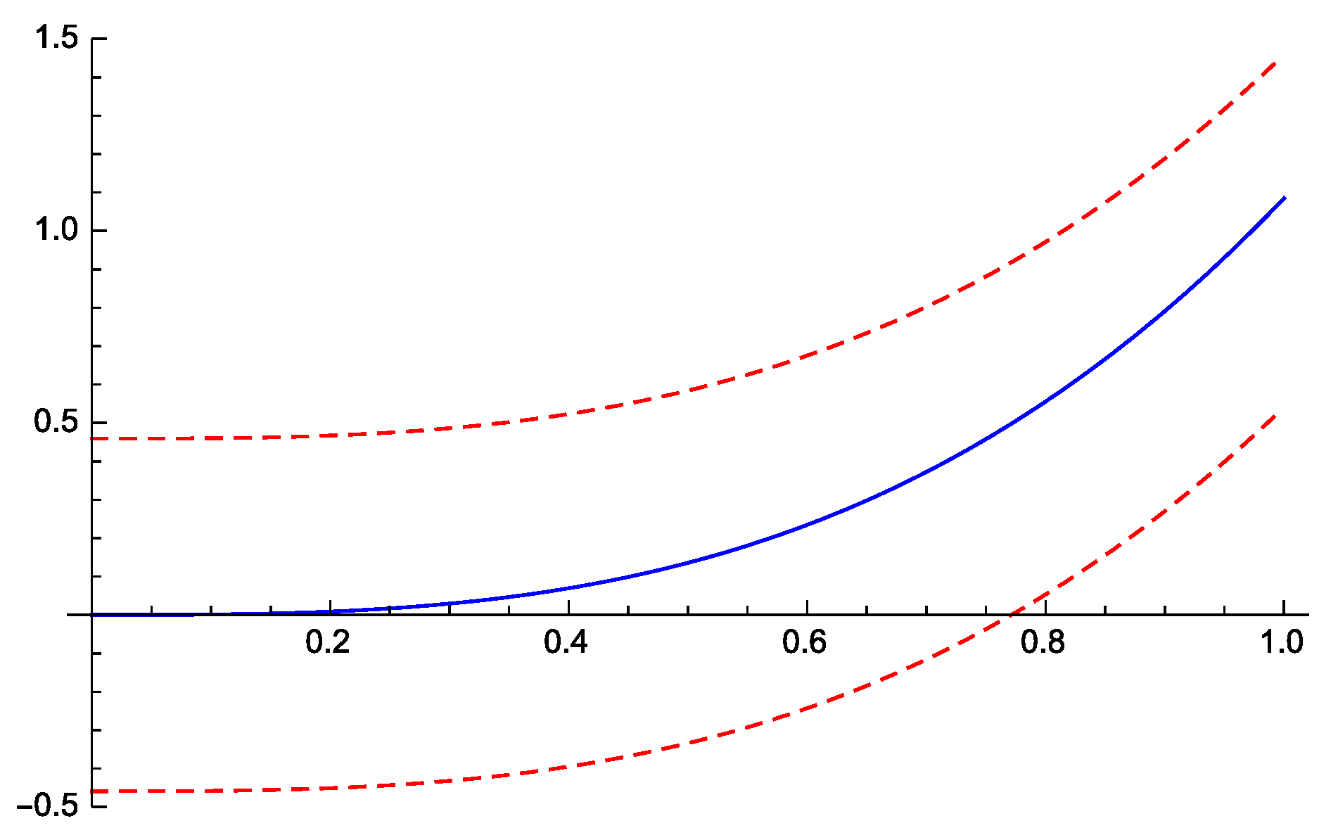
Choose $m=8$, $\lambda =7/5$, $\tilde{\mathit{x}}=\mathit{v}$ and hence $K=0.2471\dots$, $\beta =1.2179\dots$, $\eta =0.0665\dots$ and $K\beta \eta =0.0200\dots$ As $K\beta \eta <0.1547\dots$, it follows, from Theorem 1, that the best ball of location of solution is $\overline{B(\mathit{v},0.0686\dots )}$ and the biggest ball of convergence is $B(\mathit{v},1.5259\dots )$.

If the starting point for Newton’s method is $x_0=\mathit{v}$, the method converges to the solution $x^{*}={(x_1^{*},x_2^{*},\dots ,x_8^{*})}^t$ of system (14), which is shown in

Table 2. Numerical solution $x^{*}$ of system (14) with $\lambda =7/5$.

i	${\mathit{x}}_{\mathit{i}}^{*}$	i	${\mathit{x}}_{\mathit{i}}^{*}$
1	0.02267000…	5	0.65888692…
2	0.11607746…	6	0.82291926…
3	0.27057507…	7	0.93276524…
4	0.46275932…	8	0.98797444…

, after four iterations with stopping criterion $\parallel x_n-x_{n-1}{\parallel }_{\infty }<{10}^{-18}$, $n\in \mathbb{N}$.

Moreover, errors $\parallel x^{*}-x_n\parallel$ and sequence $\{\parallel F\left(x_n\right)\parallel \}$ are shown in

Table 3. Absolute errors and $\{\parallel F\left(x_n\right)\parallel \}$.

n	$\parallel {\mathit{x}}^{*}-{\mathit{x}}_{\mathit{n}}\parallel$	$\parallel \mathit{F}\left({\mathit{x}}_{\mathit{n}}\right)\parallel$
0	$6.7169\dots \times {10}^{-2}$	$9.6624\dots \times {10}^{-1}$
1	$6.4734\dots \times {10}^{-4}$	$5.3956\dots \times {10}^{-4}$
2	$6.0570\dots \times {10}^{-8}$	$5.0516\dots \times {10}^{-8}$
3	$5.4063\dots \times {10}^{-16}$	$4.5077\dots \times {10}^{-16}$

. Observe then that vector shown in Table 2 is a good approximation of a solution of (14).

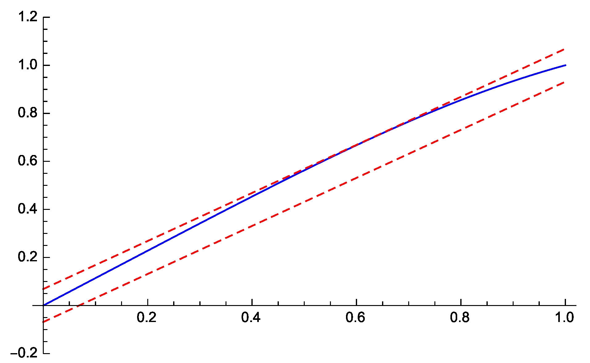
Furthermore, as a solution of (12) satisfies $x\left(0\right)=0$ and $x\left(1\right)=1$, if values of Table 2 are interpolated, an approximated solution is obtained, which is painted in Figure 2. Notice that this approximated solution lies in the domain of location of solution $\overline{B(\mathit{v},0.0686\dots )}$ which is obtained from Theorem 1.

6. Conclusions

Following the idea of the Fixed Point Theorem for the method of successive approximations, we do an analysis for Newton’s method, use the theoretical significance of the method to prove the existence and uniqueness of solution of a particular type of nonlinear integral equations of Fredholm and, in addition, obtain a domain of global convergence for the method that allows locating a solution and separating it from other possible solutions. For this, we use a technique based on using auxiliary points. Moreover, we present a study of the nonlinear equations which is based on the real parameter involved in the equation.