Numerical Solution of the Boundary Value Problems Arising in Magnetic Fields and Cylindrical Shells


 ,
,  ,
,  and
and
Abstract
1. Introduction
2. Fundamentals of Cubic B-Splines
3. Cubic-B Spline Solutions of 8th Order BVP
4. Application of Cubic B Spline on Linear 8th Order BVP’s
5. Application of Cubic B Spline on Non-Linear 8th Order BVP’s
6. Convergence Analysis
7. Results and Discussion
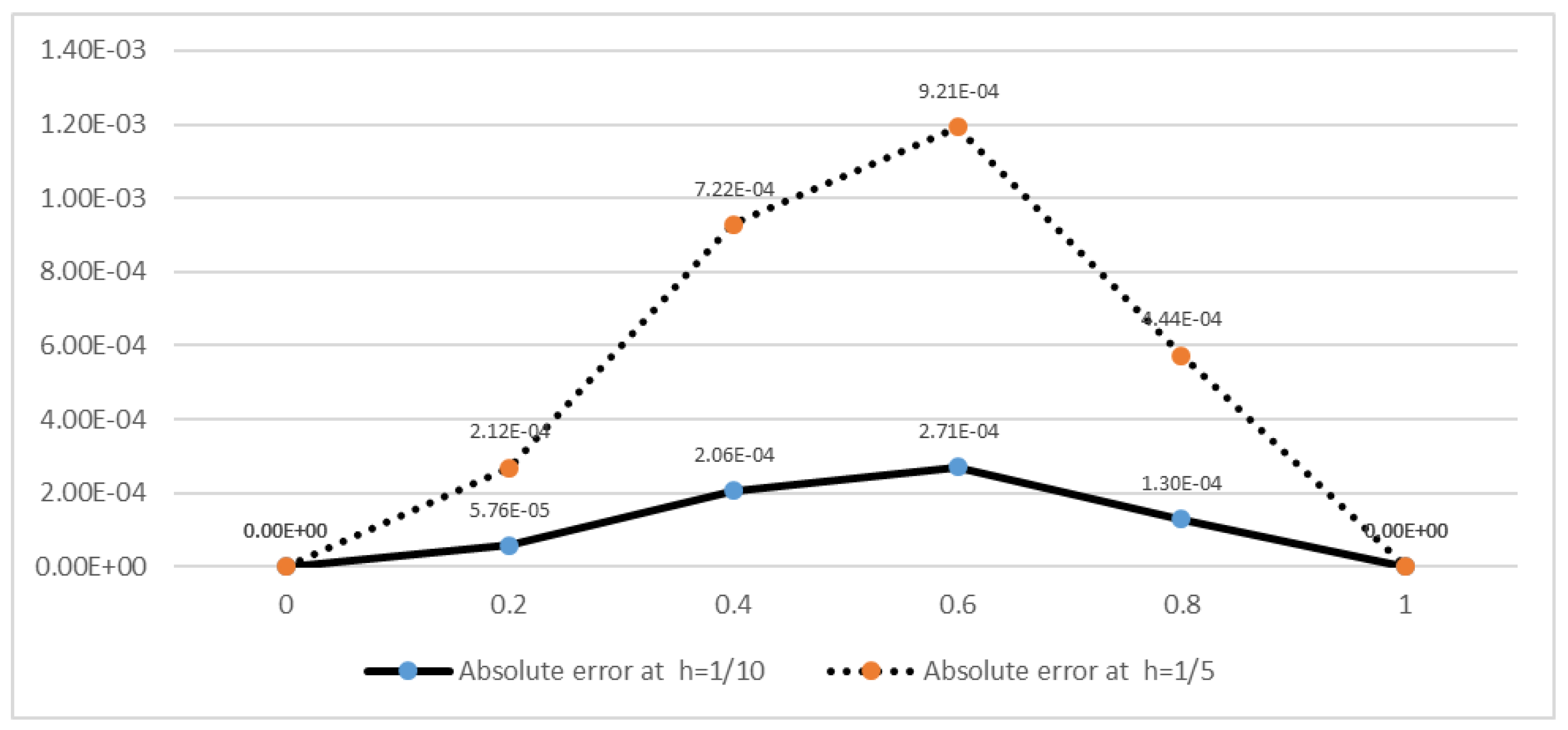
7.1. Problem 1
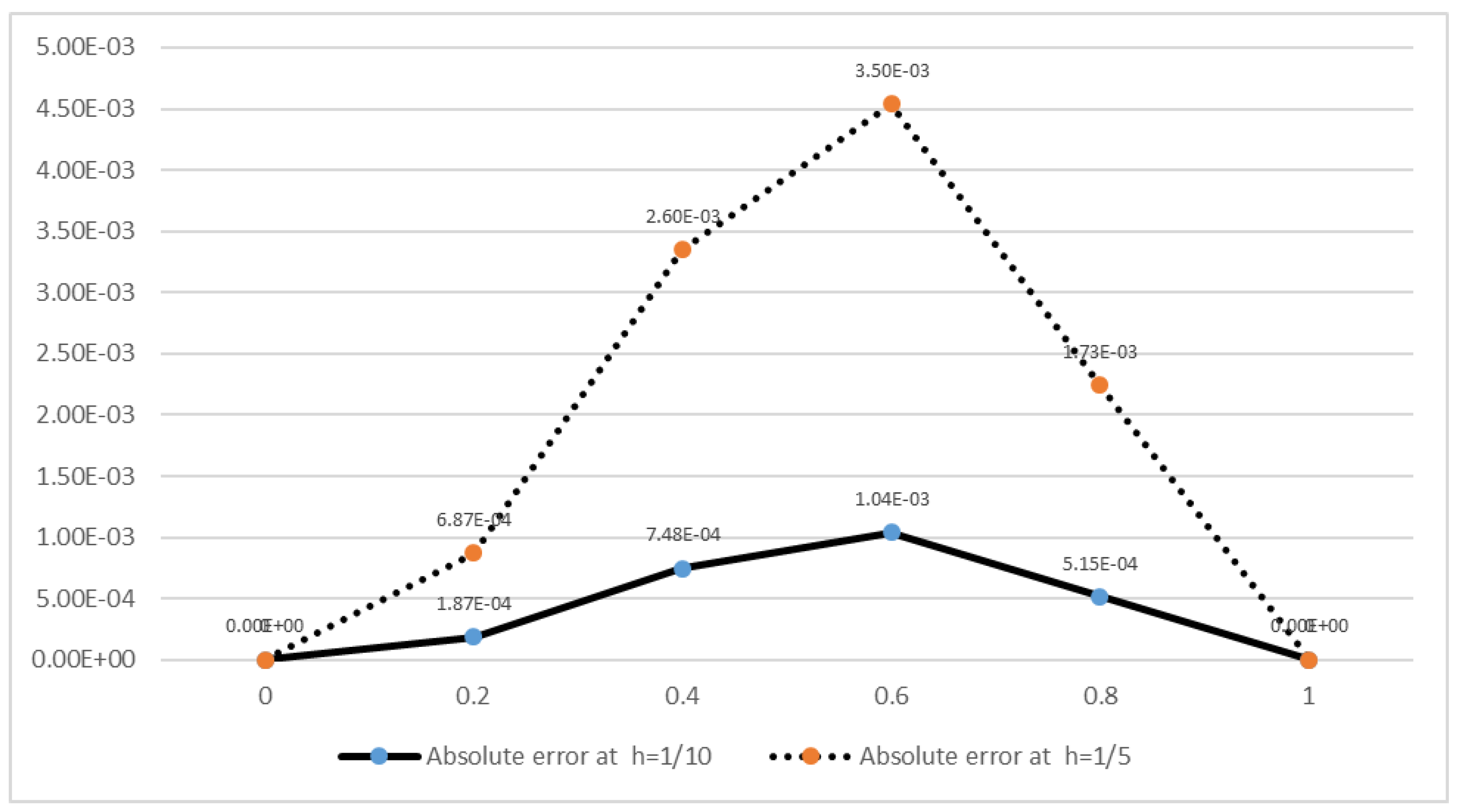
7.2. Problem 2
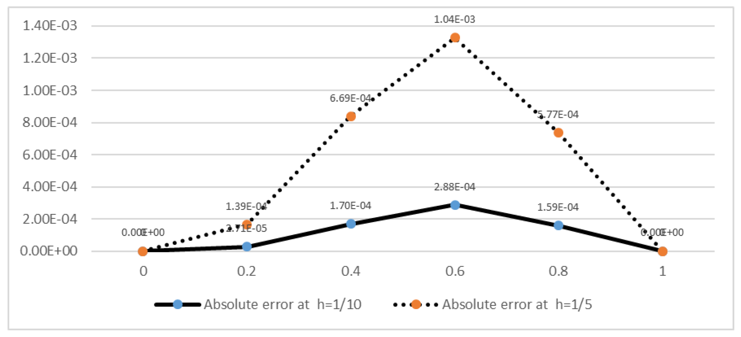
7.3. Problem 3
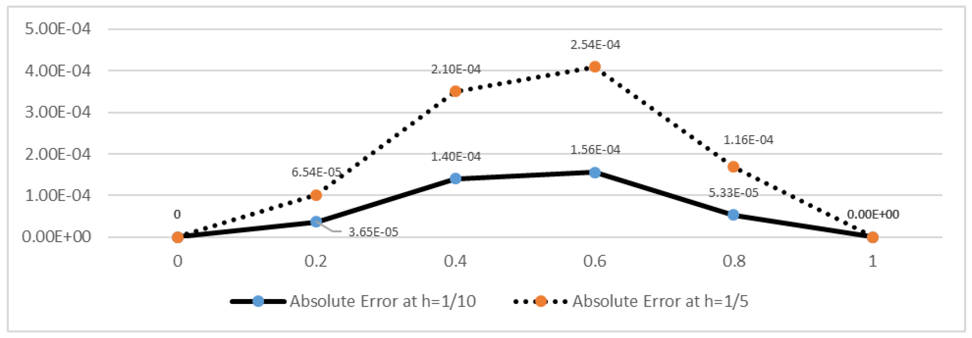
7.4. Problem 4
7.5. Problem 5
7.6. Problem 6
8. Conclusions
Author Contributions
Funding
Conflicts of Interest
Abbreviations
| ADM | Adomian decomposition method |
| BVP’s | Boundary value problems |
References
- Agarwal, R.P. Boundary Value Problems from Higher Order Differential Equations; World Scientific: Singapore, 1986. [Google Scholar]
- Akram, G.; Rehman, H.U. Numerical solution of 8th order boundary value problems in reproducing Kernel space. Numer. Algorithms 2013, 62, 527–540. [Google Scholar] [CrossRef]
- Akram, G.; Siddiqi, S.S. Nonic spline solutions of 8th order boundary value problems. Appl. Math. Comput. 2006, 182, 829–845. [Google Scholar]
- Bishop, R.; Cannon, S.; Miao, S. On coupled bending and torsional vibration of uniform beams. J. Sound Vib. 1989, 131, 457–464. [Google Scholar] [CrossRef]
- Boutayeb, A.; Twizell, E. Finite-difference methods for the solution of special 8th-order boundary-value problems. Int. J. Comput. Math. 1993, 48, 63–75. [Google Scholar] [CrossRef]
- Caglar, H.; Caglar, N.; Elfaituri, K. B-spline interpolation compared with finite difference, finite element and finite volume methods which applied to two-point boundary value problems. Appl. Math. Comput. 2006, 175, 72–79. [Google Scholar] [CrossRef]
- Chandrasekhar, S. Hydrodynamic and Hydromagnetic Stability; Courier Corporation: New York, NY, USA, 2013. [Google Scholar]
- De Boor, C. On the convergence of odd-degree spline interpolation. J. Approx. Theory 1968, 1, 452–463. [Google Scholar] [CrossRef]
- Dehghan, M.; Lakestani, M. Numerical solution of nonlinear system of second-order boundary value problems using cubic B-spline scaling functions. Int. J. Comput. Math. 2008, 85, 1455–1461. [Google Scholar] [CrossRef]
- Davies, A.; Karageorghis, A.; Phillips, T. Spectral Galerkin methods for the primary 2-point boundary value problem in modelling viscoelastic flows. Int. J. Numer. Methods Eng. 1988, 26, 647–662. [Google Scholar] [CrossRef]
- Djidjeli, K.; Twizell, E.; Boutayeb, A. Numerical methods for special nonlinear boundary-value problems of order 2m. J. Comput. Appl. Math. 1993, 47, 35–45. [Google Scholar]
- Elahi, Z.; Akram, G.; Siddiqi, S.S. Numerical solution for solving special 8th-order linear boundary value problems using Legendre Galerkin method. Math. Sci. 2016, 10, 201–209. [Google Scholar] [CrossRef]
- Gupta, Y.; Kumar, M. B-spline method for solution of linear fourth order boundary value problem. System 2011, 1, 4. [Google Scholar]
- Prenter, P.M. Splines and Variational Methods; Courier Corporation: New York, NY, USA, 2008. [Google Scholar]
- Hall, C. On error bounds for spline interpolation. J. Approx. Theory 1968, 1, 209–218. [Google Scholar] [CrossRef]
- Golbabai, A.; Javidi, M. Application of homotopy perturbation method for solving 8th-order boundary value problems. Appl. Math. Comput. 2007, 191, 334–346. [Google Scholar]
- Haq, S.; Idrees, M.; Islam, S. Application of optimal Homotopy asymptotic method to 8th order initial and boundary value problems. Int. J. Appl. Math. Comput. 2010, 2, 73–80. [Google Scholar]
- He, J.-H. A coupling method of a homotopy technique and a perturbation technique for non-linear problems. Int. J. Non-Linear Mech. 2000, 35, 37–43. [Google Scholar] [CrossRef]
- Inç, M.; Evans, D.J. An efficient approach to approximate solutions of 8th-order boundary-value problems. Int. J. Comput. Math. 2004, 81, 685–692. [Google Scholar] [CrossRef]
- Khalid, A.; Naeem, M.N. Cubic B-spline Solution of Nonlinear Sixth Order Boundary Value Problems. J. Math. 2018, 50, 91–103. [Google Scholar]
- Lang, F.-G.; Xu, X.-P. A new cubic B-spline method for linear fifth order boundary value problems. J. Appl. Math. Comput. 2011, 36, 101–116. [Google Scholar] [CrossRef]
- Li, C.-L.; Cui, M.-G. The exact solution for solving a class nonlinear operator equations in the reproducing kernel space. Appl. Math. Comput. 2003, 143, 393–399. [Google Scholar] [CrossRef]
- Liu, G.; Wu, T. Differential quadrature solutions of 8th-order boundary-value differential equations. J. Comput. Appl. Math. 2002, 145, 223–235. [Google Scholar] [CrossRef]
- Meštrović, M. The modified decomposition method for 8th-order boundary value problems. Appl. Math. Comput. 2007, 188, 1437–1444. [Google Scholar]
- Mohyud-Din, S.T.; Noor, M.A.; Noor, K.I. Exp-function method for solving higher-order boundary value problems. Bull. Inst. Math. Acad. Sin. New Ser. 2009, 4, 219–234. [Google Scholar]
- Noor, M.A.; Mohyud-Din, S. Homotopy method for solving 8th order boundary value problems. J. Math. Anal. Approx. Theory 2006, 1, 161–169. [Google Scholar]
- Noor, M.A.; Mohyud-Din, S.T. Homotopy perturbation method for solving nonlinear higher-order boundary value problems. Int. J. Nonlinear Sci. Numer. Simul. 2008, 9, 395–408. [Google Scholar] [CrossRef]
- Noor, M.A.; Mohyud-Din, S.T. Variational iteration method for solving higher-order nonlinear boundary value problems using He’s polynomials. Int. J. Nonlinear Sci. Numer. Simul. 2008, 9, 141–156. [Google Scholar] [CrossRef]
- Paliwal, D.; Pande, A. Orthotropic cylindrical pressure vessels under line load. Int. J. Press. Vessels Pip. 1999, 76, 455–459. [Google Scholar] [CrossRef]
- Reddy, A.P.; Harageri, M.; Sateesha, C. A numerical approach to solve 8th order boundary value problems by Haar wavelet collocation method. J. Math. Model. 2017, 5, 61–75. [Google Scholar]
- Reddy, S.M. Numerical solution of 8th order boundary value problems by Petrov-Galerkin method with quintic B-splines as basic functions and septic B-splines as weight functions. Int. J. Eng. Comput. Sci. 2016, 5, 17894–17901. [Google Scholar]
- Sharma, S.K. Free Vibrations of Circular Cylindrical Shells. Master’s Thesis, Missouri University of Science and Technology, Rolla, MO, USA, 1971. [Google Scholar]
- Shen, I. Hybrid damping through intelligent constrained layer treatments. J. Vib. Acoust. 1994, 116, 341–349. [Google Scholar] [CrossRef]
- Viswanadham, K.K.; Raju, Y.S. Quintic B-Spline Collocation Method for 8th boundary value problems. Adv. Comput. Math. Appl. 2012, 1, 47–52. [Google Scholar]
- Viswanadham, K.K.; Raju, Y.S. Sextic B-Spline Collocation Method for 8th Order Boundary Value Problems. Int. J. Appl. Sci. Eng. 2014, 12, 43–57. [Google Scholar]
- Viswanadham, K.K.; Ballem, S. Numerical Solution of 8th Order Boundary Value Problems by Galerkin Method with Quintic B-splines. Int. J. Comput. Appl. 2014, 89, 7–13. [Google Scholar]
- Viswanadham, K.K.; Raju, Y.S. Numerical solution of 8th order boundary value problems by Galerkin method with septic B-splines. Procedia Eng. 2015, 127, 1370–1377. [Google Scholar] [CrossRef]
- Wazwaz, A.-M. The numerical solution of special 8th-order boundary value problems by the modified decomposition method. Neural Parallel Sci. Comput. 2000, 8, 133–146. [Google Scholar]


| 0 | 0 | 0 | |
| 1/6 | |||
| 4/6 | 0 | −2/ | |
| 1/6 | −1/2h | 1/ | |
| , and all others | 0 | 0 | 0 |
| z | Exact Solution of | Cubic B-Spline Solution | Absolute Error of CBS | [31] |
|---|---|---|---|---|
| 0 | 1 | 1 | 0 | 0 |
| 0.1 | 0.99465382626808 | 0.99464003039971 | 1.38 | 5.96 |
| 0.2 | 0.97712220652814 | 0.97706460667836 | 5.76 | 6.56 |
| 0.3 | 0.94490116530320 | 0.94477345208706 | 1.28 | 1.19 |
| 0.4 | 0.89509481858476 | 0.89488924463764 | 2.06 | 9.54 |
| 0.5 | 0.82436063535006 | 0.82409833674802 | 2.62 | 2.03 |
| 0.6 | 0.72884752015620 | 0.72857639555592 | 2.71 | 3.70 |
| 0.7 | 0.60412581224114 | 0.60390411609609 | 2.22 | 5.07 |
| 0.8 | 0.44510818569849 | 0.44497804890510 | 1.30 | 4.29 |
| 0.9 | 0.24596031111570 | 0.24592145969977 | 3.89 | 2.15 |
| 1 | 0 | 0 | 0 | 0 |
| z | Exact Solution of | Cubic B-Spline Solution | Absolute Error of CBS |
|---|---|---|---|
| 0 | 1 | 1 | 0 |
| 0.2 | 0.97712220652814 | 0.97691002752530 | 2.12 |
| 0.4 | 0.89509481858476 | 0.89437324656962 | 7.22 |
| 0.6 | 0.72884752015620 | 0.72792627066555 | 9.21 |
| 0.8 | 0.44510818569849 | 0.44466410737581 | 4.44 |
| 1 | 0 | 0 | 0 |
| z | Cubic B-Spline Solution of | Exact Solution of | Absolute Error of | Exact Solution of | Cubic B-Spline Solution of | Absolute Error of | Exact Solution of | Cubic B-Spline Solution of | Absolute Error of |
|---|---|---|---|---|---|---|---|---|---|
| 0 | 0 | 0 | 0 | −1 | −1 | 0 | −2 | −2 | 0 |
| 0.1 | −0.1105 | −0.1108 | 2.82 | −1.2157 | −1.2160 | 2.94 | −2.3208 | −2.3267 | 5.87 |
| 0.2 | −0.2443 | −0.2449 | 5.85 | −1.4649 | −1.4653 | 3.38 | −2.6738 | −2.6805 | 6.62 |
| 0.3 | −0.4049 | −0.4057 | 7.79 | −1.7493 | −1.7521 | 2.74 | −3.0637 | −3.0842 | 2.05 |
| 0.4 | −0.5966 | −0.5974 | 7.20 | −2.0758 | −2.0822 | 6.37 | −3.5308 | −3.5556 | 2.48 |
| 0.5 | −0.8243 | −0.8247 | 3.58 | −2.4533 | −2.4632 | 9.88 | −4.0926 | −4.1072 | 1.46 |
| 0.6 | −1.0928 | −1.0931 | 2.11 | −2.8918 | −2.9036 | 1.18 | −4.7375 | −4.7464 | 8.87 |
| 0.7 | −1.4081 | −1.4089 | 7.61 | −3.4016 | −3.4125 | 1.09 | −5.4371 | −5.4755 | 3.84 |
| 0.8 | −1.7783 | −1.7794 | 1.01 | −3.9914 | −3.9987 | 7.24 | −6.2315 | −6.2921 | 6.06 |
| 0.9 | −2.2121 | −2.2129 | 7.34 | −4.6685 | −4.6709 | 2.34 | −7.1329 | −7.1892 | 5.63 |
| 1 | −2.7183 | −2.7183 | 0 | −5.4365 | −5.4365 | 0 | −8.1548 | −8.1548 | 0 |
| z | Exact Solution of | Cubic B-Spline Solution | Absolute Error of CBS | [31] |
|---|---|---|---|---|
| 0 | 0 | 0 | 0 | 0 |
| 0.1 | 0.09946538262681 | 0.09942405954487 | 4.13 | 2.46 |
| 0.2 | 0.19542444130563 | 0.19523703705762 | 1.87 | 8.19 |
| 0.3 | 0.28347034959096 | 0.28302687772238 | 4.43 | 1.99 |
| 0.4 | 0.35803792743391 | 0.35728987754939 | 7.48 | 4.29 |
| 0.5 | 0.41218031767503 | 0.41119364975850 | 9.87 | 6.19 |
| 0.6 | 0.43730851209372 | 0.43626438816196 | 1.04 | 7.18 |
| 0.7 | 0.42288806856880 | 0.42202025044259 | 8.68 | 7.03 |
| 0.8 | 0.35608654855880 | 0.35557187302869 | 5.15 | 5.06 |
| 0.9 | 0.22136428000413 | 0.22121010545131 | 1.54 | 2.41 |
| 1 | 0 | 0 | 0 | 0 |
| z | Exact Solution of | Cubic B-Spline Solution | Absolute Error of CBS |
|---|---|---|---|
| 0 | 0 | 0 | 0 |
| 0.2 | 0.19542444130563 | 0.19473719409835 | 6.87 |
| 0.4 | 0.35803792743391 | 0.35543924551290 | 2.60 |
| 0.6 | 0.43730851209372 | 0.43381262638307 | 3.50 |
| 0.8 | 0.35608654855880 | 0.35435927825085 | 1.73 |
| 1 | 0 | 0 | 0 |
| z | Cubic B-Spline Solution of | Exact Solution of | Absolute Error of | Exact Solution of | Cubic B-Spline Solution of | Absolute Error of | Exact Solution of | Cubic B-Spline Solution of | Absolute Error of |
|---|---|---|---|---|---|---|---|---|---|
| 0 | 1 | 1 | 0 | 0 | 0 | 0 | −3 | −3 | 0 |
| 0.1 | 0.9836 | 0.9827 | 8.80 | −0.3426 | −0.3456 | 2.96 | −3.8792 | −3.922 | 4.28 |
| 0.2 | 0.9282 | 0.9262 | 2.04 | −0.7817 | −0.7844 | 2.69 | −4.9174 | −4.9259 | 8.54 |
| 0.3 | 0.8235 | 0.8205 | 2.95 | −1.3251 | −1.3307 | 5.61 | −6.0474 | −6.1216 | 7.42 |
| 0.4 | 0.6564 | 0.6535 | 2.91 | −1.9885 | −2.0087 | 2.02 | −7.4939 | −7.5959 | 1.02 |
| 0.5 | 0.4122 | 0.4106 | 1.62 | −2.8146 | −2.8499 | 3.53 | −9.3467 | −9.4134 | 6.67 |
| 0.6 | 0.0741 | 0.0735 | 6.11 | −3.8470 | −3.8914 | 4.44 | −11.5887 | −11.6174 | 2.87 |
| 0.7 | −0.3768 | −0.3797 | 2.87 | −5.1312 | −5.1734 | 4.22 | −14.0766 | −14.2306 | 1.54 |
| 0.8 | −0.9714 | −0.9753 | 3.95 | −6.7094 | −6.7375 | 2.81 | −17.0029 | −17.2559 | 2.53 |
| 0.9 | −1.7405 | −1.7434 | 2.92 | −8.6160 | −8.6246 | 8.62 | −20.4391 | −20.6781 | 2.39 |
| 1 | −2.7183 | −2.7183 | 0 | −10.8731 | −10.8731 | 0 | −24.4645 | −24.4645 | 0 |
| z | Exact Solution of | Cubic B-Spline Solution | Absolute Error of CBS | [23] |
|---|---|---|---|---|
| 0 | 0 | 0 | 0 | 0 |
| 0.1 | −0.09883508248036 | −0.09883929795528 | 4.22 | 3.97 |
| 0.2 | −0.19072255756326 | −0.19074966511972 | 2.71 | 9.32 |
| 0.3 | −0.26892338806182 | −0.26900781261417 | 8.44 | 6.78 |
| 0.4 | −0.32711140753927 | −0.32728094968339 | 1.70 | 1.08 |
| 0.5 | −0.35956915395315 | −0.35982014743648 | 2.51 | 1.83 |
| 0.6 | −0.36137118297282 | −0.36165941441105 | 2.88 | 3.21 |
| 0.7 | −0.32855102049122 | −0.32880597250785 | 2.55 | 6.73 |
| 0.8 | −0.25824819272383 | −0.25840750142588 | 1.59 | 1.27 |
| 0.9 | −0.14883211282922 | −0.14888246114063 | 5.03 | 2.47 |
| 1 | 0 | 0 | 0 | 0 |
| z | Exact Solution of | Cubic B-Spline Solution | Absolute Error of CBS |
|---|---|---|---|
| 0 | 0 | 0 | 0 |
| 0.2 | −0.19072255756326 | −0.19086203871595 | 1.39 |
| 0.4 | −0.32711140753927 | −0.32778034786133 | 6.69 |
| 0.6 | −0.36137118297282 | −0.36241298481970 | 1.04 |
| 0.8 | −0.25824819272383 | −0.25882550188894 | 5.77 |
| 1 | 0 | 0 | 0 |
| z | Cubic B-Spline Solution of | Exact Solution of | Absolute Error of | Exact Solution of | Cubic B-Spline Solution of | Absolute Error of | Exact Solution of | Cubic B-Spline Solution of | Absolute Error of |
|---|---|---|---|---|---|---|---|---|---|
| 0 | −1 | −1 | 0 | 0 | 0 | 0 | 7 | 7 | 0 |
| 0.1 | −0.9651 | −0.9652 | 9.15 | 0.6965 | 0.6964 | 8.24 | 6.8952 | 6.8584 | 3.68 |
| 0.2 | −0.8614 | −0.8618 | 3.78 | 1.3721 | 1.3717 | 4.41 | 6.5829 | 6.559 | 2.39 |
| 0.3 | −0.6921 | −0.6928 | 7.36 | 2.0101 | 2.0082 | 1.85 | 6.0785 | 6.074 | 4.53 |
| 0.4 | −0.4621 | −0.463 | 8.89 | 2.5933 | 2.5865 | 6.82 | 5.4152 | 5.3903 | 2.49 |
| 0.5 | −0.1788 | −0.1794 | 6.47 | 3.0990 | 3.0863 | 1.27 | 4.5338 | 4.5096 | 2.42 |
| 0.6 | 0.1493 | 0.1493 | 3.15 | 3.5053 | 3.4884 | 1.69 | 3.4479 | 3.4477 | 2.11 |
| 0.7 | 0.5132 | 0.5125 | 7.00 | 3.7931 | 3.7758 | 1.73 | 2.2734 | 2.2348 | 3.86 |
| 0.8 | 0.8992 | 0.8981 | 1.14 | 3.9482 | 3.9353 | 1.29 | 0.9878 | 0.9146 | 7.32 |
| 0.9 | 1.2937 | 1.2928 | 9.15 | 3.9642 | 3.9587 | 5.46 | −0.3822 | −0.456 | 7.38 |
| 1 | 1.6829 | 1.6829 | 0 | 3.8442 | 3.8442 | 0 | −1.8070 | −1.8070 | 0 |
| z | Exact Solution | Presented Method Solution | Absolute Error | [30] |
|---|---|---|---|---|
| 0 | 1 | 1 | 0 | 0 |
| 0.1 | 1.10517091807564 | 1.10517794712470 | 7.03 | 2.50 |
| 0.2 | 1.22140275816017 | 1.22143922353981 | 3.65 | 8.94 |
| 0.3 | 1.34985880757600 | 1.34994628964200 | 8.75 | 1.56 |
| 0.4 | 1.49182469764127 | 1.49196477025922 | 1.40 | 1.82 |
| 0.5 | 1.64872127070012 | 1.64888916217970 | 1.68 | 8.82 |
| 0.6 | 1.82211880039050 | 1.82227459457679 | 1.56 | 7.51 |
| 0.7 | 2.01375270747047 | 2.01386242544904 | 1.10 | 1.88 |
| 0.8 | 2.22554092849246 | 2.22559418213629 | 5.33 | 1.93 |
| 0.9 | 2.45960311115695 | 2.45961577150042 | 1.27 | 1.16 |
| 1 | 2.71828182845905 | 2.71828182845905 | 0 | 0 |
| z | Exact Solution | Presented Method Solution | Absolute Error |
|---|---|---|---|
| 0 | 1 | 1 | 0 |
| 0.2 | 1.22140275816017 | 1.22146817204786 | 6.54 |
| 0.4 | 1.49182469764127 | 1.49203484074618 | 2.10 |
| 0.6 | 1.82211880039050 | 1.82237276345783 | 2.54 |
| 0.8 | 2.22554092849246 | 2.22565718003072 | 1.16 |
| 1 | 2.71828182845905 | 2.71828182845905 | 0 |
| z | Cubic B-Spline Solution of | Exact Solution of | Absolute Error of | Exact Solution of | Cubic B-Spline Solution of | Absolute Error of | Exact Solution of | Cubic B-Spline Solution of | Absolute Error of |
|---|---|---|---|---|---|---|---|---|---|
| 0 | 1 | 1 | 0 | 1 | 1 | 0 | 1 | 1 | 0 |
| 0.1 | 1.1055 | 1.10534 | 1.67 | 1.1084 | 1.10677 | 1.60 | 1.1241 | 1.11462 | 9.45 |
| 0.2 | 1.2222 | 1.22182 | 4.20 | 1.2244 | 1.22292 | 1.52 | 1.2214 | 1.2112 | 1.02 |
| 0.3 | 1.3510 | 1.35042 | 5.61 | 1.3499 | 1.34901 | 8.51 | 1.3499 | 1.32485 | 2.50 |
| 0.4 | 1.4927 | 1.49226 | 4.40 | 1.4918 | 1.48789 | 3.93 | 1.4918 | 1.46978 | 2.20 |
| 0.5 | 1.6489 | 1.64881 | 8.64 | 1.6487 | 1.64296 | 5.76 | 1.6487 | 1.6449 | 3.82 |
| 0.6 | 1.8221 | 1.8218 | 3.19 | 1.8221 | 1.81687 | 5.25 | 1.8581 | 1.84009 | 1.80 |
| 0.7 | 2.0138 | 2.01319 | 5.60 | 2.0138 | 2.01098 | 2.77 | 2.0730 | 2.04339 | 2.96 |
| 0.8 | 2.2255 | 2.22502 | 5.22 | 2.2256 | 2.22555 | 1.03 | 2.2718 | 2.24865 | 2.31 |
| 0.9 | 2.4596 | 2.45933 | 2.71 | 2.4618 | 2.46071 | 1.11 | 2.4677 | 2.46365 | 4.05 |
| 1 | 2.7182 | 2.7182 | 0 | 2.7182 | 2.7182 | 0 | 2.7182 | 2.7182 | 0 |
| z | Exact Solution | Presented Method Solution | Absolute Error | [30] | [34] | [36] | [37] |
|---|---|---|---|---|---|---|---|
| 0 | 0 | 0 | 0 | 0 | 0 | 0 | 0 |
| 0.064 | 0.0628547262 | 0.0628509884 | 3.74 | 3.42 | 1.42 | 2.01 | 2.94 |
| 0.129 | 0.1219912885 | 0.1219786318 | 1.27 | 4.10 | 1.07 | 4.54 | 1.58 |
| 0.194 | 0.1778251212 | 0.1778037262 | 2.14 | 2.68 | 3.37 | 1.52 | 2.91 |
| 0.259 | 0.2307057020 | 0.2306800632 | 2.56 | 1.42 | 7.02 | 4.07 | 4.91 |
| 0.324 | 0.2809298146 | 0.2809058296 | 2.40 | 3.34 | 9.54 | 6.71 | 7.34 |
| 0.389 | 0.3287516379 | 0.3287337725 | 1.79 | 5.84 | 1.07 | 9.06 | 8.51 |
| 0.454 | 0.3743905291 | 0.3743802408 | 1.03 | 7.90 | 1.03 | 1.00 | 6.54 |
| 0.518 | 0.4180371082 | 0.4180329583 | 4.15 | 4.80 | 5.22 | 5.45 | 4.38 |
| 0.583 | 0.4598580678 | 0.4598572086 | 8.59 | 2.41 | 2.41 | 2.59 | 2.31 |
| 0.648 | 0.5 | 0.5 | 0 | 0 | 0 | 0 | 0 |
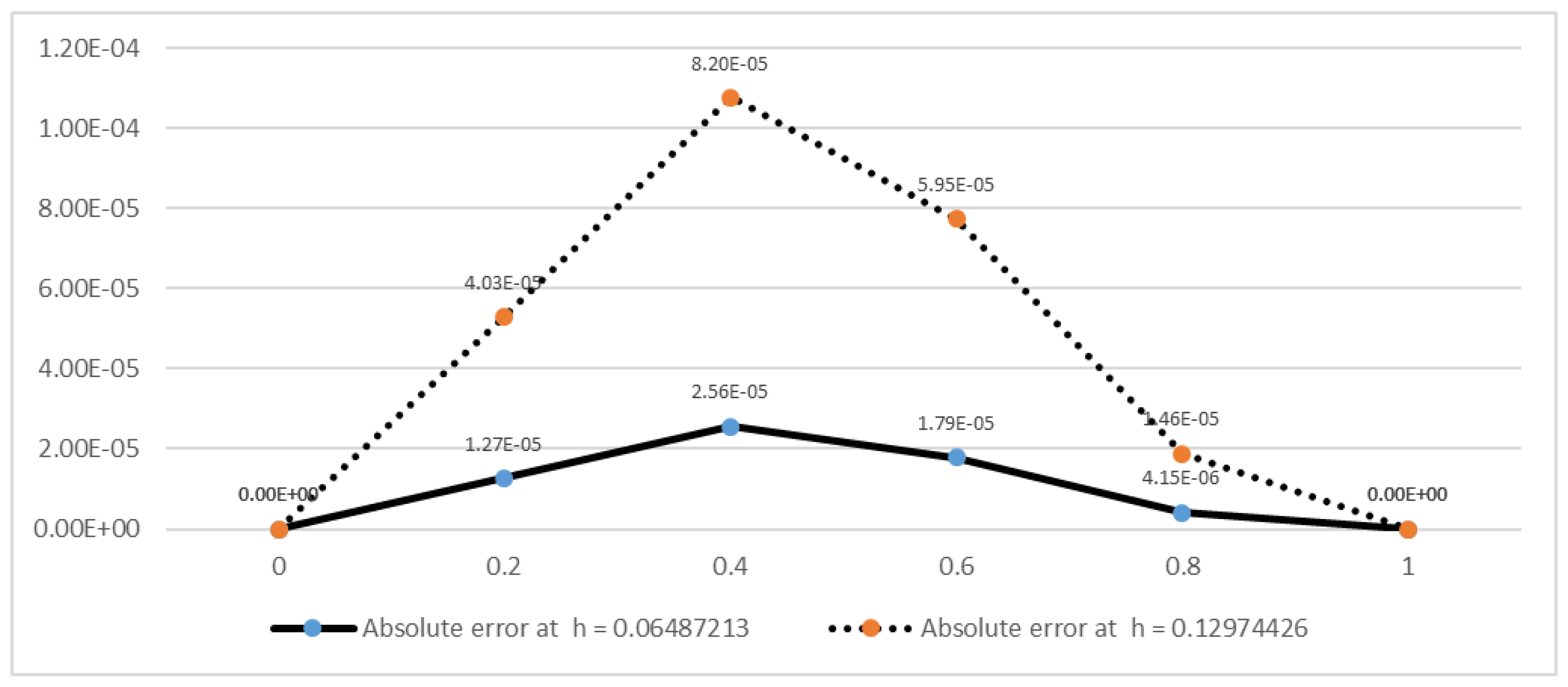
| z | Exact Solution | Presented Method Solution | Absolute Error |
|---|---|---|---|
| 0 | 0 | 0 | 0 |
| 0.129 | 0.12199128852626 | 0.12195103139582 | 4.03 |
| 0.259 | 0.23070570204092 | 0.23062366023811 | 8.20 |
| 0.389 | 0.32875163792382 | 0.32869211718688 | 5.95 |
| 0.518 | 0.41803710829203 | 0.41802254868918 | 1.46 |
| 0.648 | 0.5 | 0.5 | 0 |
| z | Cubic B-Spline Solution of | Exact Solution of | Absolute Error of | Exact Solution of | Cubic B-Spline Solution of | Absolute Error of | Exact Solution of | Cubic B-Spline Solution of | Absolute Error of |
|---|---|---|---|---|---|---|---|---|---|
| 0 | 0 | 0 | 0 | 0 | 0 | 0 | 0 | 0 | 0 |
| 0.064 | 0.9399 | 0.93897 | 8.81 | −0.8799 | −0.8816 | 1.73 | 1.6984 | 1.67938 | 1.90 |
| 0.129 | 0.8857 | 0.885 | 7.35 | −0.7797 | −0.7821 | 2.42 | 1.4326 | 1.41121 | 2.14 |
| 0.194 | 0.8375 | 0.83698 | 5.41 | −0.6955 | −0.6985 | 2.95 | 1.2001 | 1.18751 | 1.26 |
| 0.259 | 0.7943 | 0.79395 | 3.28 | −0.6252 | −0.628 | 2.85 | 1.0041 | 1.00314 | 9.46 |
| 0.324 | 0.7553 | 0.75515 | 1.40 | −0.5662 | −0.5683 | 2.12 | 0.8617 | 0.85397 | 7.75 |
| 0.389 | 0.7199 | 0.71994 | 7.23 | −0.5162 | −0.5172 | 1.08 | 0.7463 | 0.73574 | 1.06 |
| 0.454 | 0.6879 | 0.68782 | 6.17 | −0.4727 | −0.4729 | 1.31 | 0.6506 | 0.64331 | 7.33 |
| 0.518 | 0.6588 | 0.65841 | 3.50 | −0.4336 | −0.4338 | 1.93 | 0.5718 | 0.57012 | 1.64 |
| 0.583 | 0.6317 | 0.6314 | 3.10 | −0.3988 | −0.3989 | 1.50 | 0.5116 | 0.50788 | 3.70 |
| 0.648 | 0.6065 | 0.6065 | 0 | −0.3678 | −0.3678 | 0 | 0.4462 | 0.4462 | 0 |
| z | Exact Solution | Presented Method Solution | Absolute Error | [30] | [36] |
|---|---|---|---|---|---|
| 0 | 1 | 1 | 0 | 0 | 0 |
| 0.1 | 0.90483741803596 | 0.90484101917459 | 3.60 | 6.56 | 3.58 |
| 0.2 | 0.81873075307798 | 0.81874287120508 | 1.21 | 9.54 | 6.32 |
| 0.3 | 0.74081822068172 | 0.74083908532179 | 2.09 | 4.11 | 1.90 |
| 0.4 | 0.67032004603564 | 0.67034596914992 | 2.59 | 6.74 | 3.10 |
| 0.5 | 0.60653065971263 | 0.60655628570162 | 2.56 | 8.76 | 3.64 |
| 0.6 | 0.54881163609403 | 0.54883230312747 | 2.07 | 8.40 | 3.17 |
| 0.7 | 0.49658530379141 | 0.49659863075283 | 1.33 | 5.84 | 1.93 |
| 0.8 | 0.44932896411722 | 0.44933526163887 | 6.30 | 2.95 | 7.18 |
| 0.9 | 0.40656965974060 | 0.40657124798308 | 1.59 | 1.22 | 1.46 |
| 1 | 0.36787944117144 | 0.36787944117144 | 0 | 0 | 0 |
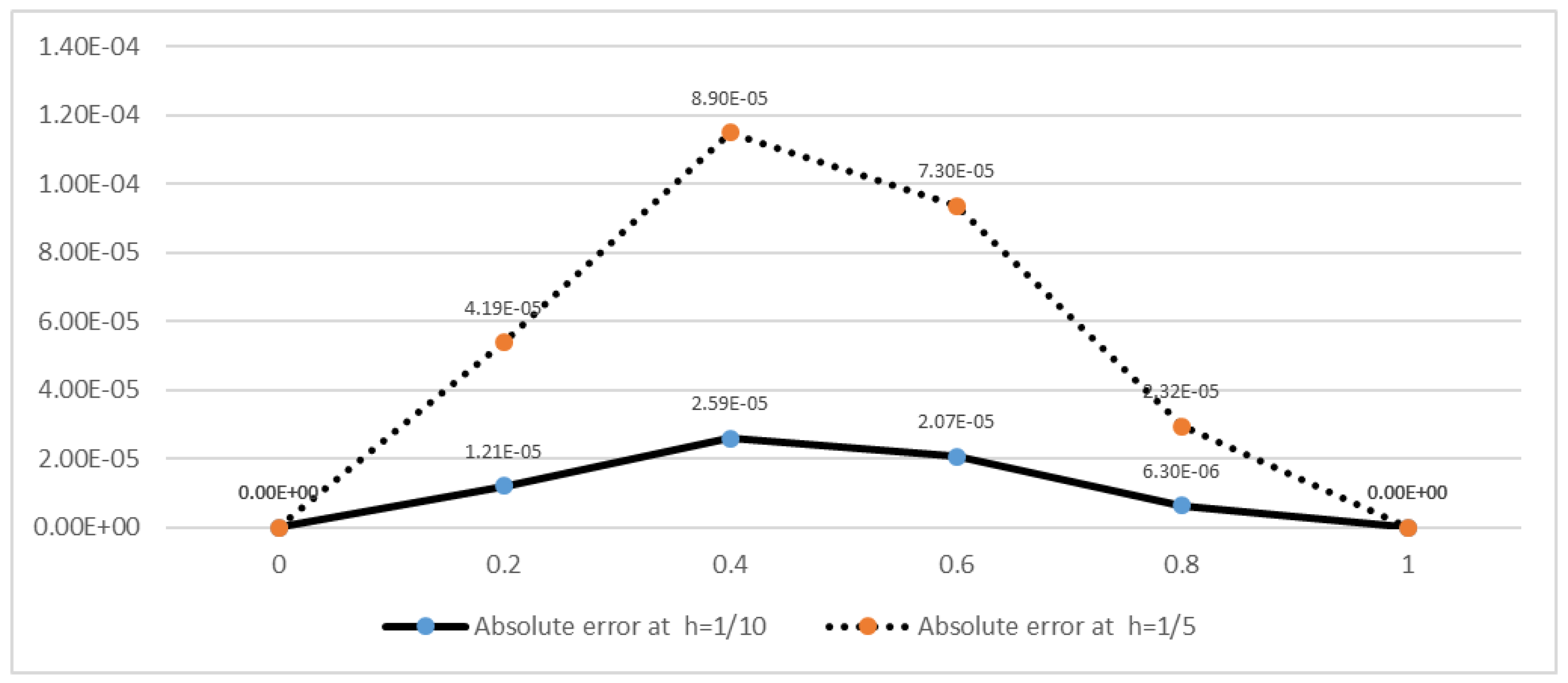
| Exact Solution | Presented Method Solution | Absolute Error | |
|---|---|---|---|
| 0 | 1 | 1 | 0 |
| 0.2 | 0.81873075307798 | 0.81877264048934 | 4.19 |
| 0.4 | 0.67032004603564 | 0.67040909568859 | 8.90 |
| 0.6 | 0.54881163609403 | 0.54888461796220 | 7.30 |
| 0.8 | 0.44932896411722 | 0.44935216696161 | 2.32 |
| 1 | 0.36787944117144 | 0.36787944117144 | 0 |
| z | Cubic B-Spline Solution of | Exact Solution of | Absolute Error of | Exact Solution of | Cubic B-Spline Solution of | Absolute error of | Exact Solution of | Cubic B-Spline Solution of | Absolute Error of |
|---|---|---|---|---|---|---|---|---|---|
| 0 | 1 | 1 | 0 | 1 | 1 | 0 | 1 | 1 | 0 |
| 0.1 | −0.9047 | −0.90477 | 6.80 | 0.9048 | 0.90461 | 2.26 | −0.9048 | −0.90973 | 4.89 |
| 0.2 | −0.8185 | −0.81864 | 9.46 | 0.8187 | 0.81805 | 6.77 | −0.8187 | −0.8241 | 5.37 |
| 0.3 | −0.7407 | −0.74074 | 7.43 | 0.7408 | 0.73979 | 1.03 | −0.7408 | −0.74435 | 3.53 |
| 0.4 | −0.6703 | −0.6703 | 2.49 | 0.6703 | 0.66918 | 1.14 | −0.6703 | −0.6713 | 9.77 |
| 0.5 | −0.6065 | −0.60656 | 2.87 | 0.6065 | 0.60553 | 9.99 | −0.6042 | −0.60537 | 1.16 |
| 0.6 | −0.5488 | −0.54888 | 6.57 | 0.5488 | 0.54811 | 7.02 | −0.5444 | −0.54658 | 2.23 |
| 0.7 | −0.4966 | −0.49666 | 7.57 | 0.4966 | 0.49622 | 3.70 | −0.4924 | −0.4945 | 2.09 |
| 0.8 | −0.4493 | −0.44939 | 6.08 | 0.4493 | 0.44921 | 1.19 | −0.4472 | −0.44828 | 1.04 |
| 0.9 | −0.4066 | −0.4066 | 3.17 | 0.4066 | 0.40656 | 1.09 | −0.4066 | −0.40665 | 8.18 |
| 1 | −0.3678 | −0.3678 | 0 | 0.3678 | 0.3678 | 0 | −0.3678 | −0.3678 | 0 |
© 2019 by the authors. Licensee MDPI, Basel, Switzerland. This article is an open access article distributed under the terms and conditions of the Creative Commons Attribution (CC BY) license (http://creativecommons.org/licenses/by/4.0/).
Share and Cite
Khalid, A.; Naeem, M.N.; Ullah, Z.; Ghaffar, A.; Baleanu, D.; Nisar, K.S.; Al-Qurashi, M.M. Numerical Solution of the Boundary Value Problems Arising in Magnetic Fields and Cylindrical Shells. Mathematics 2019, 7, 508. https://doi.org/10.3390/math7060508
Khalid A, Naeem MN, Ullah Z, Ghaffar A, Baleanu D, Nisar KS, Al-Qurashi MM. Numerical Solution of the Boundary Value Problems Arising in Magnetic Fields and Cylindrical Shells. Mathematics. 2019; 7(6):508. https://doi.org/10.3390/math7060508
Chicago/Turabian StyleKhalid, Aasma, Muhammad Nawaz Naeem, Zafar Ullah, Abdul Ghaffar, Dumitru Baleanu, Kottakkaran Sooppy Nisar, and Maysaa M. Al-Qurashi. 2019. "Numerical Solution of the Boundary Value Problems Arising in Magnetic Fields and Cylindrical Shells" Mathematics 7, no. 6: 508. https://doi.org/10.3390/math7060508
APA StyleKhalid, A., Naeem, M. N., Ullah, Z., Ghaffar, A., Baleanu, D., Nisar, K. S., & Al-Qurashi, M. M. (2019). Numerical Solution of the Boundary Value Problems Arising in Magnetic Fields and Cylindrical Shells. Mathematics, 7(6), 508. https://doi.org/10.3390/math7060508