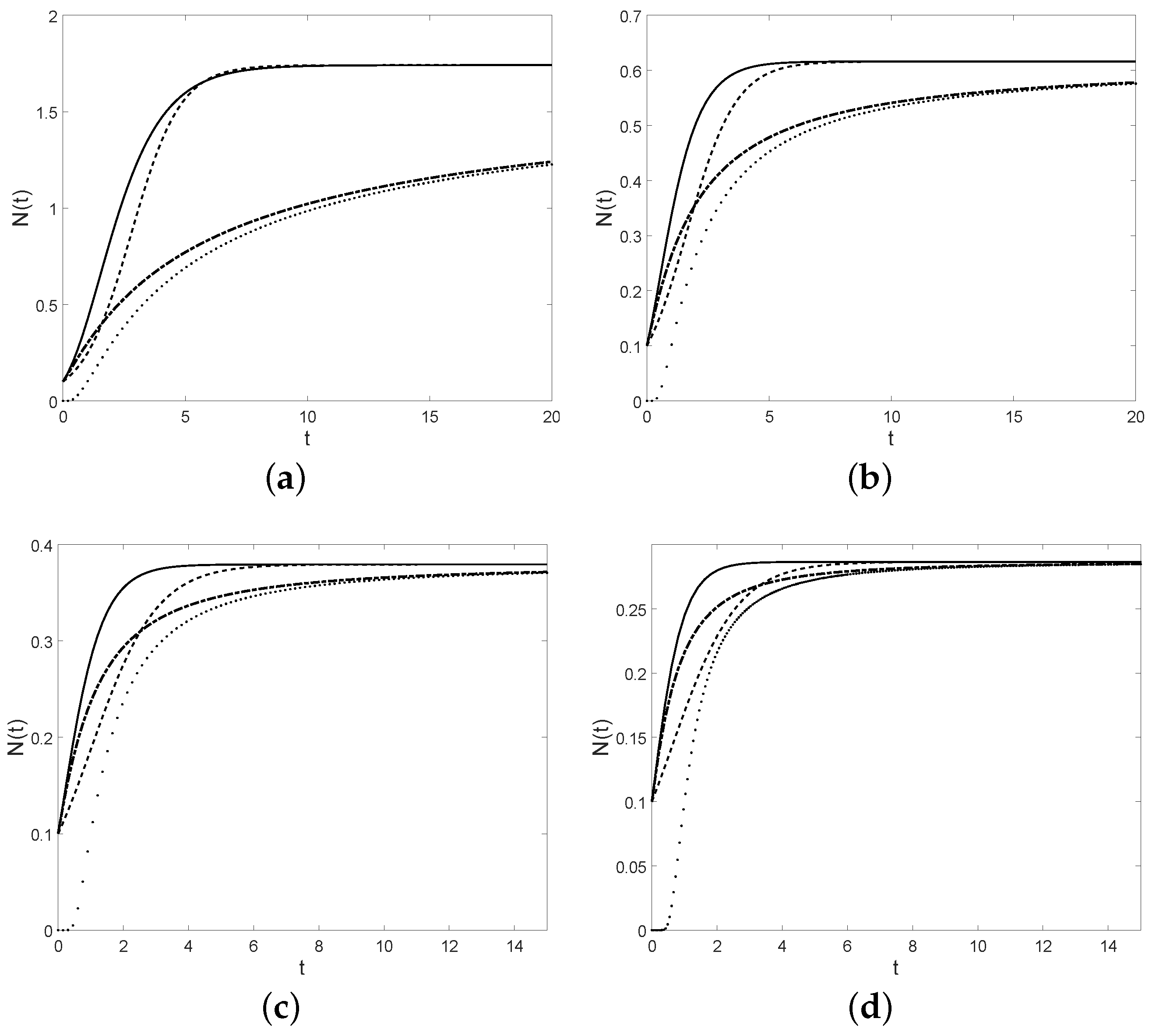
Figure 1.
Gompertz-like curve (full), Korf curve (dotted), modified Korf curve (dot-dashed), and the logistic curve N (dashed), for , , , , (a) and , (b) and , (c) and , (d) and .
Figure 1.
Gompertz-like curve (full), Korf curve (dotted), modified Korf curve (dot-dashed), and the logistic curve N (dashed), for , , , , (a) and , (b) and , (c) and , (d) and .
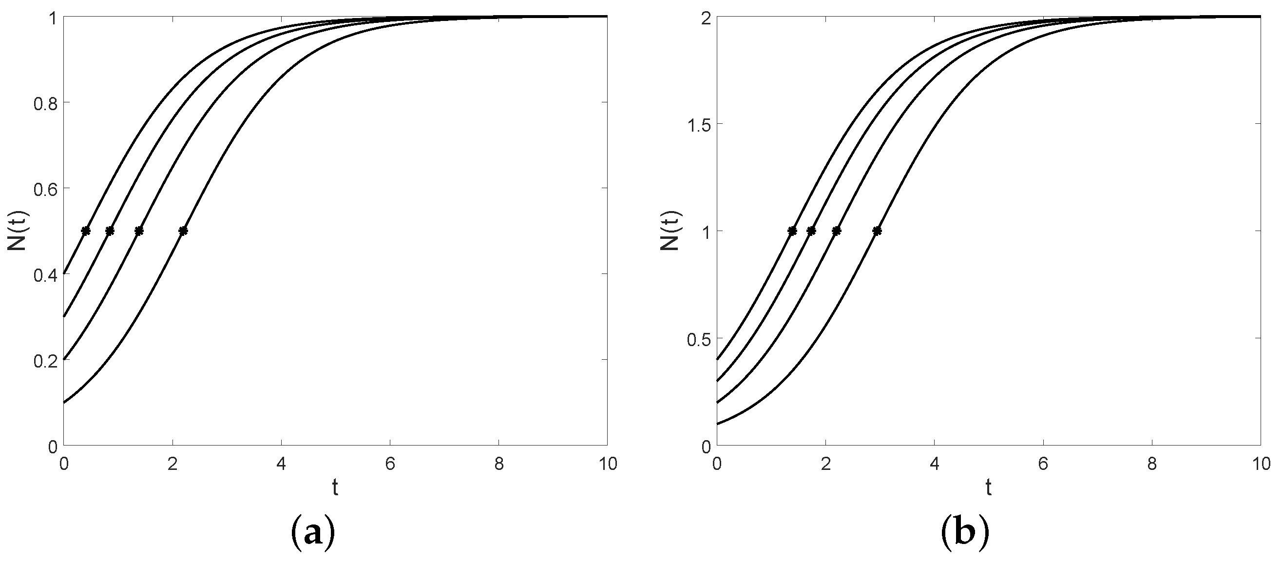
Figure 2.
The logistic function with , (a): , (bottom) and (top); (b): , (bottom) and (top).
Figure 2.
The logistic function with , (a): , (bottom) and (top); (b): , (bottom) and (top).
Figure 3.
The logistic curve and the inflection point (asterisk point) for (a) , (b) , and , respectively.
Figure 3.
The logistic curve and the inflection point (asterisk point) for (a) , (b) , and , respectively.
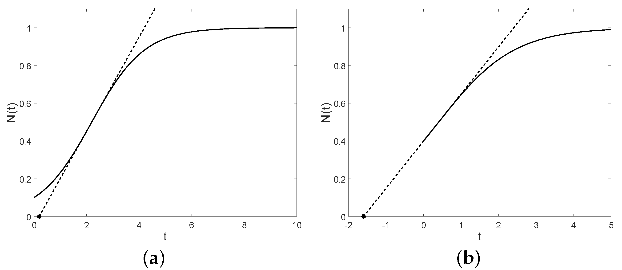
Figure 4.
The tangent lines (dashed) and the lag times (asterisk points) with , , and (a) , (b) .
Figure 4.
The tangent lines (dashed) and the lag times (asterisk points) with , , and (a) , (b) .
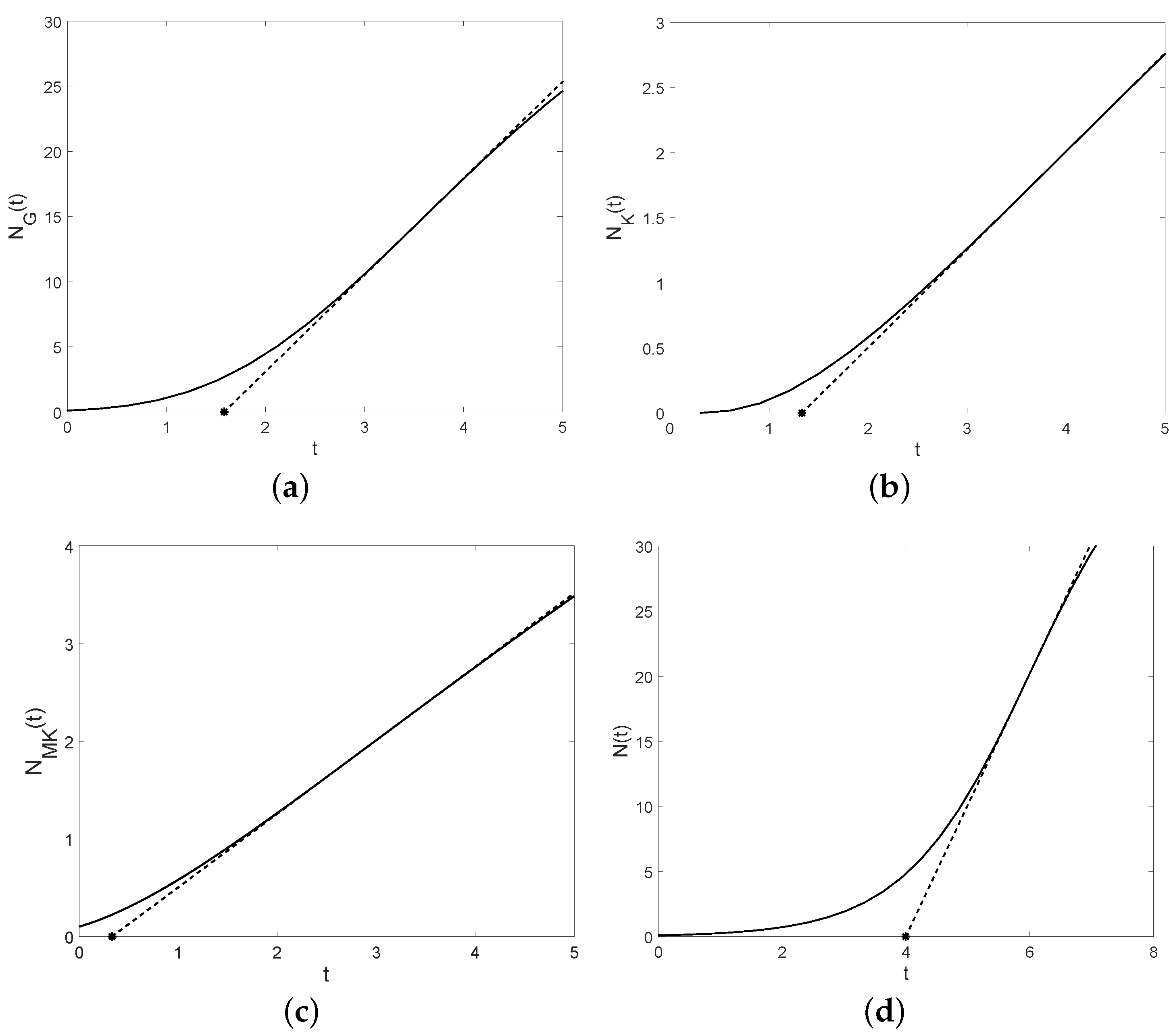
Figure 5.
The tangent lines (dashed lines) and the lag times (asterisk points) with , , , , , and for (a) Gompertz model, (b) Korf model, (c) modified Korf model, (d) logistic model.
Figure 5.
The tangent lines (dashed lines) and the lag times (asterisk points) with , , , , , and for (a) Gompertz model, (b) Korf model, (c) modified Korf model, (d) logistic model.
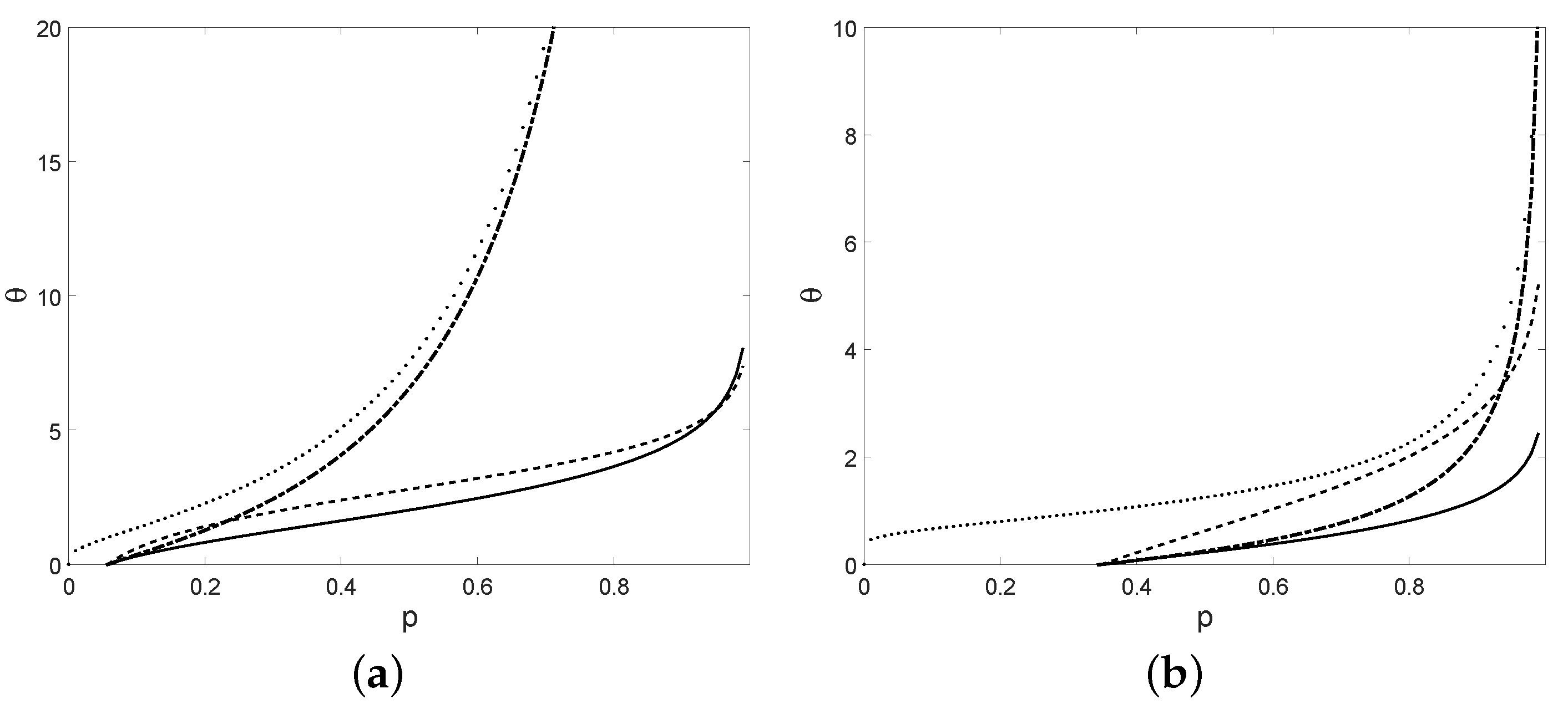
Figure 6.
The threshold crossing times (solid), (dotted), (dot-dashed), and (dashed) with , , , , (a) and , (b) and .
Figure 6.
The threshold crossing times (solid), (dotted), (dot-dashed), and (dashed) with , , , , (a) and , (b) and .
Figure 7.
Probabilities (
a):
and (
b):
, with
,
,
,
and
, with references to the cases specified in
Table 6 (case (a): full line, case (b): dashed line, case (c): dotted line, case (d): dot-dashed line).
Figure 7.
Probabilities (
a):
and (
b):
, with
,
,
,
and
, with references to the cases specified in
Table 6 (case (a): full line, case (b): dashed line, case (c): dotted line, case (d): dot-dashed line).
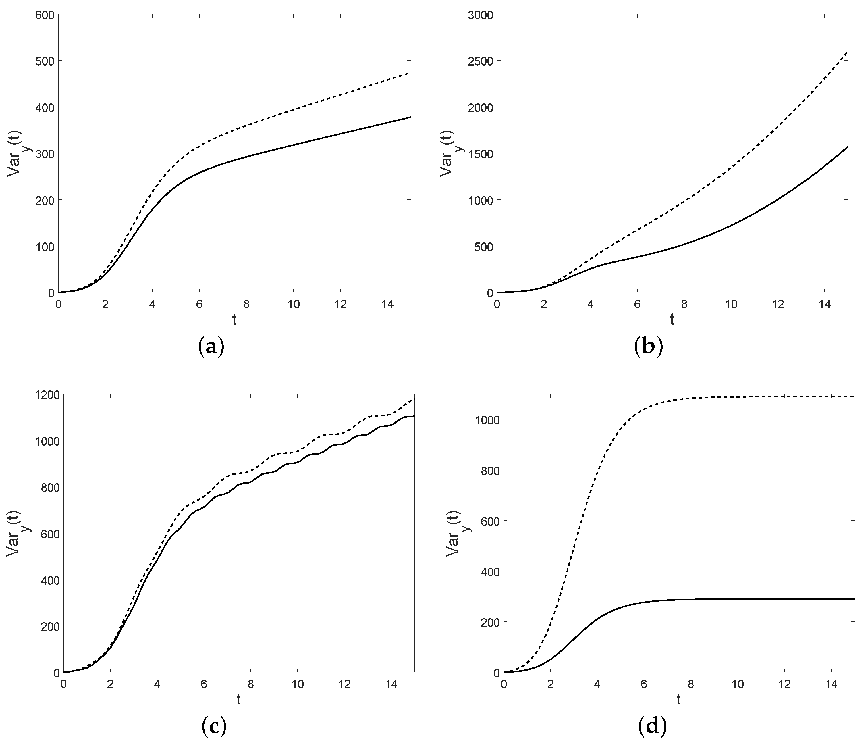
Figure 8.
For
,
, the variance
is plotted for the cases of
Table 6. In case (
a):
(solid) and
(dashed). In case (
b):
,
,
(solid) and
(dashed). In case (
c):
,
,
(solid) and
(dashed). In case (
d):
(solid) and
(dashed).
Figure 8.
For
,
, the variance
is plotted for the cases of
Table 6. In case (
a):
(solid) and
(dashed). In case (
b):
,
,
(solid) and
(dashed). In case (
c):
,
,
(solid) and
(dashed). In case (
d):
(solid) and
(dashed).
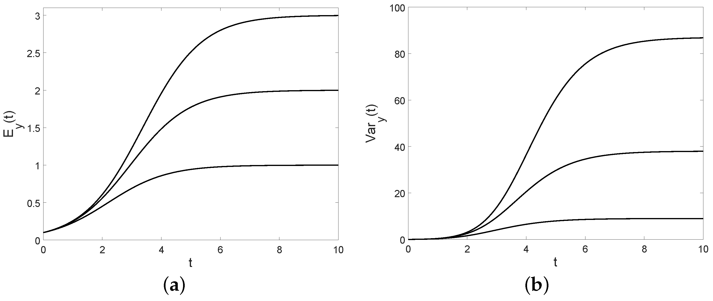
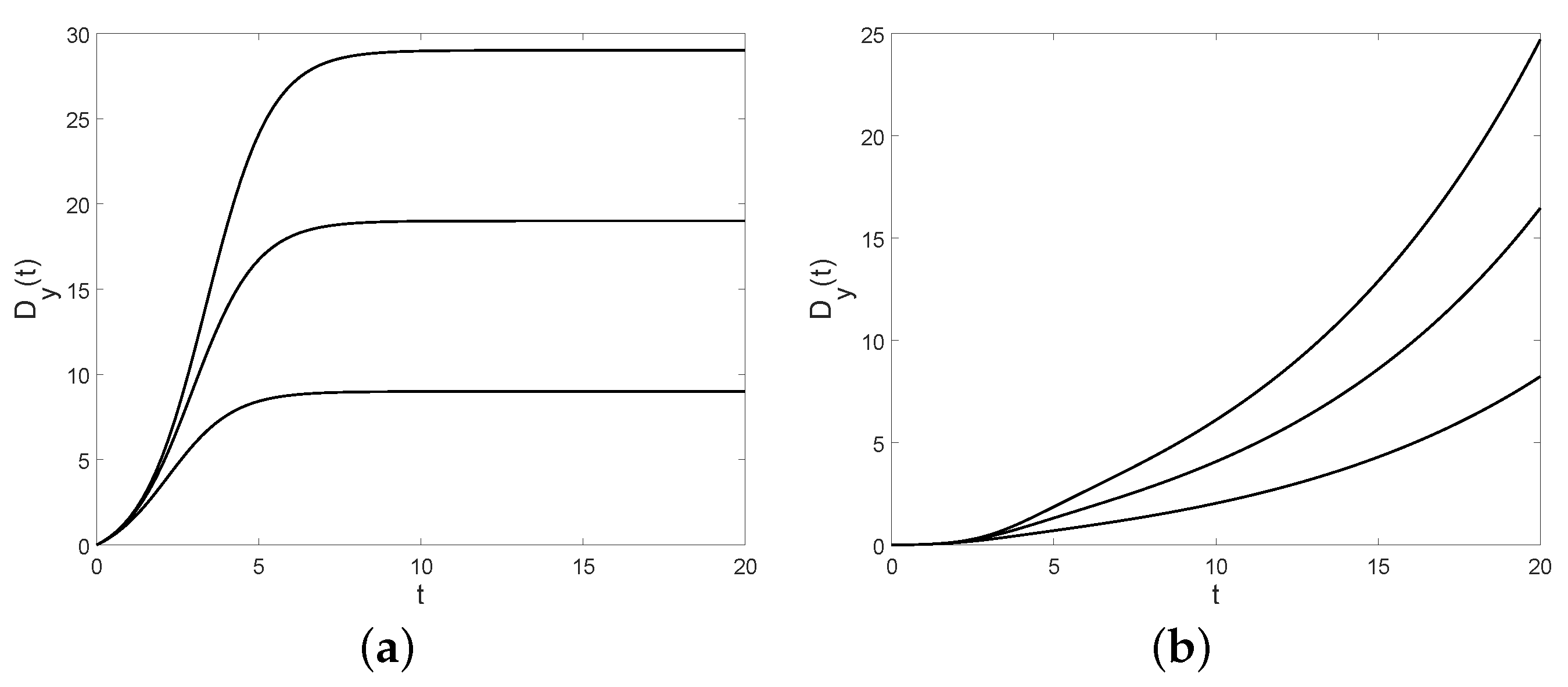
Figure 9.
(
a): The conditional mean (
26) and (
b): the conditional variance (
28) are plotted for
,
, and
(from bottom to top). For the variance the limits are 9, 38, 87, respectively.
Figure 9.
(
a): The conditional mean (
26) and (
b): the conditional variance (
28) are plotted for
,
, and
(from bottom to top). For the variance the limits are 9, 38, 87, respectively.
Figure 10.
The coefficient of variation is plotted for and (a): and (from bottom to top); (b): and (from top to bottom).
Figure 10.
The coefficient of variation is plotted for and (a): and (from bottom to top); (b): and (from top to bottom).
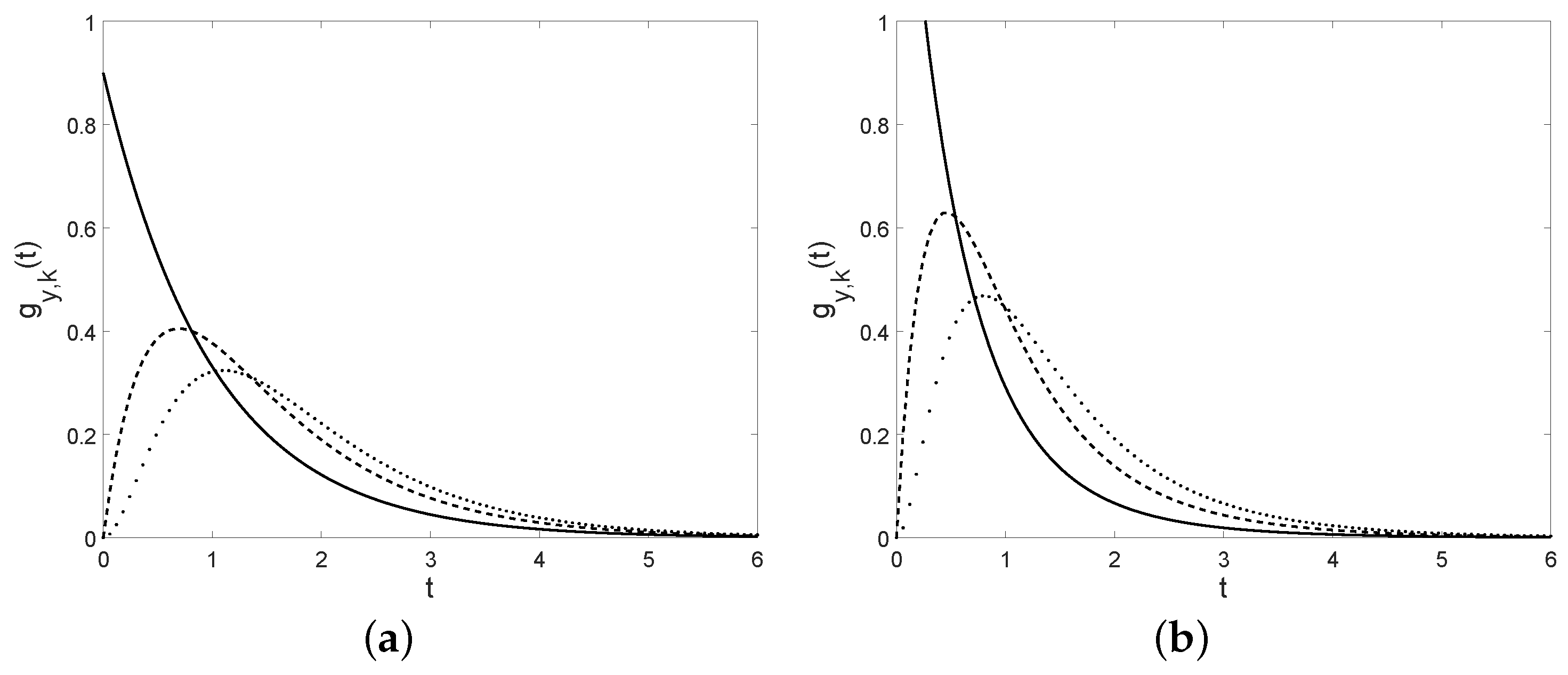
Figure 11.
The probability density function of for , , (a): (solid), (dashed), (dotted) and ; (b): (solid), (dashed), (dotted) and .
Figure 11.
The probability density function of for , , (a): (solid), (dashed), (dotted) and ; (b): (solid), (dashed), (dotted) and .
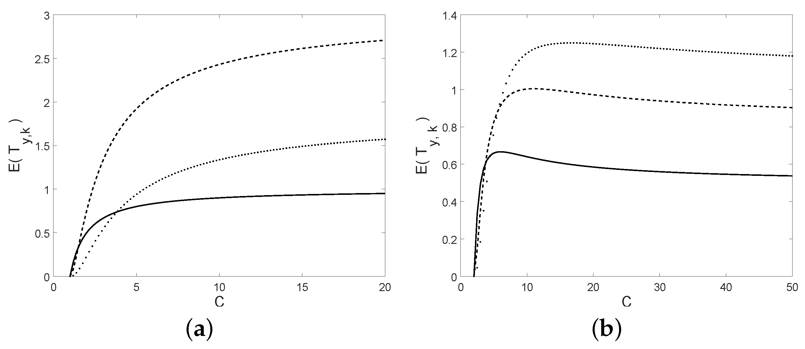
Figure 12.
The mean of is plotted as a function of C; (a): for and (solid), (dotted), (dashed); (b): for and (solid), (dashed), (dotted).
Figure 12.
The mean of is plotted as a function of C; (a): for and (solid), (dotted), (dashed); (b): for and (solid), (dashed), (dotted).
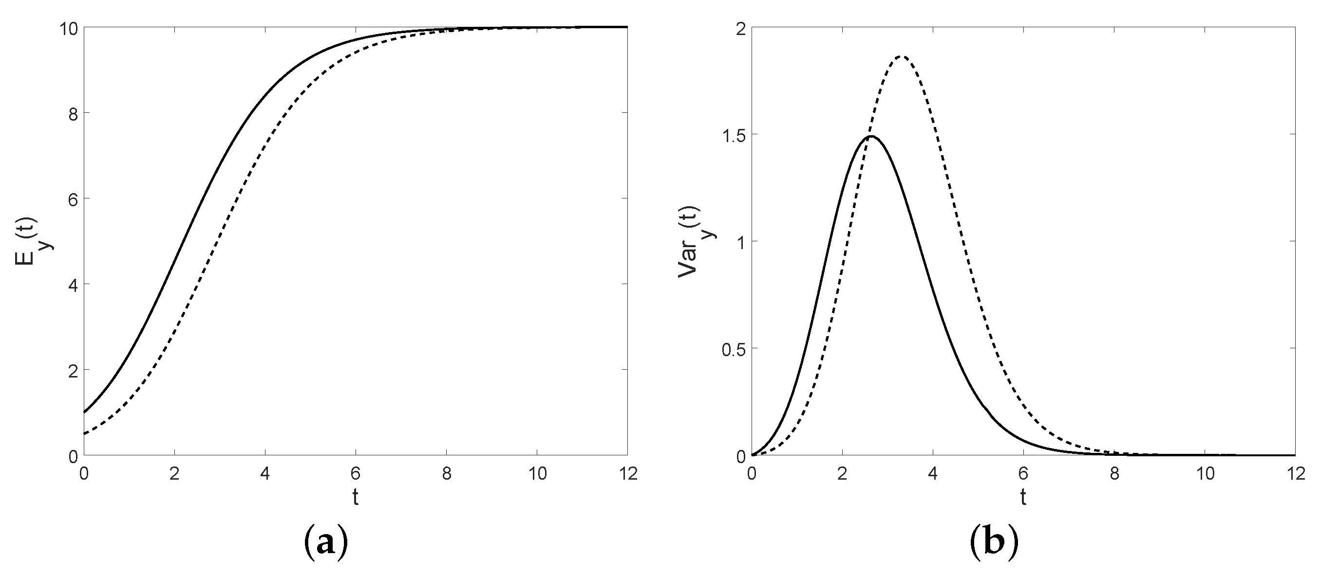
Figure 13.
The conditional mean (a) and the conditional variance (b) for , , and (solid line), (dashed line).
Figure 13.
The conditional mean (a) and the conditional variance (b) for , , and (solid line), (dashed line).
Figure 14.
Fano factor (a) and the coefficient of variation (b) are plotted for , , and (solid line), (dashed line).
Figure 14.
Fano factor (a) and the coefficient of variation (b) are plotted for , , and (solid line), (dashed line).
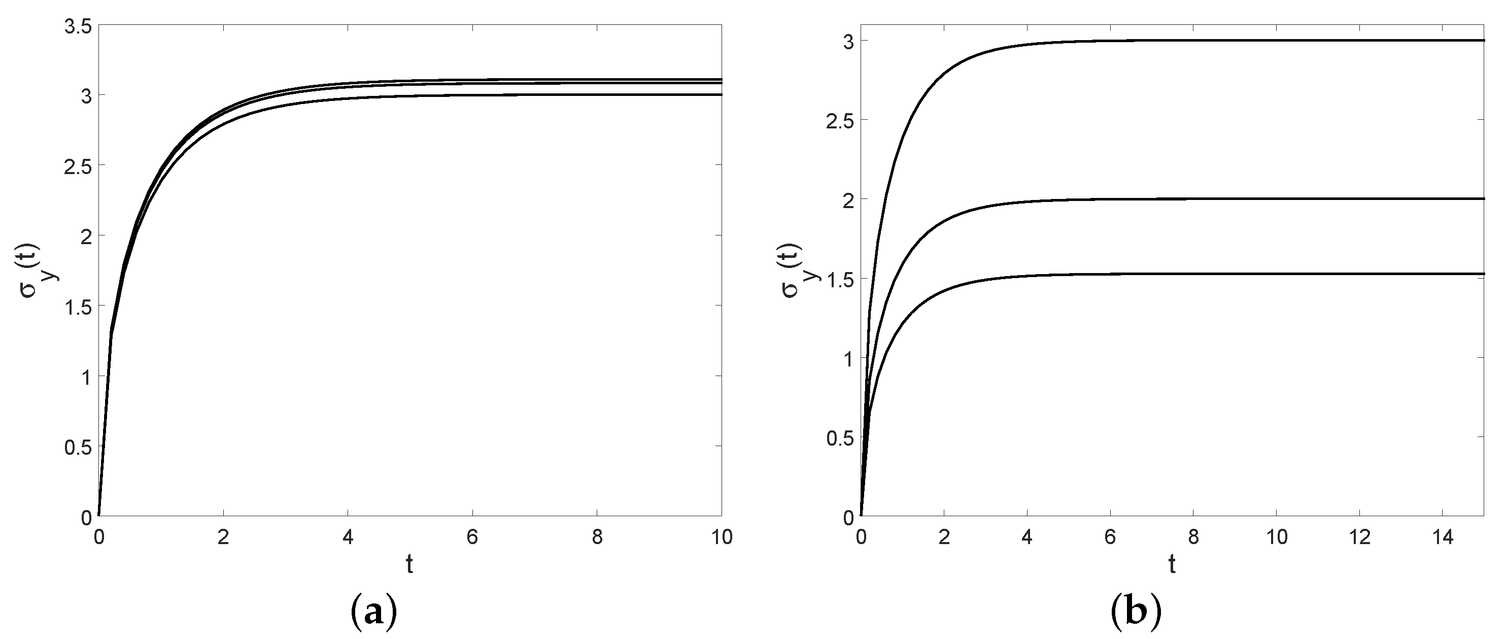
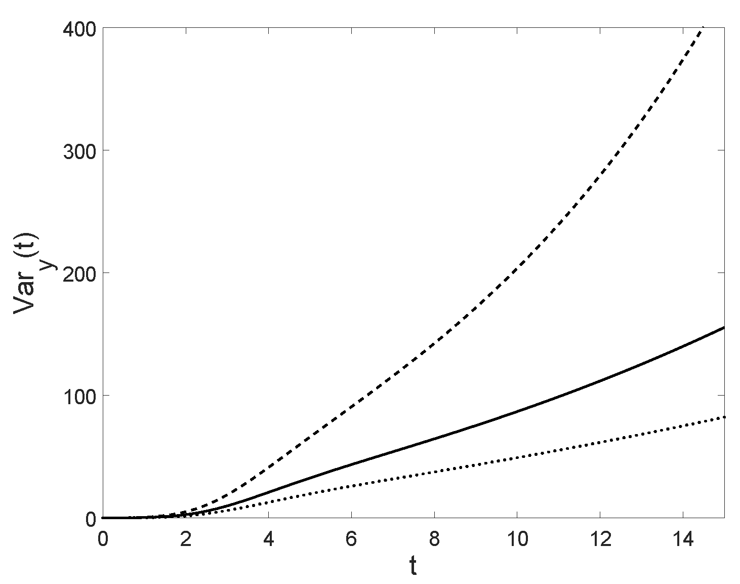
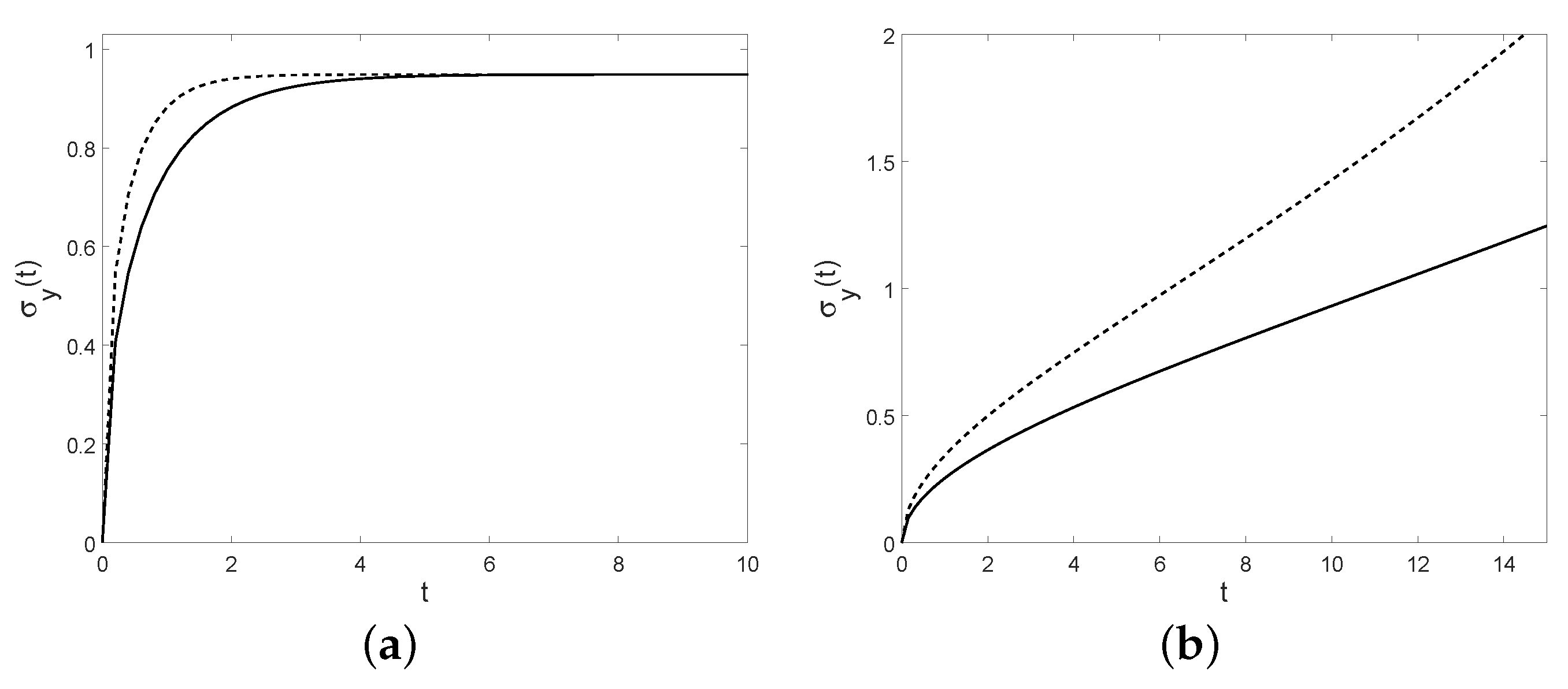
Figure 15.
For , , the conditional variance is plotted for (solid line), (dashed line) and (dotted line). Note that it is increasing with the respect to .
Figure 15.
For , , the conditional variance is plotted for (solid line), (dashed line) and (dotted line). Note that it is increasing with the respect to .
Figure 16.
For , and , the Fano factor is plotted for the birth process in (a) and for the diffusion process in (b) with (from bottom to top).
Figure 16.
For , and , the Fano factor is plotted for the birth process in (a) and for the diffusion process in (b) with (from bottom to top).
Figure 17.
For , the coefficient of variation is plotted for the birth process in (a) with (solid line) and (dashed line) and for the diffusion process in (b) with (solid line) and for (dashed line).
Figure 17.
For , the coefficient of variation is plotted for the birth process in (a) with (solid line) and (dashed line) and for the diffusion process in (b) with (solid line) and for (dashed line).
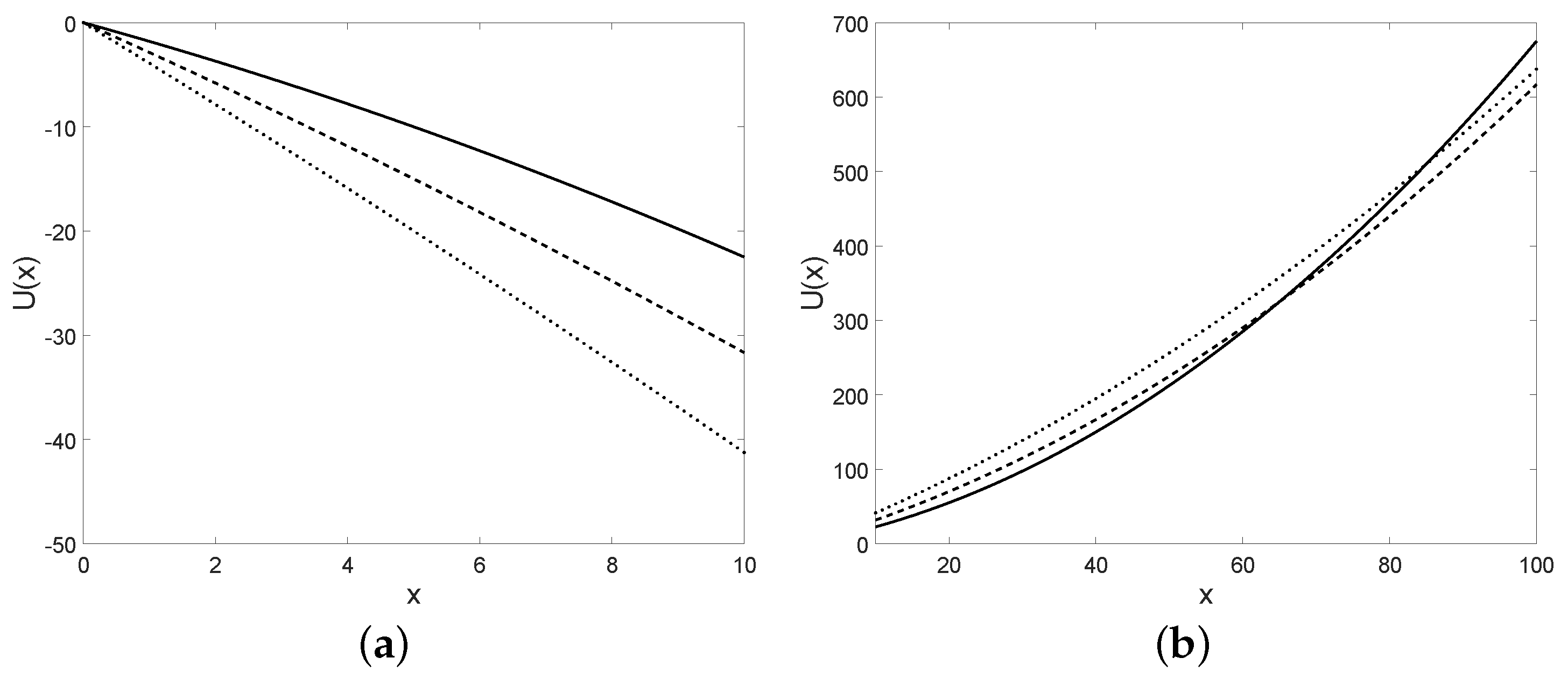
Figure 18.
The potential is plotted for in (a) and for in (b) and for , , , (solid line), (dashed line), (dotted line), with the initial condition .
Figure 18.
The potential is plotted for in (a) and for in (b) and for , , , (solid line), (dashed line), (dotted line), with the initial condition .
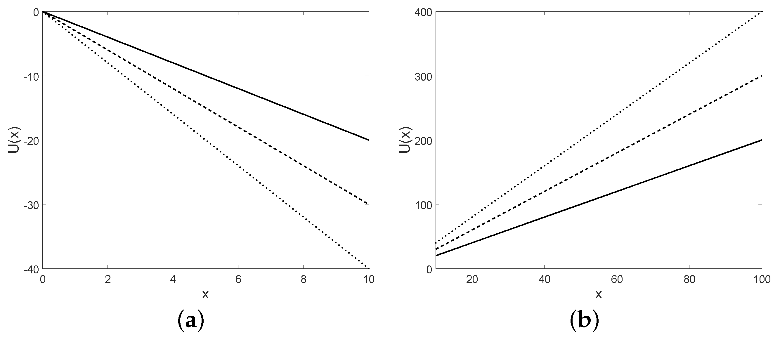
Figure 19.
The potential is plotted for in (a) and for in (b) and for , , and (solid line), (dashed line), (dotted line), with the initial condition .
Figure 19.
The potential is plotted for in (a) and for in (b) and for , , and (solid line), (dashed line), (dotted line), with the initial condition .
Table 1.
Some choices of the time-dependent growth rate and the corresponding growth curves. Parameters and are positive constants. For Gompertz-like and modified Korf models, the quantity represents the initial size of the population (), whereas for Korf model A is a positive constant and the initial size is 0.
| Model | | |
|---|
| Gompertz-like | | |
| Korf | | |
| modified Korf | | |
Table 2.
Some characteristics of the growth models.
Table 2.
Some characteristics of the growth models.
| Model | | | |
|---|
| Gompertz-like | y | | |
| Korf | 0 | 0 | |
| modified Korf | y | | |
| logistic | y | | C |
Table 3.
The inflection points and the population sizes at these points are shown for the four models.
Table 3.
The inflection points and the population sizes at these points are shown for the four models.
| Model | Inflection Point | Population at the Inflection Point |
|---|
| Gompertz-like | for | |
| Korf | | |
| modified Korf | for | |
| logistic | for | |
Table 4.
The maximum specific growth rate, the intercept of the tangent line and the lag time for the considered growth models.
Table 4.
The maximum specific growth rate, the intercept of the tangent line and the lag time for the considered growth models.
| | Intercept of Tangent Line | |
|---|
| Gompertz-like | | | |
| Korf | | | |
| modified Korf | | | |
| logistic | | | |
Table 5.
The threshold crossing times for the considered growth models.
Table 5.
The threshold crossing times for the considered growth models.
| |
|---|
| Gompertz-like | with |
| Korf | with |
| Modified Korf | with |
| Logistic | with |
Table 6.
Some choices of and the corresponding extinction probabilities. Parameters A, B, Q, and are positive constants.
Table 6.
Some choices of and the corresponding extinction probabilities. Parameters A, B, Q, and are positive constants.
| Case | | |
|---|
| (a) | A | 1 |
| (b) | | 1 |
| (c) | | 1 |
| (d) | | |
Table 7.
Some comparisons between the simple birth process of
Section 4 and the diffusion process with infinitesimal moments (
49).
Table 7.
Some comparisons between the simple birth process of
Section 4 and the diffusion process with infinitesimal moments (
49).
| Simple Birth Process | Diffusion Process |
|---|
| |
| |
| |
| |
Table 8.
The infinitesimal moments of the diffusion processes considered in
Section 5.
Table 8.
The infinitesimal moments of the diffusion processes considered in
Section 5.
| Model | Drift | Infinitesimal Variance |
|---|
| | |
| | |
| | |


