Article

Change Point Detection for Airborne Particulate Matter (PM2.5, PM10) by Using the Bayesian Approach

by
Muhammad Rizwan Khan
1 and
Biswajit Sarkar
2,*
1
Department of Industrial Engineering, Hanyang University, 222 Wangsimni-Ro, Seoul 133-791, Korea
2
Department of Industrial & Management Engineering, Hanyang University, Ansan, Gyeonggi-do 15588, Korea
*
Author to whom correspondence should be addressed.
Mathematics 2019, 7(5), 474; https://doi.org/10.3390/math7050474
Submission received: 28 February 2019 / Revised: 25 April 2019 / Accepted: 8 May 2019 / Published: 24 May 2019

Abstract

:
Airborne particulate matter (PM) is a key air pollutant that affects human health adversely. Exposure to high concentrations of such particles may cause premature death, heart disease, respiratory problems, or reduced lung function. Previous work on particulate matter ( P M 2.5 and P M 10 ) was limited to specific areas. Therefore, more studies are required to investigate airborne particulate matter patterns due to their complex and varying properties, and their associated ( P M 10 and P M 2.5 ) concentrations and compositions to assess the numerical productivity of pollution control programs for air quality. Consequently, to control particulate matter pollution and to make effective plans for counter measurement, it is important to measure the efficiency and efficacy of policies applied by the Ministry of Environment. The primary purpose of this research is to construct a simulation model for the identification of a change point in particulate matter ( P M 2.5 and P M 10 ) concentration, and if it occurs in different areas of the world. The methodology is based on the Bayesian approach for the analysis of different data structures and a likelihood ratio test is used to a detect change point at unknown time (k). Real time data of particulate matter concentrations at different locations has been used for numerical verification. The model parameters before change point ( θ ) and parameters after change point ( λ ) have been critically analyzed so that the proficiency and success of environmental policies for particulate matter ( P M 2.5 and P M 10 ) concentrations can be evaluated. The main reason for using different areas is their considerably different features, i.e., environment, population densities, and transportation vehicle densities. Consequently, this study also provides insights about how well this suggested model could perform in different areas.

1. Introduction

Airborne particulate matter is one of the most dangerous air pollutants and harmful to human health. For the last two decades, information about the negative impacts of P M 10 (particles less than 10 μ m in diameter) and P M 2.5 (particles less than 2.5 micrometers in diameter) has increased enormously. Exposure to high concentrations of such particles may cause premature death, heart disease, respiratory problems, or reduced lung function through different mechanisms, which include pulmonary and systemic inflammation, accelerated atherosclerosis, and altered cardiac autonomic function (Heroux et al. [1] and Pope et al. [2]). Therefore, to control particulate matter (PM) pollution, and to make effective plans for counter measurements, it is important to measure the efficiency and effectiveness of policies applied by the Ministry of Environment. Every region has developed different kinds of extensive bodies of legislation, which establish air quality standards for key air pollutants to improve the air quality and to satisfy these standards. The European Environment Agency, the United States Environmental Protection Agency, and the Ministry of Environment in South Korea have each set their own air quality standards for all air pollutants. Thus, It is essential to follow established air quality monitoring systems to measure the PM concentrations on an hourly as well as daily basis, because some areas deviate from the established PM standards. This may cause adverse environmental effects and serious health problems.
Until now, a number of statistical methods have been established to model the hazards of PM from air quality standards. A Bayesian multiple change point model was proposed to measure the quantitative efficiency of pollution control programs for air quality, which estimate the hazards of different air pollutants. In the model, it was assumed as a nonhomogeneous Poisson process with multiple change points. The change points were identified, and a rate function was estimated by using a reversible jump MCMC algorithm (Gyarmati-Szabo et al. [3]). In another study, the changes in health effects due to simultaneous exposure to physical and chemical properties of airborne particulate matter were gauged through Bayesian approach and inferences were drawn via the Markov Chain Monte Carlo method (Pirani et al. [4]). A Bayesian approach was introduced to estimate the distributed lag functions in time series models, which can be used to determine the short-term health effects of particulate air pollution on mortality (Welty et al. [5]). Hybrid models were proposed to forecast the PM concentrations for four major cities of China; Beijing, Shanghai, Guangzhou, and Lanzhou (Qin et al. [6]).
A change point detection method for detecting changes in the mean of the one dimensional Gaussian process was proposed on the basis of a generalized likelihood ratio test (GLRT). The important characteristic of this method is that it includes data dependence and covariance of the Gaussian process. However, in case of unidentified covariance, the plug-in GLRT method was suggested which remains asymptotically near optimal (Keshavarz et al. [7]). A new method for acute change point detection was proposed for fractional Brownian motion with a time dependent diffusion coefficient. The likelihood ratio method has been used for change point detection in Brownian motion. A statistical test was also suggested to identify the significance of a calculated critical point (Kucharczyk et al. [8]). The change point detection technique in machine monitoring was suggested, which was based on two stages. In the first stage, irregularities are measured in time series data through the automatic regression (AR) model, and then the martingale statistical test is applied to detect the change point in unsupervised time series data (Lu et al. [9]). An integrated inventory model was developed to determine the optimal lot size and production uptime while considering stochastic machine breakdown and multiple shipments for a single-buyer and single-vendor (Taleizadeh et al. [10]).
A statistical change point algorithm based on nonparametric deviation estimation between time series samples from two retrospective segments was proposed in which the direct density ratio estimation method was applied for deviation measurement through relative Pearson divergence (Liu et al. [11]). A novel statistical methodology for online change point detection was suggested in which data for an uncertain system was composed through an autoregressive model. On the basis of nonparametric estimation of unidentified elements, an innovative CUSUM-like scheme was recommended for change detection. This estimation method could also be updated online (Hilgert et al. [12]). A new methodology, the Karhunen-Loeve expansions of the limit Gaussian processes, was suggested for change point test in the level of a series. Firstly, change point detection in the mean was explained, which later extended to linear and nonlinear regression (Górecki et al. [13]). A Cramer-von Mises type test was presented to test the sudden changes in random fields which was dependent on Hilbert space theory (Bucchia and Wendler [14]). The continuous-review inventory model was developed for Controllable lead time for comparing two models; one with normally distributed lead time demand and the second assumes that there is no specific distribution for lead time demand (Shin et al. [15]).
A new technique was developed to identify the structural changes in linear quantile regression models. When a structural change in the relationship between covariates and response at a specific point exists, it may not be at the centre of response distribution, but at the tail. The traditional mean regression method might not be applicable for change point detection of such structural changes at tails. Subsequently, the proposed technique could be appropriate for it (Zhou et al. [16]). For detection of simultaneous changes in mean and variance, a new methodology called the fuzzy classification maximum likelihood change point (FCML-CP) algorithm was suggested. Multiple change points in the mean and variance of a process can be estimated by this method. This technique is much better than the normal statistical mixture likelihood method because it saves a lot of time (Lu and Chang [17]). A model for Partial Trade-Credit Policy of Retailer was developed in which deterioration of products was assumed as exponentially distributed (Sarkar and Saren [18]).
The Bayesian change point algorithm for sequential data series was introduced which has some uncertain limitations regarding location and number of change points. This algorithm was precisely based on posterior distribution to deduce if a change point has occurred or not. It can also update itself linearly as new data points are observed. Posterior distribution monitoring is the finest way to identify the presence of a new change point in observed data points. Simulation studies illustrate that this algorithm is good for rapid detection of existing change points, and it is also known for a low rate of false detection (Ruggieri and Antonellis [19]). Due to the probabilistic concept of Bayesian change point detection (BCPD), this methodology can overcome threats in identifying the location and number of change points.
The performance of two different methods for change point detection of multivariate data with both single and multiple changes was compared. The results illustrated adequate performance for both Expectation Maximization (EM) and Bayesian methods. However, EM exhibits better performance in case of minor changes and unsuitable priors while the Bayesian method has less computational work to do (Keshavarz and Huang [20]). The Bayesian multiple change point model was suggested for the identification of Distributed Denial of Service (DDoS) flooding attacks in VoIP systems in which Session Initiation Protocol (SIP) is used as signalling mechanism (Kurt et al. [21]). One of the well-known change detection techniques is post classification with multi temporal remote sensing images. An innovative post classification technique with iterative slow feature analysis (ISFA) and Bayesian soft fusion was suggested to acquire accurate and reliable change detection maps. Three steps were suggested in this technique, first was to get the class probability of images through independent classification. After that, a continuous change probability map of multi temporal images was obtained by ISFA algorithm. Lastly, posterior probabilities for the class combinations of coupled pixels were determined through the Bayesian approach to assimilate the class probability with the change probability, which is called Bayesian soft fusion. This technique could be widely applicable in land cover monitoring and change detection at a large scale (Wu et al. [22]).
The Bayesian change point technique was designed to analyse biomarkers time series data in women for the diagnosis of ovarian cancer. The identification of such kind of change points could be used to diagnose the disease earlier (Mariño et al. [23]). The Generalized Extreme Value (GEV) fused lasso penalty function was applied to identify the change point of annual maximum precipitation (AMP) in South Korea. Numerical analysis and applied data analysis were conducted in order to compare performance from the GEV fused lasso and Bayesian change point analysis, which shows that when water resource structures are hydrologically designed the GEV fused lasso method should be used to identify the change points (Jeon et al. [24]). The Bayesian method was recommended to identify the change point occurrence in extreme precipitation data, and the model follows a generalized Pareto distribution. This Bayesian change point detection was inspected for four different situations, one with no change model, second with a shape change model, third with a scale change model, and fourth with both a scale and shape change model. It was determined that unexpected and sustained change points need to be considered in extreme precipitation while making hydraulic design (Chen et al. [25]).
Bayesian change point methodology was presented to identify changes in the temporal event rate for a non-homogeneous Poisson process. This methodology was used to determine if a change in the event rate has occurred or not, the time for change, and the event rate before or after the change. The methodology has been explained through an example of earthquake occurrence in Oklahoma. This spatiotemporal change point methodology can also be used for identifying changes in climate patterns and assessing the spread of diseases. It permits participants to make real time decisions about the influence of changes in event rates (Gupta and Baker [26]). A new Bayesian methodology was recommended to analyze multiple time series with the objective of identifying abnormal regions. A general model was developed and it was shown that Bayesian inference allows independent sampling from the posterior distribution. Copy number variations (CNVs) are identified by using data from multiple individuals. The Bayesian method was evaluated on both real and simulated CNV data to provide evidence that this method is more precise as compare to other suggested methods for analyzing such data (Bardwell and Fearnhead [27]).
All the above mentioned methods are either too complex and complicated for application on random hazards of PM or not applicable to randomness of PM hazards. Therefore, still more studies are required to investigate the PM hazards, due to its complex and varying properties and associated ( P M 10 and P M 2.5 ) concentrations and compositions, to investigate the numerical productivity of pollution control programs for air quality. The primary purpose of this research is to develop models for change point detection of particulate matter ( P M 2.5 and P M 10 ) concentrations if it occurs in different areas. The pollutant concentrations before and after a change point has to be critically analyzed so that the proficiency and success of environmental policies for particulate matter ( P M 2.5 and P M 10 ) concentrations can be evaluated. The Bayesian approach is used to analyze random hazards of PM concentrations with a change point at an unknown time (k).
To demonstrate the proposed approach, real time data of random hazards of PM concentrations at different sites has been used. The PM concentrations change point (k), parameters before change point ( θ ), and parameters after change point ( λ ) have been comprehensively analyzed by using the Bayesian technique. Thus, simulation models have been constructed for different data structures. The main reason for using different areas is their considerably different features i.e., environment, population densities, and transportation vehicle densities. Consequently, this study also provides insight about how well this suggested model could perform in different areas. The paper is structured as follows: Section 2 refers to problem definitions, explaining assumptions along with notation, and Section 3 shows the formulation of mathematical models. Section 4 and Section 5 depict numerical examples and results, respectively, to validate the practical applications of the proposed models. Section 6 discusses the depicted results of previous section, it also explains the managerial insights of results. Finally, Section 7 presents conclusions of this study. Table 1 depicts the comparative study of different authors who have contributed in the direction of research, while the last row of the table portrays the contribution of this research paper. On the other hand, Table 2 and Table 3 compares the difference in previous workings and this work.

2. Problem Definition, Notation and Assumptions

2.1. Problem Definition

The major objective of this research is to develop a more precise, well defined and user friendly method for application on random hazards of PM to detect the change point of subjected air pollutant hazards at any unknown time (k) if it occurs at any area across the globe. The existing methods are either too complex and complicated for the application on random hazards of PM due to its complex and varying properties or not applicable to randomness of PM hazards. Therefore, still more studies are required to develop a such kind of methodology, which is easily understandable and appropriate to model the hazards of the PM concentrations from air quality standards that can also detect change points in these hazards. Secondly, this method could be applicable for any kind of time series and data distributions. Analysis of these changes need to be done, whether these change points are favorable or not for the environment. For this, a comparison of subjected pollutant hazards before and after a change point has to be done for the evaluation of pollution control programs adopted by environmental protection agencies. If hazards occurrences increase after the change point, then environmental policies have a negative impact which marks the failure of pollution control program, but if the hazards occurrences reduce after the change point, then it demonstrates the effectiveness of the pollution control program. Thirdly, an alteration in occurrences must be measured to define the new pollution control policies for further improvements in the current level of subjected air pollutant hazards.
For anticipated goals, the Bayesian approach will be used to determine posterior probabilities of pollutant occurrences and the likelihood ratio test will be used for identifying the change point in that Bayesian model. This suggested model would be numerically validated by using real-time data of particulate matters’ concentrations in different areas of Seoul, South Korea, observed from January 2004 to December 2013. The change point (k) for for particulate matter ( P M 2.5 and P M 10 ) hazards, the rate before the change point ( θ ), and the rate after the change point ( λ ) would be comprehensively analyzed. The central idea for using different regions is their considerably different features i.e., environment, population densities, and transportation vehicle densities. Hence, this study can also be a vision for the implementation of recommended model in different areas.Air quality standards for particular matter P M 2.5 and P M 10 are given in Table 4. Results have been determined by following these standards.
Table 5 and Table 6 illustrate some details regarding data collected for Guro, Nowon, Songpa, and Yongsan which exhibit standard-wise and location-wise percentage of polluted days. In case of P M 2.5 , more than 44%, 21% and 8% days are polluted as per European, American and Korean standards respectively, which is alarming. Similarly, in case of P M 10 , the polluted days concentrations as per European and Korean standards is more than 40% and 6% respectively and it could not be acceptable. Hence, there is a need to control hazards of PM.

2.2. Notation

The list of notation to represent the random variables and parameters is as follows:
Indices
i  
replication or sequence, i = 1, 2, …
j  
position in the chain, j = 1, 2, …n
Random variables
Y   
random process
y   
variable (Y) at any given point
y i   
variable (Y) at point i where i 0 , 1 , 2
Parameters
k  
change point in the random process
θ   
parameter before change point k associated with probability distribution function of random variable Y
λ   
parameter after change point k associated with probability distribution function of random variable Y
Variables
P r ( θ )    
prior distribution for parameter θ
P r ( θ | y i )   
posterior distribution for parameter θ
P r ( λ | y i )   
posterior distribution for parameter λ
P r ( y i | θ )   
likelihood or sampling model
V  
mean of the chain or replications (Average of daily pollutant concentrations)
V i j   
jth observation from the ith replication
V i   
mean of ith replication
V  
mean of m replications
B  
between sequence variance represents the variance of replications with the mean of m replications
S i 2   
variance for all replications
W  
within sequence variance is the mean variance for m replications
V a r ( V )   
overall estimate of the variance of V in the target distribution
R   
estimated potential scale reduction for convergence

2.3. Assumptions

The following assumptions were used for the proposed model:
  • Y represents the number of times an event occurs in time t and Y is always positive real numbers y 1 , 2 that can be any random value.
  • Y ( 0 ) = 0 means that no event occurred at time t = 0 .
  • Time series random data observed on equal interval of lengths.
  • The particulate matter daily concentrations or occurrence of events follow specific random probability distribution function.
  • The particulate matter daily concentrations in any interval of length ( t ) is a random variable and number of times event occurs is also positive random variable with parameter ( r a t e = θ ) .

3. Mathematical Model

3.1. Formulation of Mathematical Model

The probability distribution function of a random variable Y at any given point y in the sample space is given as follows:
f ( y ; θ ) = P r ( Y = y | θ ) f o r y 1 , 2
There could be a single parameter or multiple parameters depending upon the probability distribution function of random variable Y.
The change point for random process Y is being detected by the likelihood ratio test and that is a statistical test used for comparing the goodness of fit for two statistical models; one is null model and other is alternative model. The test is based on the likelihood ratio, which states how many times more likely the data are under one model than the other. This likelihood ratio compared to a critical value used to decide whether to reject the null model.
f ( Change point | Y , Eexpectation before change point , Expectation after change point ) = L Y ; Change point , Expectation before change point , Expectation after change point j = 1 n L Y ; j , Change point , Expectation before change point , Expectation after change point
and parameters’ comparison before and after the change-point is also being done.
Let the change point in the random process be denoted by k and θ be the random variable parameter before change point k while λ be the random variable parameter after change point k. It can be represented as:
y i p d f ( θ ) for i = 1 , 2 , . , k
y i p d f ( λ ) for i = k + 1 , k + 2 , , n
Hence,
f ( y ; θ ) = P r ( Y = y i | θ ) for i = 1 , 2 , . , k
f ( y ; λ ) = P r ( Y = y i | λ ) for i = k + 1 , k + 2 , , n
The joint pdf (probability density function) is the product of marginal pdf. If random variable Y = y i with parameter θ is modelled, then joint pdf of our sample data will be as below:
P r ( Y = y i | θ ) = i = 1 n P r ( y i | θ ) f o r i 0 , 1 , 2 , , n
A class of prior densities is conjugate for the likelihood/sampling model P r ( y i | θ ) if the posterior distribution is also in the same class. Therefore, prior distribution P r ( θ ) and posterior distribution P r ( θ | y i ) will follow the same conjugate prior distribution to the likelihood/sampling model P r ( y i | θ ) . However, the likelihood P r ( y i | θ ) follows the random distribution based on data. Therefore, the prior distribution P r ( θ ) of parameters and posterior distribution P r ( θ | y i ) of the same parameters must be same and conjugate for Bayesian analysis. Bayes theorem for parameter’s θ and λ is as follows:
P r ( θ | y i ) P r ( θ ) P r ( y i | θ )
P r ( λ | y i ) P r ( λ ) P r ( y i | λ )
By applying Bayes theorem, the posterior distribution of model parameters θ and λ can be determined
P r ( θ | y i ) = P r ( y i | θ ) P r ( θ ) P r ( y i ) f o r i 1 , 2 , , k
P r ( λ | y i ) = P r ( y i | λ ) P r ( λ ) P r ( y i ) f o r i k + 1 , k + 2 , , n
As,
L ( θ | Y ) = f θ ( Y ) = f ( Y | θ )
Now, apply likelihood ratio test statistic for change point detection
f ( k | Y , θ , λ ) = L Y ; k , Expectation before change point , Expectation after change point j = 1 n L Y ; j , Expectation before change point , Expectation after change point
And likelihood will be determined as given by:
L ( Y ; k , θ , λ ) = e x p k ( ( Expectation after k point Expectation before k point ) Expectation before k Expectation after k i = 1 k y i
The change point k is uniform over y i . Please note that θ , λ and k are all independent of each other.

3.1.1. Convergence of the Parameters

A single simulation run of a somewhat arbitrary length cannot represent the actual characteristics of the resulting model. Therefore, to estimate the steady-state parameters, the Gelman-Rubin Convergence diagnostic has to be applied in which target parameters are estimated by running multiple sequences of the chain. m replications of the simulation ( m 10 ) are made, each of length n = 1000 . If the target distribution is unimodal then Cowles and Carlin recommends that we must run at least ten chains, as this approach monitors the scalar numbers of interest in the analysis. Therefore, the mean rate of pollutant concentrations is a parameter of interest that is denoted by V.
Scalar summary V = Mean of the chain (Average of daily pollutant concentrations)
Let V i j be the jth observation from the ith replication
V i j , i = 1 , 2 , . , m j = 1 , 2 , . , n
Mean of ith replication
V i = 1 n j = 1 n V i j
Mean of m replications
V = 1 m i = 1 m V i
The between sequence variance represents the variance of replications with the mean of m replications calculated as follows:
B = n m 1 i = 1 m ( V i V ) 2
Variance for all replications is calculated to determine the within sequence variance
S i 2 = 1 n 1 j = 1 n ( V i j V ) 2
The within sequence variance is the mean variance for k replications determined as given below:
W = 1 m i = 1 m S i 2
Finally, the within sequence variance and between sequence variance are combined to get an overall estimate of the variance of V in the target distribution
V a r ( V ) = n 1 n W + 1 n B
Convergence is diagnosed by calculating
R = V a r ( V ) W
This factor R (estimated potential scale reduction) is the ratio between the upper and lower bound on the space range of V which is used to estimate the factor by which V a r ( V ) could be reduced through more iterations. Further iterations of the chain must be run if the potential scale reduction is high. Run the replications until R is less than 1.1 or 1.2 for all scalar summaries.

3.1.2. Flowchart

The flowchart (Figure 1) for change point k detction, for any random process Y, is given as follows:

3.2. Comparison Method for Change Point Detection

A change point analysis has been done by using a combination of CUSUM (cumulative sum control chart) and bootstrapping for comparative analysis.

3.2.1. The CUSUM (Cumulative Sum Control Chart) Technique

The CUSUM (cumulative sum control chart) is a sequential analysis technique typically used for monitoring change detection. CUSUM charts are constructed by calculating and plotting a cumulative sum based on the data. The cumulative sums are calculated as follows:
  • First calculate the average.
    X ¯ = X 1 + X 2 + X 3 + . , n
  • Start the cumulative sum at zero by setting S 0 = 0
  • Calculate the other cumulative sums by adding the difference between current value and the average to the previous sum, i.e.,
    S i = S i 1 + X i X ¯
Plot the series and the cumulative sum is not the cumulative sum of the values. Instead it is the cumulative sum of differences between the values and the average. Because the average is subtracted from each value, the cumulative sum also ends at zero.
Interpreting a CUSUM chart requires some practice. Suppose that during a period of time the values tend to be above the overall average. Most of the values added to the cumulative sum will be positive and the sum will steadily increase. A segment of the CUSUM chart with an upward slope indicates a period where the values tend to be above the overall average. Likewise a segment with a downward slope indicates a period of time where the values tend to be below the overall average. A sudden change in direction of the CUSUM indicates a sudden shift or change in the average. Periods where the CUSUM chart follows a relatively straight path indicate a period where the average did not change.

3.2.2. Bootstrap Analysis

A confidence level can be determined for the apparent change by performing a bootstrap analysis. Before performing the bootstrap analysis, an estimator of the magnitude of the change is required. One choice, which works well regardless of the distribution and despite multiple changes, is S d i f f defined as:
S d i f f = S m a x S m i n
S m a x = max i = 0 , 1 , 2 , , S i
S m i n = min i = 0 , 1 , 2 , , S i
Once the estimator of the magnitude of the change has been selected, the bootstrap analysis can be performed. A single bootstrap is performed by:
  • Generate a bootstrap sample of n units, denoted X 0 1 , X 0 2 , X 0 3 , X 0 n by randomly reordering the original n values. This is called sampling without replacement.
  • Based on the bootstrap sample, calculate the bootstrap CUSUM, denoted S 0 0 , S 0 1 , S 0 2 , S 0 n .
  • Calculate the maximum, minimum and difference of the bootstrap CUSUM, denoted S 0 m a x , S 0 m i n and S 0 d i f f .
  • Determine whether the bootstrap difference S 0 d i f f is less than the original difference S d i f f .
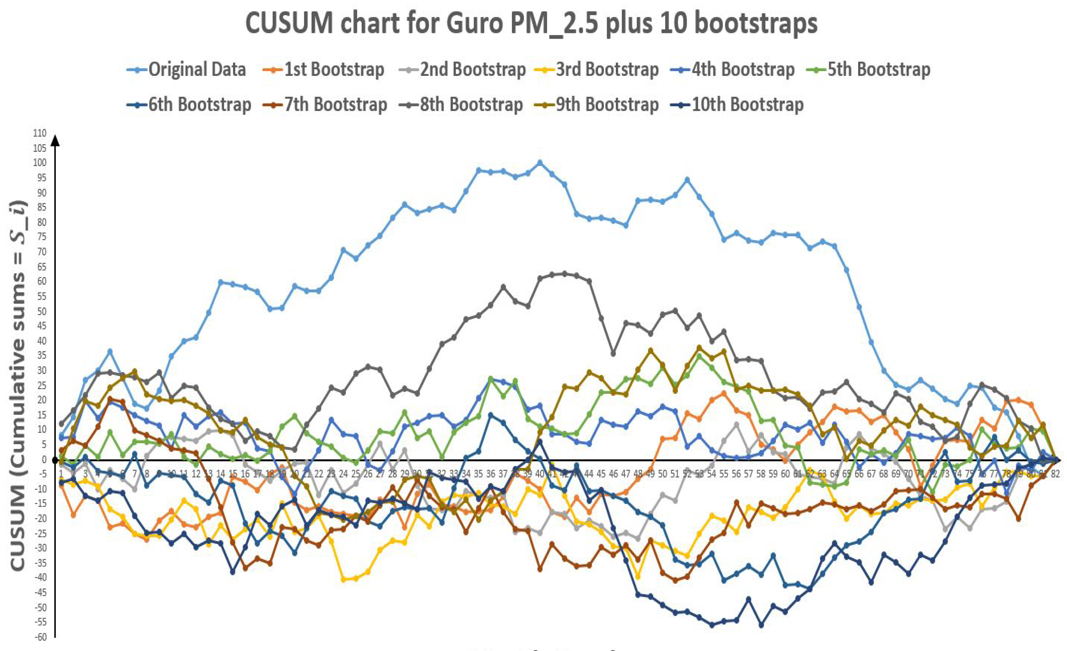
The idea behind bootstrapping is that the bootstrap samples represent random reordering of the data that mimic the behavior of the CUSUM if no change has occurred. By performing a large number of bootstrap samples, it can be estimated that how much S d i f f would vary if no change took place. It would be compared with the S d i f f value calculated from the data in its original order to determine if this value is consistent with what has been expected if no change occurred. If bootstrap CUSUM charts tend to stay closer to zero than the CUSUM of the data in its original order, this leads one to suspect that a change must have occurred. A bootstrap analysis consists of performing a large number of bootstraps and counting the number of bootstraps for which S 0 d i f f is less than S d i f f . Let N be the number of bootstrap samples performed and let X be the number of bootstraps for which S 0 d i f f < S d i f f . Then the confidence level that a change occurred as a percentage is calculated as follows:
Confidence Level = 100 X N percentage
This is strong evidence that a change did in fact occur. Ideally, rather than bootstrapping, one would like to determine the distribution of S 0 d i f f based on all possible reordering of the data. However, this is generally not feasible. A better estimate can be obtained by increasing the number of bootstrap samples. Bootstrapping results in a distribution free approach with only a single assumption, that of an independent error structure. Both control charting and change-point analysis are based on the mean-shift model. Let X 1 , X 2 , X 3 , represent the data in time order. The mean-shift model can be written as
X i = μ i + ϵ i
where μ i is the average at time i. Generally μ i = μ i 1 except for a small number of values of i called the change-points. ϵ i is the random error associated with the ith value. It is assumed that the ϵ i are independent with means of zero. Once a change has been detected, an estimate of when the change occurred can be made. One such estimator is the CUSUM estimator. Let m be such that:
S m = max i = 0 , 1 , 2 , , S i
S m is the point furthest from zero in the CUSUM chart. The point m estimates last point before the change occurred. The point m + 1 estimates the first point after the change. Once a change has been detected, the data can be broken into two segments, one each side of the change-point, 1 to m and m + 1 to 24, estimating the average of each segment, and then analyzing the two estimated averages.

4. Numerical Example

The formulated mathematical model has been used for the numerical verification and the validity of the model has also been checked. That is why real-time data of particulate matter hazards for four different sites of Seoul, South Korea has been utilized for this investigation.

4.1. Particulate Matter ( P M 2.5 ) and ( P M 10 ) Change Points for Four Different Sites

Two dissimilar cases need to be considered.

4.1.1. Case 1—When There Is No Hazard

In this case, there is no hazard and concentrations of particulate matter does not exceed the threshold value of the standards. Therefore, there will be no polluted day and random variable Y would always be y = 0 . Hence, due to zero hazard in the concentrations of particulate matter, this model has not been applied.

4.1.2. Case 2—When There Are Hazards

In this case, several polluted days for particulate matter ( P M 2.5 and P M 10 ) concentrations are considered as a Poisson process. A counting process is a Poisson counting process with the rate θ > 0 . Here, we report the results obtained by applying the method described in Section 3 to the particulate matter ( P M 2.5 and P M 10 ) concentrations for four different sites (Guro, Nowon, Songpa, and Yongsan) in Seoul, South Korea. We used the daily data observed from January 2004 to December 2013 to compute the change point of both pollutants.
f ( y ; θ ) = ( P r ( Y = y | θ ) ) = P o i s s o n ( y , θ ) = e θ θ y y ! f o r y 1 , 2 , . , n
Poisson distribution is the number of events occurring in a given time period. So in this case, occurrence of the number of polluted days in a month is taken as Poisson distribution. The rate of polluted days for both P M 2.5 and P M 10 are given in Table 7 and Table 8 respectively.
The change point for this Poisson process has to be detected to know whether a change has occurred, the most likely month in which change has occurred, and if the rate of polluted days has increased or decreased after the change point. It has been assumed that the number of polluted days for (particulate matter) P M 2.5 and P M 10 concentrations follows a Poisson distribution with a mean rate θ until the month k. After the month k, the polluted days are distributed according to the Poisson distribution with a mean rate λ . It can be represented as:
y i P o i s s o n ( θ ) for i = 1 , 2 , . , k
y i P o i s s o n ( λ ) for i = k + 1 , k + 2 , , n
Hence,
f ( y ; θ ) = P r ( Y = y i | θ ) for i = 1 , 2 , . , k
f ( y ; λ ) = P r ( Y = y i | λ ) for i = k + 1 , k + 2 , , n
If we model Y = y i as Poisson with mean rate θ then joint pdf of our sample data will be as below:
P r ( Y = y i | θ ) = i = 1 n p r ( y i | θ ) = i = 1 n e θ θ y i y ! = c ( y 1 , y 2 , y n ) e n θ θ y i i 0 , 1 , 2 , , n
This means that whatever our conjugate class of densities is, it will have to include terms like e C 2 θ θ C 1 for constants C 1 and C 2 . The simplest class of such densities, which include these terms and corresponding probability distributions, are known as family of Gamma distributions. Therefore, prior distribution P r ( θ ) and posterior distribution P r ( Y = θ | y 1 , y 2 , y n ) will follow a Gamma distribution, but likelihood or sampling model P r ( y 1 , y 2 , y n | θ ) follow a Poisson distribution.
Therefore, the prior distributions of θ and λ , uncertain positive quantities θ and λ has G a m m a ( a 1 , b 1 ) and G a m m a ( a 2 , b 2 ) distributions respectively, where a 1 is shape parameter and b 1 is rate parameter for θ while a 2 is shape parameter and b 2 is rate parameter for λ
P r ( θ ) = G a m m a ( θ , a 1 , b 1 ) = b 1 a 1 e b 1 θ θ a 1 1 Γ ( a 1 )
P r ( λ ) = G a m m a ( λ , a 2 , b 2 ) = b 2 a 2 e b 2 λ λ a 2 1 Γ ( a 2 )
Gamma distribution is also conjugate prior of the rate (inverse scale) parameter of the Gamma distribution itself. That is why the rate parameter b 1 and b 2 will also follow a Gamma distribution with different shape and rate parameters as given below:
b 1 G a m m a ( c 1 , d 1 ) where c 1 = shape parameter d 1 = rate parameter
b 2 G a m m a ( c 2 , d 2 ) where c 2 = shape parameter d 2 = rate parameter
By applying Bayes theorem, posterior distributions for rate parameters θ , λ , b 1 and b 2 will be determined in the following way. Likelihood and prior distributions of θ
P r ( y 1 , y 2 , y 3 , . , y n | θ ) P o i s s o n ( θ )
P r ( θ ) = G a m m a ( θ , a 1 , b 1 )
P r ( θ | y 1 , y 2 , y 3 , . , y n ) = P r ( y 1 , y 2 , y 3 , . , y n | θ ) P r ( θ ) P r ( y 1 , y 2 , y 3 , . , y n ) = ( e b 1 θ θ a 1 1 ) × ( e n θ θ y i ) × c ( y 1 , y 2 , y 3 , . , y n ) = ( e ( b 1 + n ) θ θ a 1 + y i 1 ) × c ( y 1 , y 2 , y 3 , . , y n , a 1 , b 1 ) ( θ | y 1 , y 2 , y 3 , . , y n ) G a m m a ( a 1 + i = 1 n y i , b 1 + n )
This is evidently a Gamma distribution. Hence, the conjugacy of Gamma family for the Poisson sampling model or likelihood is confirmed. Hence, it is concluded from the above that if:
θ G a m m a ( a 1 , b 1 )
P r ( y 1 , y 2 , y 3 , . , y n | θ ) P o i s s o n ( θ )
Then:
( θ | y 1 , y 2 , y 3 , . , y n ) G a m m a ( a 1 + i = 1 n y i , b 1 + n )
Similarly, the posterior distributions of all parameters θ , λ , b 1 and b 2 can be determined as given below:
( θ | y , λ , b 1 , b 2 , k ) G a m m a ( a 1 + i = 1 k y i , k + b 1 )
( λ | y , θ , b 1 , b 2 , k ) G a m m a ( a 2 + i = k + 1 n y i , k + b 2 )
( b 1 | y , θ , λ , b 2 , k ) G a m m a ( a 1 + c 1 , θ + d 1 )
( b 2 | y , θ , λ , b 1 , k ) G a m m a ( a 2 + c 2 , λ + d 2 )
As Gamma is a two-parameter family of continuous probability distribution. As a result, the function:
L ( θ | Y ) = f θ ( Y ) = f ( Y | θ )
The likelihood ratio test statistic is:
f ( k | Y , θ , λ ) = L ( Y ; k , θ , λ ) j = 1 n L ( Y ; j , θ , λ )
The likelihood is determined as given by:
L ( Y ; k , θ , λ ) = e x p ( k ( λ θ ) ) ( θ / λ ) i = 1 k y i
For Bayesian approach, MATLAB has been used for change point detection of particulate matter ( P M 2.5 and P M 10 ) data during the study period (2004–2013) for four different sites (Guro, Nowon, Songpa and Yongsan) in Seoul, South Korea. 10 replications of each simulation are made with 1100 observations in each replication. First 100 observations are discarded as a burn-in period. Replication Mean V i of remaining 1000 observations has been taken for each replication as shown in Table 9 and Table 10. Then mean ( V ) of replication mean has been taken to get the converged values of parameters.
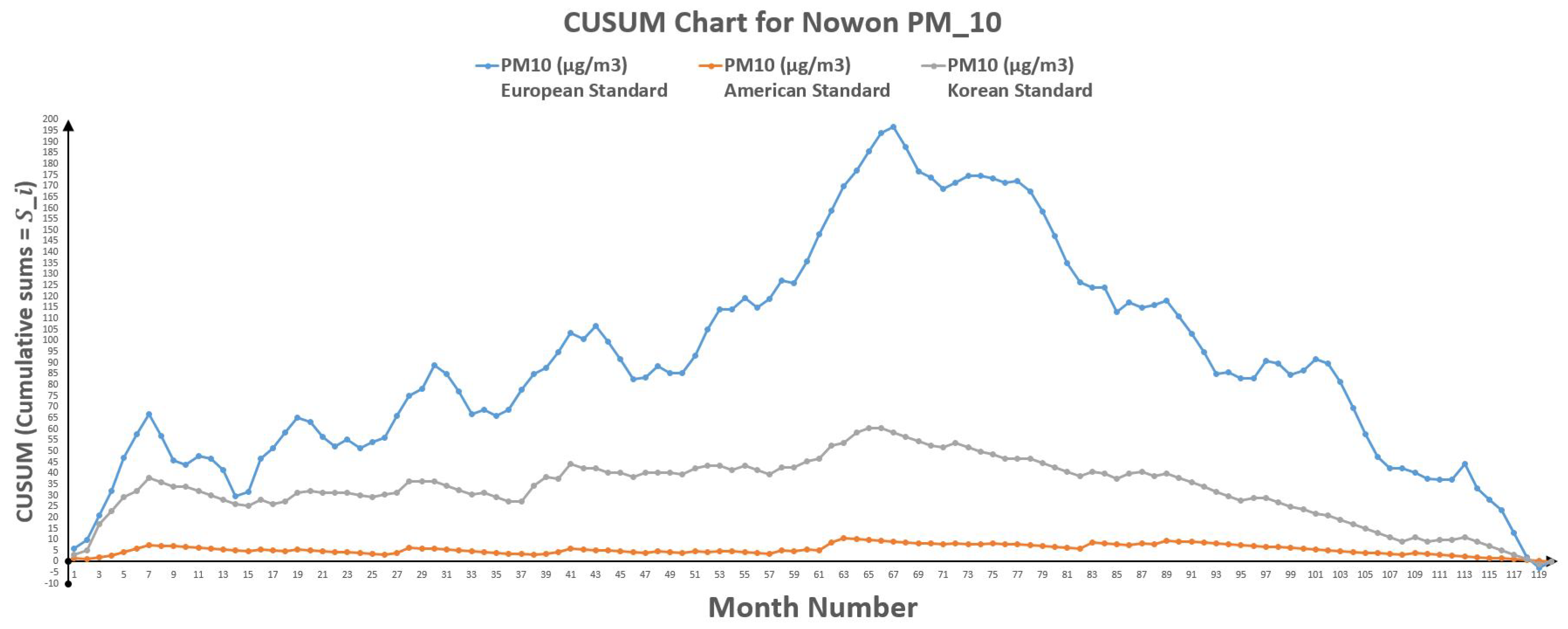
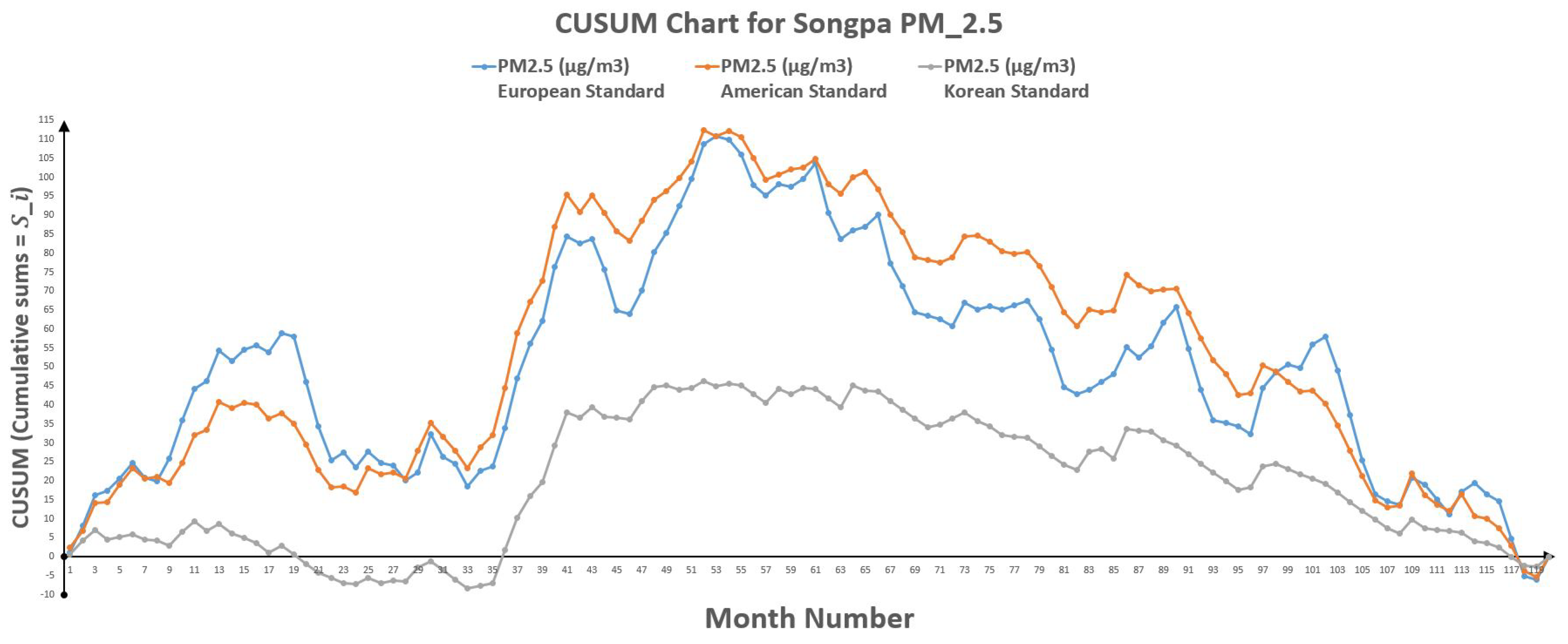
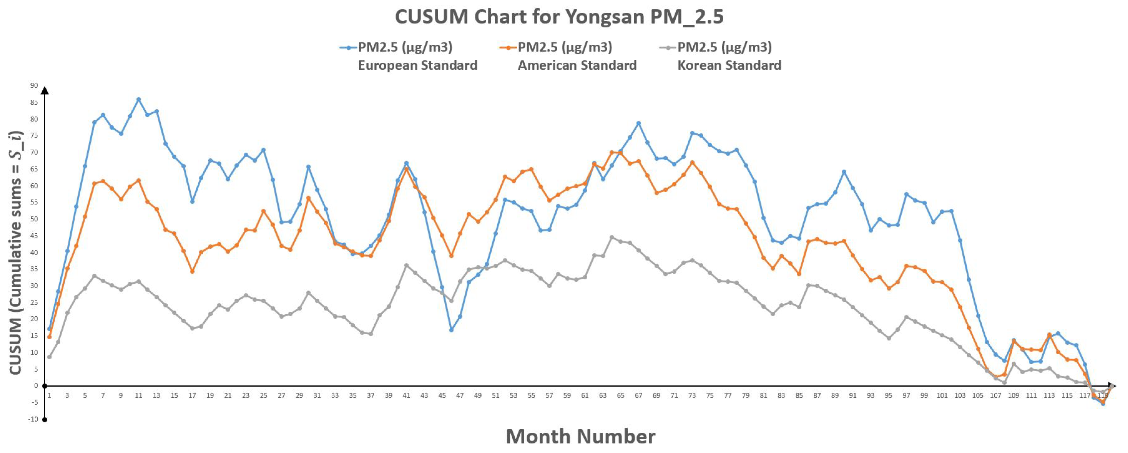
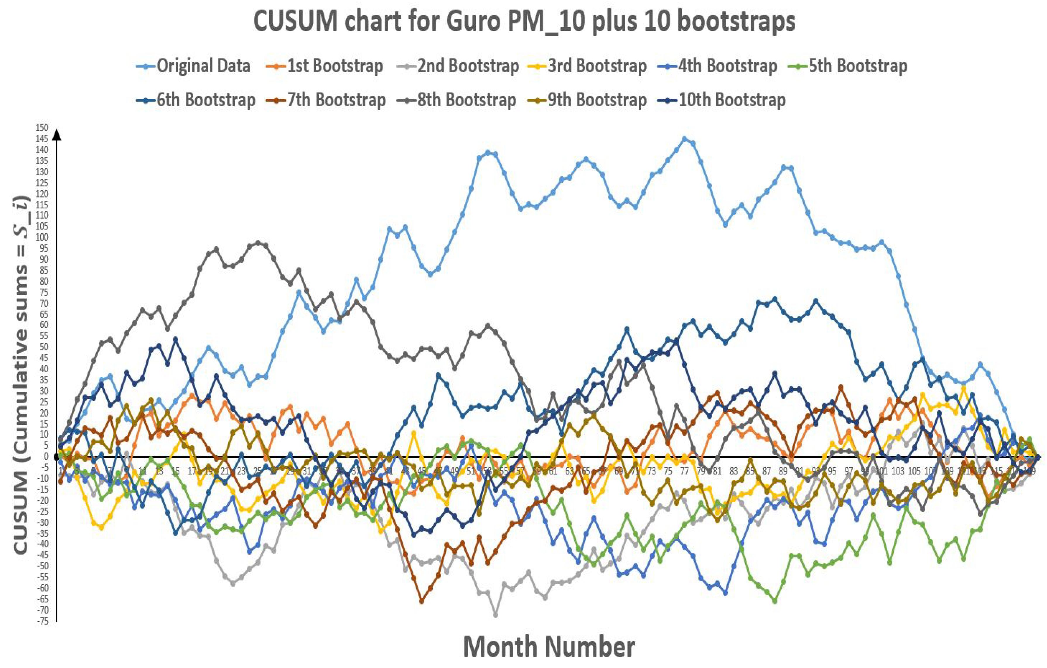
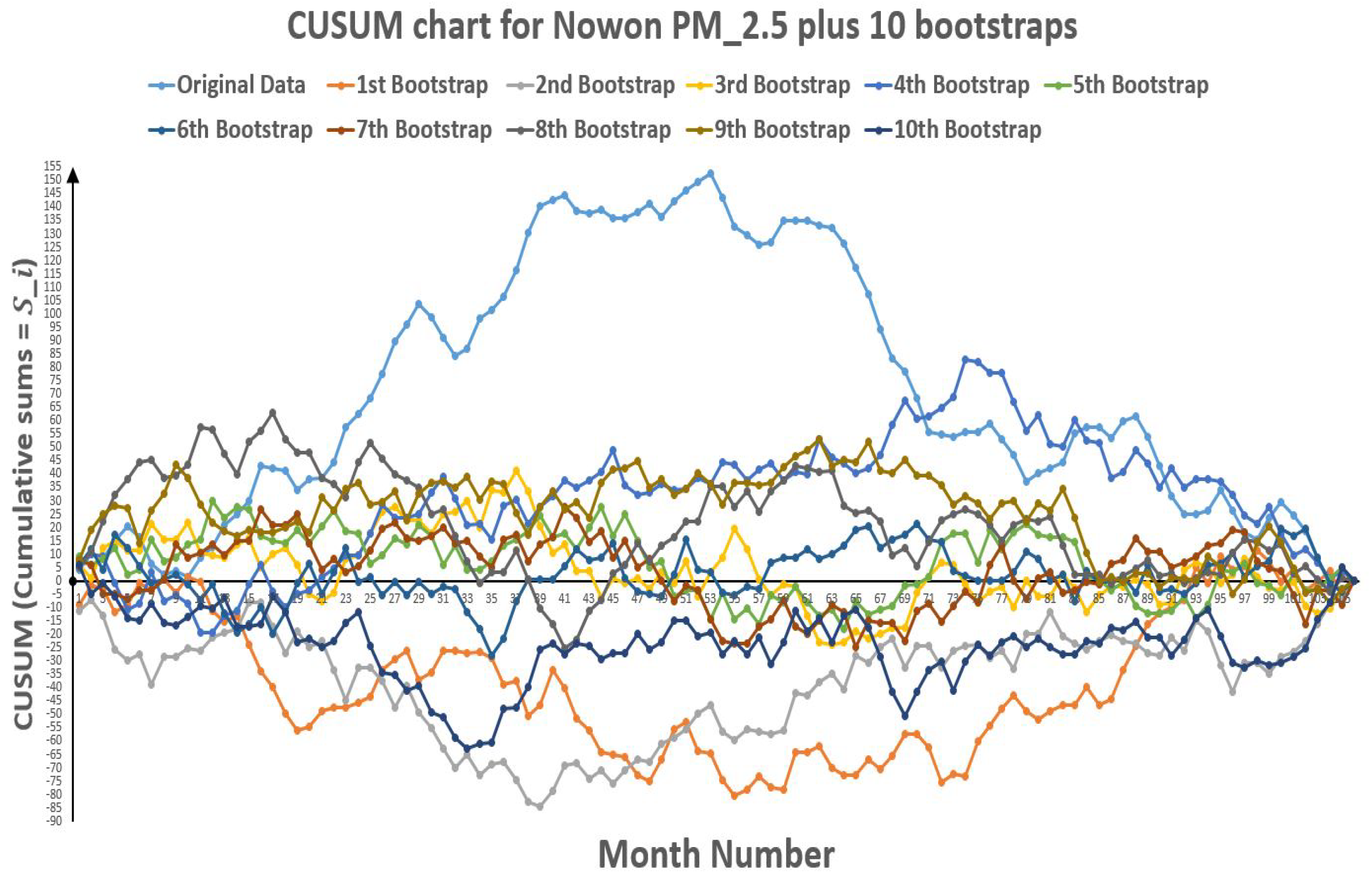
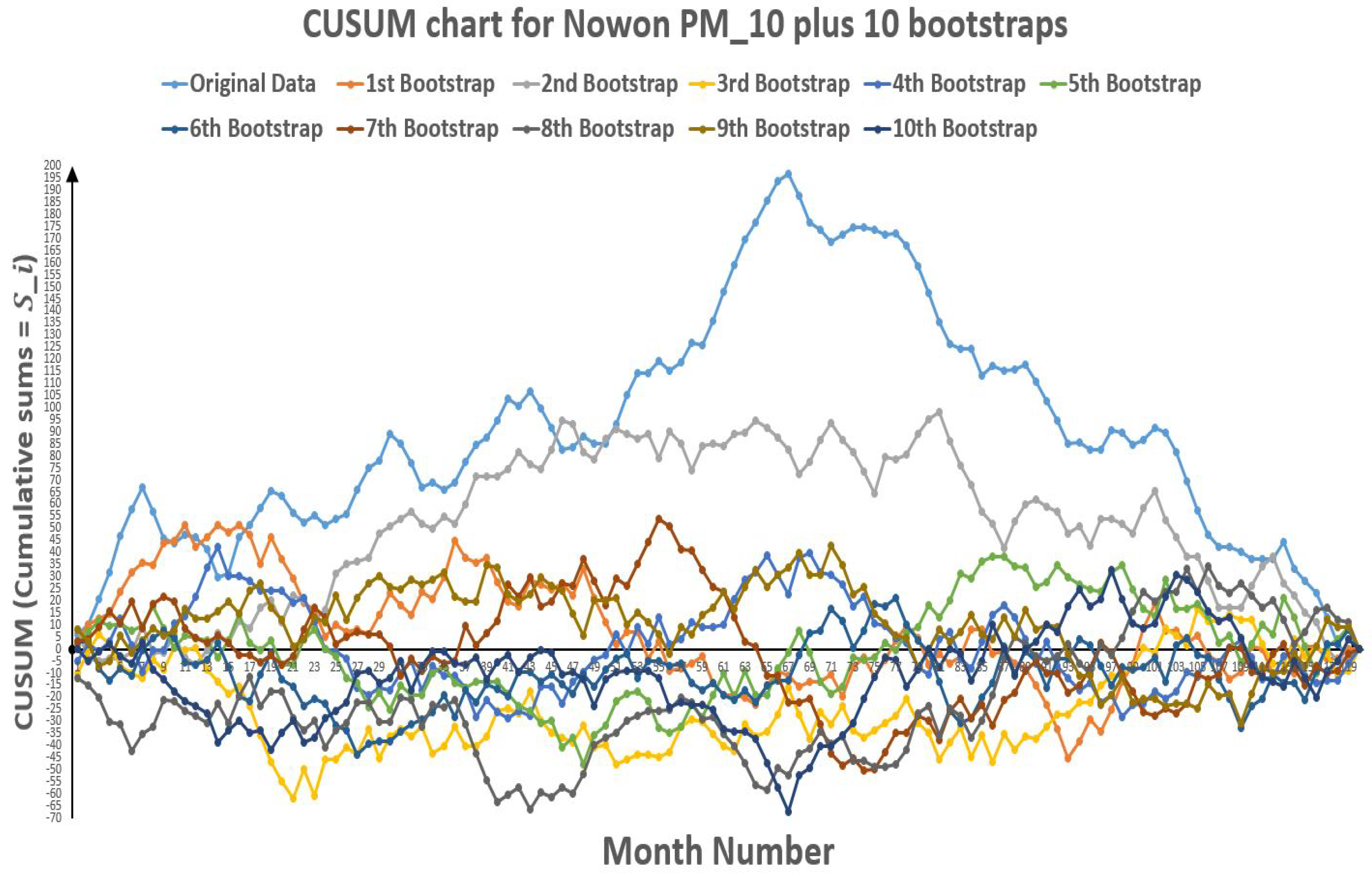
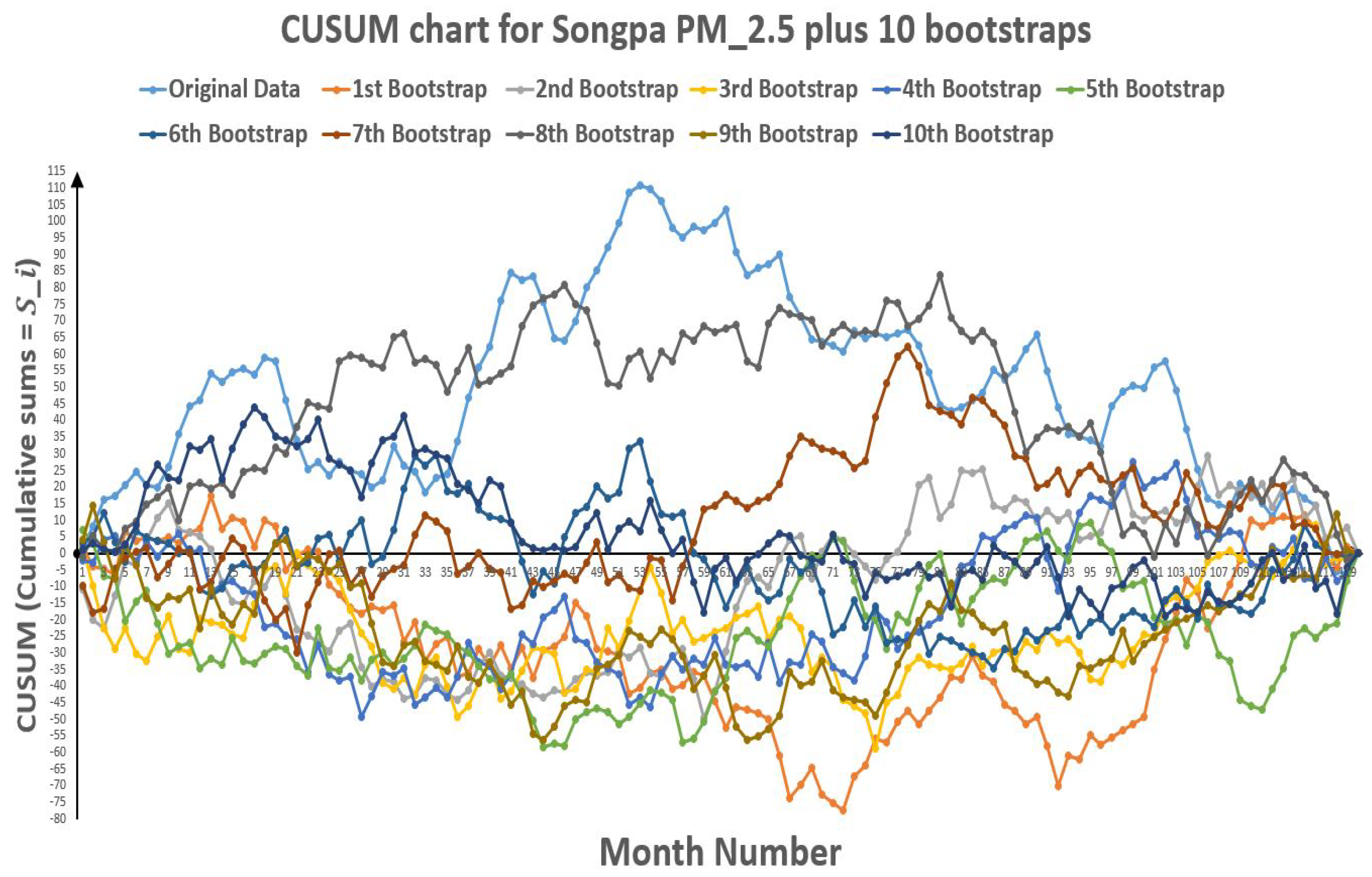
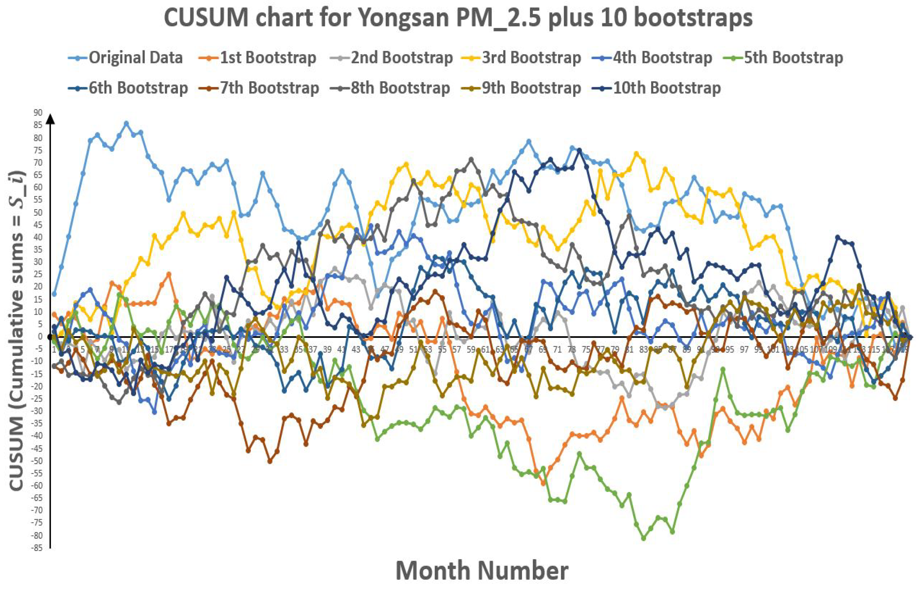
Moreover, the CUSUM charts of polluted days as per European, American and Korean standards are shown in Figure 2, Figure 3, Figure 4, Figure 5, Figure 6, Figure 7, Figure 8 and Figure 9 for four different sites Guro, Nowon, Songpa and Yongsan in Seoul, South Korea.
However, the bootstraps analysis of European standards has been shown in Figure 10, Figure 11, Figure 12, Figure 13, Figure 14, Figure 15, Figure 16 and Figure 17 as given below.
The change point k is discrete uniform over ( 1 , 2 , 3 120 ) as there are 120 months in 10 years. Please note that θ , λ and k are all independent of each other.

5. Numerical Results

Two dissimilar approaches have been used to attain the results. First one is Bayesian approach, which is based on probability distributions. It can be applicable to any kind of data distribution. For this, firstly data distributions are defined and then proposed method is applied to acquire the results. This approach is better to apply for random data structures and time series. While the second method is based on CUSUM charts, this technique is directly applicable on the raw data, which is good for deterministic data structures. Summarized forms of particulate matter ( P M 2.5 and P M 10 ) change point (k), the rate before change point ( θ ) and the rate after change point ( λ ) during the study period (2004–2013) for four different sites (Guro, Nowon, Songpa and Yongsan) in Seoul, South Korea are given in Table 11, Table 12, Table 13 and Table 14. The results have been computed by following the European, American, and Korean Standards as discussed in Table 4.

5.1. P M 2.5 Change Point (k) through Bayesian Approach

In Table 11, the results obtained through Bayesian approach have been described, where ( k ) is the predicted change point varies for different areas and different air quality standards. The results indicate the reduction of polluted days after change point ( k ) for P M 2.5 . While ( θ ) represents the per month rate of polluted days before change point, ( k ) and ( λ ) be the rate of per month polluted days after change point ( k ) .

5.2. P M 2.5 Last Point before Change (k) and First Point after Change ( k + 1 ) through CUSUM Approach

Table 12 represents the results obtained for P M 2.5 through CUSUM approach, where ( k ) is the last point before change and ( k + 1 ) be the first point after change point. So, the change point leis somewhere between ( k ) and ( k + 1 ) . This method also shows the reduction of polluted days after change point as ( θ ) represents the per month rate of polluted days before change point and ( λ ) be the rate of per month polluted days after change point.

5.3. P M 10 Change Point (k) through Bayesian Approach

Table 13 explains the results obtained for P M 10 through Bayesian approach. Hence, the expected change point is ( k ) that differs for different areas and various air quality standards. These results show the reduction of polluted days after change point ( k ) for P M 10 . While ( θ ) is the per month rate of polluted days before change point ( k ) and ( λ ) represents the rate of per month polluted days after change point ( k ) .

5.4. P M 10 Last Point before Change (k) and First Point after Change ( k + 1 ) through CUSUM Approach

The results obtained for P M 10 through CUSUM approach have been described in Table 14, where the last point before change is ( k ) and the first point after change point is ( k + 1 ) . Therefore, the change point leis anywhere between ( k ) and ( k + 1 ) . This method also depicts the reduction of polluted days after change point. ( θ ) represents the per month rate of polluted days before change point and ( λ ) be the rate of per month polluted days after change point.

6. Disussion

As the results of two different approaches have been described in the previous section.
  • Bayesian approach is based on probability distributions, which can be applicable on any kind of data distribution. In this case, firstly data distributions are defined and then proposed method is applied to acquire the results. This approach is better to apply for random data structures and time series.
  • CUSUM Approach is directly applied on the raw data, which is good for deterministic data structures.

6.1. Guro (Seoul, South Korea)

Guro is located in the southwestern part of Seoul, and has an important position as a transport link which includes railroads and land routes. The largest digital industrial complex in Korea is also positioned in Guro, centering on research and development activities as well as advanced information and knowledge industries. That is why, the policies of the Ministry of Environment in South Korea have influenced the concentrations of particulate matters ( P M 2.5 and P M 10 ) in Guro and rate of polluted days has reduced in any of the cases.

6.1.1. Bayesian Approach

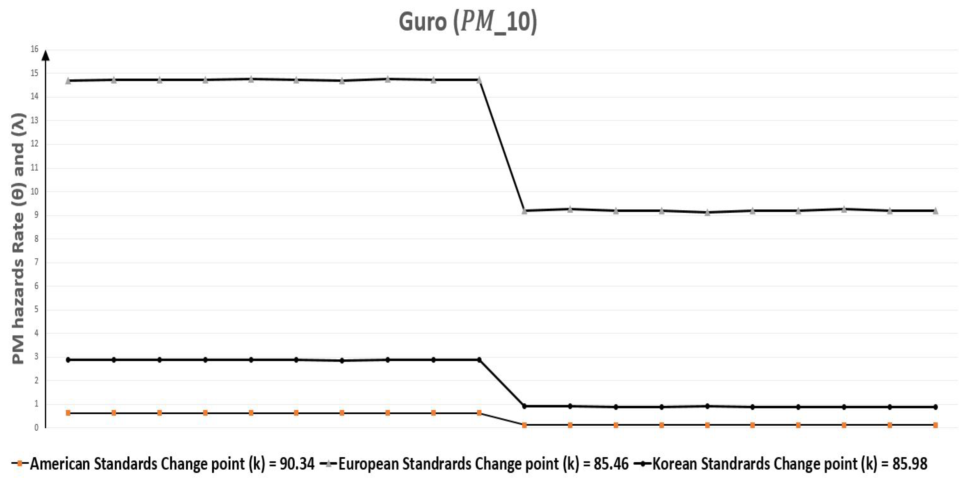
Bayesian method is better to apply for random time series data. If we look in case of Guro, Table 11 indicates that for P M 2.5 change-point (k) of polluted days were 43.18, 33.62, and 38.26 according to European, American, and Korean standards respectively. Therefore, a change occurred in the rate of polluted days, but it varied according to standards. At the minimum, the rate of polluted days ( θ = 15.99) was reduced 30.14% and the maximum reduction ( θ = 3.56) to ( λ = 1.63) was 54.21% in the case of Korean standards. Similarly, Table 13 refers to the reduction of polluted days ( θ ) to ( λ ) for P M 10 after change point (k) which were 85.46, 90.34, and 85.98 according to European, American, and Korean standards, respectively. Moreover, the decrease in the rate of polluted days ( θ = 14.73) to ( λ = 9.20) was at least 37.54% for European standards, but it was 80.95% in the case of American standards. Figure 18 and Figure 19 graphically represent the replications of monthly polluted days before and after the change point which are discussed in Table 9 and Table 10.

6.1.2. CUSUM Approach

CUSUM Approach also indicates a reduction in hazards rate from ( θ ) to ( λ ) after change. As for Guro, Table 12 also represents the change of P M 2.5 polluted days through CUSUM approach, which shows that change point occurred between point 40 (k) and 41 ( k + 1 ) for European standards, between point 36 (k) and 37 ( k + 1 ) for American standards and it lies in-between point 35 (k) and 36 ( k + 1 ) for Korean standards. While Table 14 indicates the change of P M 10 polluted days through CUSUM approach with an indication of change point lies between point 77 (k) and 78 ( k + 1 ) for European standards, point 89 (k) and 90 ( k + 1 ) for American standards and point 64 (k) and 65 ( k + 1 ) for Korean standards.

6.2. Nowon (Seoul, South Korea)

Nowon is located in the northeastern part of the city, and has the highest population density in Seoul with 619,509 persons living in 35.44 km 2 , which is surrounded by mountains and forests on the northeast. The policies of the Ministry of Environment in Nowon have improved the rate of polluted days for P M 2.5 and P M 10 hazards from θ to λ . Improvement in the reduction of polluted days varies case to case.

6.2.1. Bayesian Approach

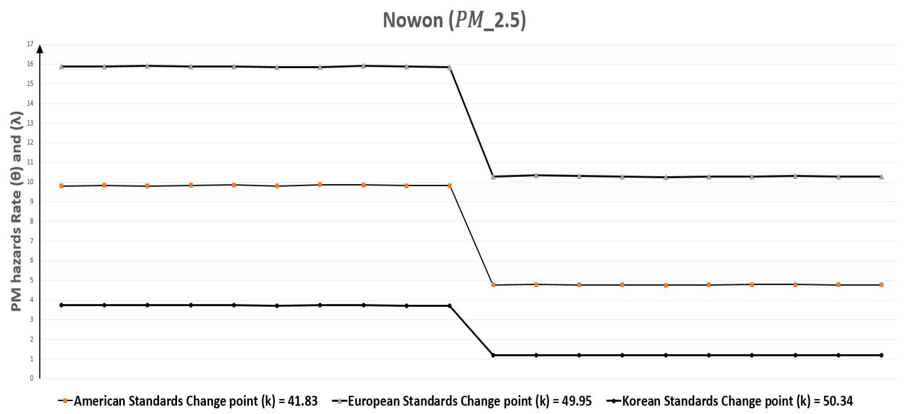
Correspondingly, in case of Nowon, Table 11 depicts that change point (k) of polluted days for P M 2.5 were 49.95, 41.83, and 50.34 according to European, American, and Korean standards respectively. Particularly for this case, the change point was the same according to European and Korean standards, but varied for American standards. The rate of polluted days ( θ = 15.88) for European standards showed a minimum decrease of 35.14% after the change point and approached ( λ = 10.30), but the maximum decrease was for Korean standards which was 67.65% with ( θ = 3.74) and ( λ = 1.21). In the same manner, when we study Table 13, it elaborates that for P M 10 , again there was a reduction in the rate of polluted days after change point (k) of 67.12, 73.80, and 65.68 to European, American, and Korean standards, respectively. That is comparable in cases of European and Korean standards, but a bit different for American standards. In addition, the reduction in the rate of polluted days for the European standard was at least 44.01% from ( θ = 14.93) to ( λ = 8.36), while the maximum reduction was ( θ = 0.62) to ( λ = 0.11) 82.25% for American standards. Figure 20 and Figure 21 graphically represent the replications of monthly polluted days before and after the change point which are given in Table 9 and Table 10.

6.2.2. CUSUM Approach

Moreover, CUSUM Approach also validates the reduction of PM hazards. In case of Nowon, Table 12 represents the change of P M 2.5 polluted days through CUSUM approach, which shows that change point occurred between point 53 (k) and 54 ( k + 1 ) for European standards, between point 41 (k) and 42 ( k + 1 ) for American standards and it lies in-between point 50 (k) and 51 ( k + 1 ) for Korean standards. While Table 14 indicates the change of P M 10 polluted days through CUSUM approach with an indication of change point lies between point 67 (k) and 68 ( k + 1 ) for European standards, point 63 (k) and 64 ( k + 1 ) for American standards and point 66 (k) and 67 ( k + 1 ) for Korean standards.

6.3. Songpa (Seoul, South Korea)

Songpa is located at the southeastern part of Seoul, and has largest population, with 647,000 residents. As per Ministry of Environment policies in Songpa, there is a smaller reduction for the rate of polluted days ( θ ) to ( λ ) as compared to Guro and Nowon, but still there is a significant reduction in PM hazards.

6.3.1. Bayesian Approach

Now for Songpa, we can check from Table 11 that change point (k) of polluted days for P M 2.5 were 53.85, 53.32, and 56.44 for European, American, and Korean standards respectively, which were all similar. The reduction in rate of polluted days was at least 24.50% for European Standards ( θ = 14.90) to ( λ = 11.25) while it was highest for Korean standards at 47.77% with ( θ = 3.14) and ( λ = 1.64). Correspondingly, we can also inspect the improvement in the rate of polluted days from ( θ ) to ( λ ) for P M 10 after change point (k) in Table 13. Change point (k) for the rate of polluted days due to P M 10 concentration were 53.50, 88.16, and 52.75 according to European, American and Korean standards respectively, which was the same for European and Korean standards. The slightest improvement 41.17% has been in the case of European standards and ( θ = 16.08) is converted to ( λ = 9.46). On the other hand, if we look at American standards, the rate of polluted days ( θ = 0.56) was already low which further decreased 87.5% to ( λ = 0.07). Hence, this area is almost a meeting of the P M 10 concentration requirements for American standards but not for other standards. Figure 22 and Figure 23 graphically represent the replications of monthly polluted days before and after the change point which are given in Table 9 and Table 10.

6.3.2. CUSUM Approach

As per CUSUM Approach, there is a decrease in PM hazards. Table 12 also represents the change of P M 2.5 polluted days through CUSUM approach, which shows that change point occurred between point 53 (k) and 54 ( k + 1 ) for European standards, between point 52 (k) and 53 ( k + 1 ) for American standards and it lies in-between point 52 (k) and 53 ( k + 1 ) for Korean standards. While Table 14 indicates the change of P M 10 polluted days through CUSUM approach with an indication of change point lies between point 53 (k) and 54 ( k + 1 ) for European standards, point 53 (k) and 54 ( k + 1 ) for American standards and point 52 (k) and 53 ( k + 1 ) for Korean standards.

6.4. Yongsan (Seoul, South Korea)

Yongsan is a place in the center of Seoul in which almost 250,000 people reside. Prominent locations in Yongsan includes Yongsan station, electronic market and Itaewon commercial area with heavy traffic and transportation. Consequently, the policies of the Ministry of Environment in Yongsan has affected the particulate matter ( P M 2.5 and P M 10 ) concentrations more than all the previous three locations (Guro, Nowon and Songpa). There is a remarkable decrease in rate of polluted days from ( θ ) to ( λ ).

6.4.1. Bayesian Approach

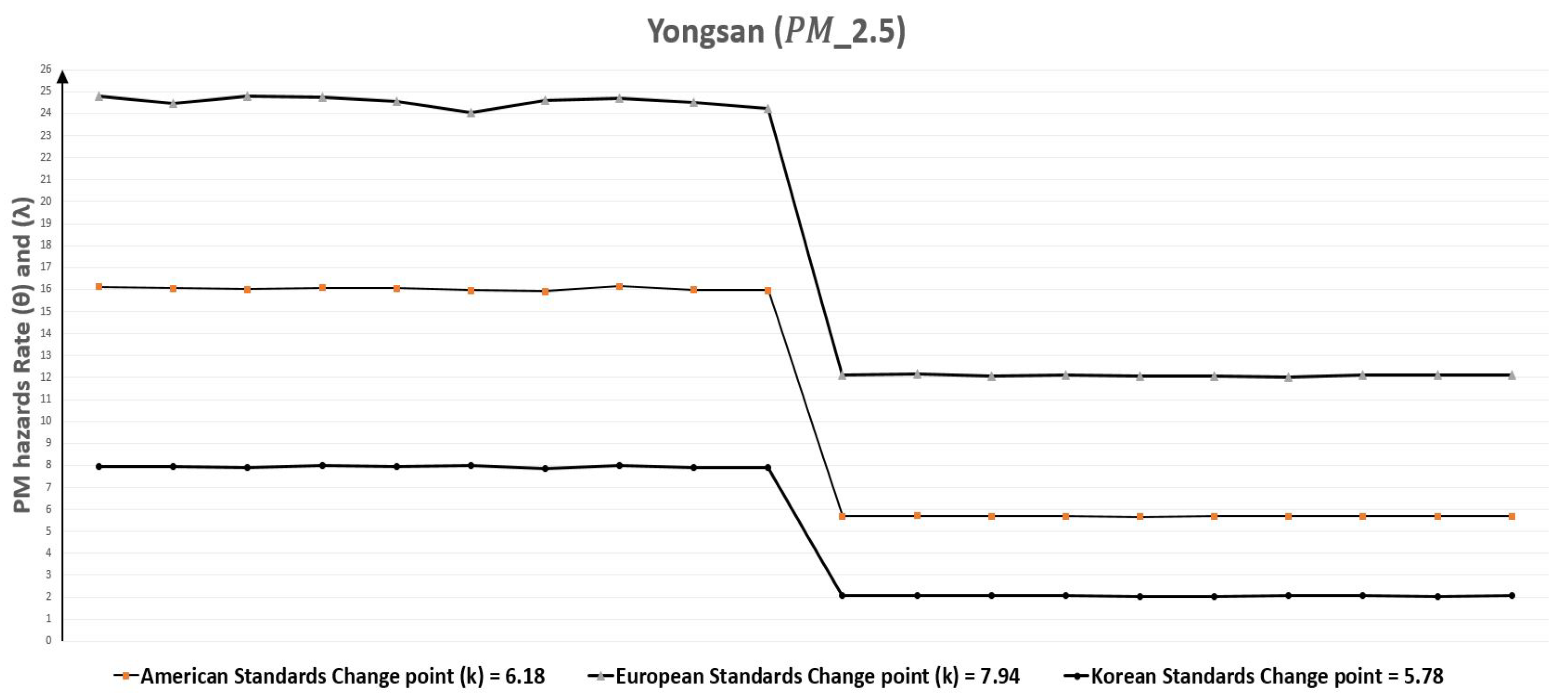
Similarly, in the case of Yongsan, Table 11 and Table 13 tell us that the rate of polluted days ( θ ) for particulate matters ( P M 2.5 and P M 10 ) was the highest in Seoul. The change occurred for P M 2.5 with the change point (k) 7.94, 6.18, and 5.78 with respect to European, American and Korean standards respectively, which was comparable for all the three standards. There was minimally a 50.71% fall in the rate of polluted days ( θ = 24.55) to ( λ = 12.10) for European standards, but the reduction in rate of polluted days was a maximum of 74.18% in the case of Korean standards. On the same note, Table 13 indicates that the change in the rate of polluted days has also occurred for P M 10 concentrations. The change point (k) for it were 89.74, 91.36, and 68.06 for European, American and Korean standards, respectively. Furthermore, at least 42.10% rate of polluted days ( θ = 14.56) was reduced to ( λ = 8.43) for European standards but its maximum decrease was 93.93% for American standards ( θ = 0.66) to ( λ = 0.04), although, it is already approaching the requirements of this standard. Figure 24 and Figure 25 graphically represent the replications of monthly polluted days before and after the change point which are given in Table 9 and Table 10.

6.4.2. CUSUM Approach

CUSUM Approach is directly applied on the raw data, which should be better for deterministic data structures. It also shows a reduction in PM hazards. In case of Yongsan, Table 12 also represents the change of P M 2.5 polluted days through CUSUM approach, which shows that change point occurred between point 11 (k) and 12 ( k + 1 ) for European standards, between point 64 (k) and 65 ( k + 1 ) for American standards and it lies in-between point 64 (k) and 65 ( k + 1 ) for Korean standards. While Table 14 indicates the change of P M 10 polluted days through CUSUM approach with an indication of change point lies between point 77 (k) and 78 ( k + 1 ) for European standards, point 89 (k) and 90 ( k + 1 ) for American standards and point 64 (k) and 65 ( k + 1 ) for Korean standards.

6.5. Strengths

  • This approach is very precise, well defined, user friendly and easily understandable for applications on probability distributions, time series and random data.
  • The above mentioned model is an appropriate approach for detection of change points in random data structures.
  • Good technique for evaluation of process control programs by comparing the parameters before and after change point.

6.6. Limitations

  • Detection of only single change point is given in this model.
  • Further extension is required by making a model for a multiple number of change points for locating changed segments.

6.7. Managerial Insights

  • This model presents a suitable technique to analyze the air quality and pollutant hazards in the air.
  • By detecting change points in particulate matter ( P M 2.5 and P M 10 ) concentrations and analyzing the occurrences of polluted days before and after a change point, environmental protection agencies can understand the role of their legislation efforts, and whether these change points are favorable or not for the environment.
  • A comparison of particulate matter hazards before and after a change point evaluates a pollution control program adopted by environmental protection agencies to make a decision. If these policies need further revision or not for the reduction of death rates and burden of diseases due airborne particulate matter concentrations in the air.
  • This study of pollutant hazards also defines the current levels of subjected air pollutant in the air which is helpful to make new pollution control policies for further improvements.
  • This research also brings an intuition to define new goals if previously defined goals have been achieved and also provides a vision if the environmental standards need to be revised, or not to overcome environmental challenges.

7. Conclusions

The main focus of this research work was to elucidate an appropriate change point detection model for occurrences of pollutant hazards due to higher concentrations of particulate matter ( P M 2.5 and P M 10 ) in different locations. The rate of pollutant hazards before and after a change point was also estimated comprehensively to investigate the effectiveness of policies applied by the Ministry of Environment. To verify the model, four major locations (Guro, Nowon, Songpa, and Yongsan) in Seoul, South Korea were selected as study areas due to their different characteristics, such as climate zones, environment, populations and population densities. Three different environmental standards (European, American and Korean) were chosen as threshold values. Then, the model was applied to real time data sets in all cases and conclusions were drawn. The rate before and after the change point of particulate matter concentrations indicated a reduction in polluted days over a 10-year period. The overall results of our study confirm the effective role of legislation efforts used consistently to improve the air quality through the years but pollutant hazards still exist. Hence, further improvements are required to meet set standards to nullify hazards. This study can be further extended by making a multi-parameter change point model for a multiple number of change points considering the fact that different data structures follow different probability distributions.

Author Contributions

Conceptualization, Muhammad Rizwan Khan (M.R.K.) and Biswajit Sarkar (B.S.); methodology, M.R.K.; software, M.R.K.; validation, M.R.K. and B.S.; formal analysis, M.R.K.; investigation, M.R.K.; resources, M.R.K. and B.S.; data curation, M.R.K. and B.S.; writing—original draft preparation, M.R.K.; writing—review and editing, B.S.; visualization, M.R.K. and B.S.; supervision, B.S.; project administration, M.R.K. and B.S.; funding acquisition, B.S.

Funding

This research received no external funding.

Conflicts of Interest

The authors declare no conflict of interest.

References

  1. Héroux, M.E.; Anderson, H.R.; Atkinson, R.; Brunekreef, B.; Cohen, A.; Forastiere, F.; Hurley, F.; Katsouyanni, K.; Krewski, D.; Krzyzanowski, M.; et al. Quantifying the health impacts of ambient air pollutants: recommendations of a WHO/Europe project. Int. J. Public Health 2015, 60, 619–627. [Google Scholar] [CrossRef] [PubMed] [Green Version]
  2. Pope, C.A.; Burnett, R.T.; Thurston, G.D.; Thun, M.J.; Calle, E.E.; Krewski, D.; Godleski, J.J. Cardiovascular mortality and long-term exposure to particulate air pollution: Epidemiological evidence of general pathophysiological pathways of disease. Circulation 2004, 109, 71–77. [Google Scholar] [CrossRef] [PubMed]
  3. Gyarmati-Szabó, J.; Bogachev, L.V.; Chen, H. Modelling threshold exceedances of air pollution concentrations via non-homogeneous Poisson process with multiple change-points. Atmos. Environ. 2011, 45, 5493–5503. [Google Scholar] [CrossRef] [Green Version]
  4. Pirani, M.; Best, N.; Blangiardo, M.; Liverani, S.; Atkinson, R.W.; Fuller, G.W. Analysing the health effects of simultaneous exposure to physical and chemical properties of airborne particles. Environ. Int. 2015, 79, 56–64. [Google Scholar] [CrossRef] [PubMed] [Green Version]
  5. Welty, L.J.; Peng, R.; Zeger, S.; Dominici, F. Bayesian distributed lag models: Estimating effects of particulate matter air pollution on daily mortality. Biometrics 2009, 65, 282–291. [Google Scholar] [CrossRef]
  6. Qin, S.; Liu, F.; Wang, J.; Sun, B. Analysis and forecasting of the particulate matter (PM) concentration levels over four major cities of China using hybrid models. Atmos. Environ. 2014, 98, 665–675. [Google Scholar] [CrossRef]
  7. Keshavarz, H.; Scott, C.; Nguyen, X. Optimal change point detection in Gaussian processes. J. Stat. Plan. Inference 2018, 193, 151–178. [Google Scholar] [CrossRef] [Green Version]
  8. Kucharczyk, D.; Wyłomańska, A.; Sikora, G. Variance change point detection for fractional Brownian motion based on the likelihood ratio test. Phys. Stat. Mech. Its Appl. 2018, 490, 439–450. [Google Scholar] [CrossRef]
  9. Lu, G.; Zhou, Y.; Lu, C.; Li, X. A novel framework of change-point detection for machine monitoring. Mech. Syst. Signal Process. 2017, 83, 533–548. [Google Scholar] [CrossRef]
  10. Taleizadeh, A.A.; Samimi, H.; Sarkar, B.; Mohammadi, B. Stochastic machine breakdown and discrete delivery in an imperfect inventory-production system. J. Ind. Manag. Optim. 2017, 13, 1511–1535. [Google Scholar] [CrossRef] [Green Version]
  11. Liu, S.; Yamada, M.; Collier, N.; Sugiyama, M. Change-point detection in time-series data by relative density-ratio estimation. Neural Netw. 2013, 43, 72–83. [Google Scholar] [CrossRef] [Green Version]
  12. Hilgert, N.; Verdier, G.; Vila, J.P. Change detection for uncertain autoregressive dynamic models through nonparametric estimation. Stat. Methodol. 2016, 33, 96–113. [Google Scholar] [CrossRef] [Green Version]
  13. Górecki, T.; Horváth, L.; Kokoszka, P. Change point detection in heteroscedastic time series. Econom. Stat. 2018, 7, 63–88. [Google Scholar] [CrossRef] [Green Version]
  14. Bucchia, B.; Wendler, M. Change-point detection and bootstrap for Hilbert space valued random fields. J. Multivar. Anal. 2017, 155, 344–368. [Google Scholar] [CrossRef] [Green Version]
  15. Shin, D.; Guchhait, R.; Sarkar, B.; Mittal, M. Controllable lead time, service level constraint, and transportation discounts in a continuous review inventory model. RAIRO-Oper. Res. 2016, 50, 921–934. [Google Scholar] [CrossRef]
  16. Zhou, M.; Wang, H.J.; Tang, Y. Sequential change point detection in linear quantile regression models. Stat. Probab. Lett. 2015, 100, 98–103. [Google Scholar] [CrossRef]
  17. Lu, K.P.; Chang, S.T. Detecting change-points for shifts in mean and variance using fuzzy classification maximum likelihood change-point algorithms. J. Comput. Appl. Math. 2016, 308, 447–463. [Google Scholar] [CrossRef]
  18. Sarkar, B.; Saren, S. Partial trade-credit policy of retailer with exponentially deteriorating items. Int. J. Appl. Comput. Math. 2015, 1, 343–368. [Google Scholar] [CrossRef]
  19. Ruggieri, E.; Antonellis, M. An exact approach to Bayesian sequential change point detection. Comput. Stat. Data Anal. 2016, 97, 71–86. [Google Scholar] [CrossRef] [Green Version]
  20. Keshavarz, M.; Huang, B. Bayesian and Expectation Maximization methods for multivariate change point detection. Comput. Chem. Eng. 2014, 60, 339–353. [Google Scholar] [CrossRef]
  21. Kurt, B.; Yıldız, Ç.; Ceritli, T.Y.; Sankur, B.; Cemgil, A.T. A Bayesian change point model for detecting SIP-based DDoS attacks. Digit. Signal Process. 2018, 77, 48–62. [Google Scholar] [CrossRef]
  22. Wu, C.; Du, B.; Cui, X.; Zhang, L. A post-classification change detection method based on iterative slow feature analysis and Bayesian soft fusion. Remote. Sens. Environ. 2017, 199, 241–255. [Google Scholar] [CrossRef]
  23. Mariño, I.P.; Blyuss, O.; Ryan, A.; Gentry-Maharaj, A.; Timms, J.F.; Dawnay, A.; Kalsi, J.; Jacobs, I.; Menon, U.; Zaikin, A. Change-point of multiple biomarkers in women with ovarian cancer. Biomed. Signal Process. Control. 2017, 33, 169–177. [Google Scholar] [CrossRef] [Green Version]
  24. Jeon, J.J.; Sung, J.H.; Chung, E.S. Abrupt change point detection of annual maximum precipitation using fused lasso. J. Hydrol. 2016, 538, 831–841. [Google Scholar] [CrossRef]
  25. Chen, S.; Li, Y.; Kim, J.; Kim, S.W. Bayesian change point analysis for extreme daily precipitation. Int. J. Climatol. 2017, 37, 3123–3137. [Google Scholar] [CrossRef]
  26. Gupta, A.; Baker, J.W. Estimating spatially varying event rates with a change point using Bayesian statistics: Application to induced seismicity. Struct. Saf. 2017, 65, 1–11. [Google Scholar] [CrossRef]
  27. Bardwell, L.; Fearnhead, P. Bayesian detection of abnormal segments in multiple time series. Bayesian Anal. 2017, 12, 193–218. [Google Scholar] [CrossRef]
  28. Lim, S.S.; Vos, T.; Flaxman, A.D.; Danaei, G.; Shibuya, K.; Adair-Rohani, H.; AlMazroa, M.A.; Amann, M.; Anderson, H.R.; Andrews, K.G.; et al. A comparative risk assessment of burden of disease and injury attributable to 67 risk factors and risk factor clusters in 21 regions, 1990–2010: A systematic analysis for the Global Burden of Disease Study 2010. Lancet 2012, 380, 2224–2260. [Google Scholar] [CrossRef]
  29. Rao, X.; Zhong, J.; Brook, R.D.; Rajagopalan, S. Effect of particulate matter air pollution on cardiovascular oxidative stress pathways. Antioxid. Redox Signal. 2018, 28, 797–818. [Google Scholar] [CrossRef]
  30. Wei, T.; Meng, T. Biological Effects of Airborne Fine Particulate Matter (PM2.5) Exposure on Pulmonary Immune System. Environ. Toxicol. Pharmacol. 2018, 60, 195–201. [Google Scholar] [CrossRef]
  31. Wang, Y.; Xiong, L.; Tang, M. Toxicity of inhaled particulate matter on the central nervous system: neuroinflammation, neuropsychological effects and neurodegenerative disease. J. Appl. Toxicol. 2017, 37, 644–667. [Google Scholar] [CrossRef]
  32. Wellenius, G.A.; Burger, M.R.; Coull, B.A.; Schwartz, J.; Suh, H.H.; Koutrakis, P.; Schlaug, G.; Gold, D.R.; Mittleman, M.A. Ambient air pollution and the risk of acute ischemic stroke. Arch. Intern. Med. 2012, 172, 229–234. [Google Scholar] [CrossRef]
  33. Li, P.; Xin, J.; Wang, Y.; Wang, S.; Shang, K.; Liu, Z.; Li, G.; Pan, X.; Wei, L.; Wang, M. Time-series analysis of mortality effects from airborne particulate matter size fractions in Beijing. Atmos. Environ. 2013, 81, 253–262. [Google Scholar] [CrossRef]
  34. Kim, S.E.; Bell, M.L.; Hashizume, M.; Honda, Y.; Kan, H.; Kim, H. Associations between mortality and prolonged exposure to elevated particulate matter concentrations in East Asia. Environ. Int. 2018, 110, 88–94. [Google Scholar] [CrossRef]
  35. Kim, S.E.; Honda, Y.; Hashizume, M.; Kan, H.; Lim, Y.H.; Lee, H.; Kim, C.T.; Yi, S.M.; Kim, H. Seasonal analysis of the short-term effects of air pollution on daily mortality in Northeast Asia. Sci. Total Environ. 2017, 576, 850–857. [Google Scholar] [CrossRef]
  36. Qin, R.X.; Xiao, C.; Zhu, Y.; Li, J.; Yang, J.; Gu, S.; Xia, J.; Su, B.; Liu, Q.; Woodward, A. The interactive effects between high temperature and air pollution on mortality: A time-series analysis in Hefei, China. Sci. Total Environ. 2017, 575, 1530–1537. [Google Scholar] [CrossRef]
  37. Lee, H.; Honda, Y.; Hashizume, M.; Guo, Y.L.; Wu, C.F.; Kan, H.; Jung, K.; Lim, Y.H.; Yi, S.; Kim, H. Short-term exposure to fine and coarse particles and mortality: A multicity time-series study in East Asia. Environ. Pollut. 2015, 207, 43–51. [Google Scholar] [CrossRef]
  38. Cabrieto, J.; Tuerlinckx, F.; Kuppens, P.; Wilhelm, F.H.; Liedlgruber, M.; Ceulemans, E. Capturing correlation changes by applying kernel change point detection on the running correlations. Inf. Sci. 2018, 447, 117–139. [Google Scholar] [CrossRef]
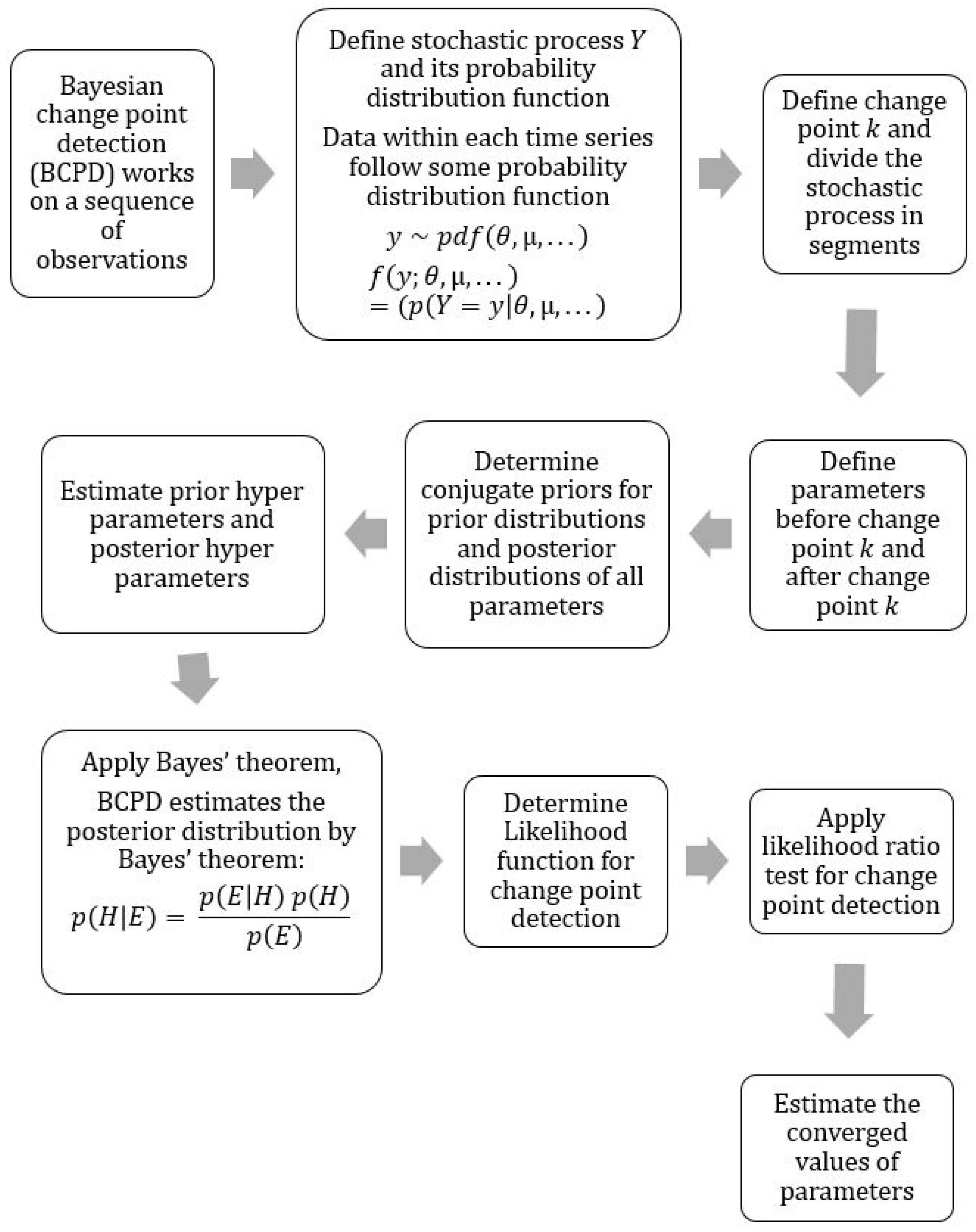
Figure 1. Flowchart for change point (k) detection.
Mathematics 07 00474 g001
Figure 2. CUSUM chart for Guro P M 2.5 .
Mathematics 07 00474 g002
Figure 3. CUSUM chart for Guro P M 10 .
Mathematics 07 00474 g003
Figure 4. CUSUM chart for Nowon P M 2.5 .
Mathematics 07 00474 g004
Figure 5. CUSUM chart for Nowon P M 10 .
Mathematics 07 00474 g005
Figure 6. CUSUM chart for Songpa P M 2.5 .
Mathematics 07 00474 g006
Figure 7. CUSUM chart for Songpa P M 10 .
Mathematics 07 00474 g007
Figure 8. CUSUM chart for Yongsan P M 2.5 .
Mathematics 07 00474 g008
Figure 9. CUSUM chart for Yongsan P M 10 .
Mathematics 07 00474 g009
Figure 10. CUSUM chart for Guro P M 2.5 plus 10 bootstraps (European Standards).
Mathematics 07 00474 g010
Figure 11. CUSUM chart for Guro P M 10 plus 10 bootstraps (European Standards).
Mathematics 07 00474 g011
Figure 12. CUSUM chart for Nowon P M 2.5 plus 10 bootstraps (European Standards).
Mathematics 07 00474 g012
Figure 13. CUSUM chart for Nowon P M 10 plus 10 bootstraps (European Standards).
Mathematics 07 00474 g013
Figure 14. CUSUM chart for Songpa P M 2.5 plus 10 bootstraps (European Standards).
Mathematics 07 00474 g014
Figure 15. CUSUM chart for Songpa P M 10 plus 10 bootstraps (European Standards).
Mathematics 07 00474 g015
Figure 16. CUSUM chart for Yongsan P M 2.5 plus 10 bootstraps (European Standards).
Mathematics 07 00474 g016
Figure 17. CUSUM chart for Yongsan P M 10 plus 10 bootstraps (European Standards).
Mathematics 07 00474 g017
Figure 18. Guro (Seoul, South Korea) monthly polluted days before and after the change point due to P M 2.5 .
Mathematics 07 00474 g018
Figure 19. Guro (Seoul, South Korea) monthly polluted days before and after the change point due to P M 10 .
Mathematics 07 00474 g019
Figure 20. Nowon (Seoul, South Korea) monthly polluted days before and after the change point due to P M 2.5 .
Mathematics 07 00474 g020
Figure 21. Nowon (Seoul, South Korea) monthly polluted days before and after the change point due to P M 10 .
Mathematics 07 00474 g021
Figure 22. Songpa (Seoul, South Korea) monthly polluted days before and after the change point due to P M 2.5 .
Mathematics 07 00474 g022
Figure 23. Songpa (Seoul, South Korea) monthly polluted days before and after the change point due to P M 10 .
Mathematics 07 00474 g023
Figure 24. Yongsan (Seoul, South Korea) monthly polluted days before and after the change point due to P M 2.5 .
Mathematics 07 00474 g024
Figure 25. Yongsan (Seoul, South Korea) monthly polluted days before and after the change point due to P M 10 .
Mathematics 07 00474 g025
Table 1. Author’s contribution in the direction of research.
AuthorsAirborne Particulate Matters
( PM 2.5 , PM 10 )
Change-Point DetectionBCPD
(Bayesian Change Point Detection)
Time Series Analysis
Lim et al. (2012) [28]Ambient particulate matter (PM)---
Rao et al. (2018) [29]Particulate matter air pollution---
Wei and Meng (2018) [30]Airborne fine particulate matter ( P M 2.5 )---
Wang et al. (2017) [31]Inhaled particulate matter---
Heroux et al. (2015) [1]Ambient air pollutants---
Wellenius et al. (2012) [32]Ambient Air Pollution---
Pirani et al. (2015) [4]Airborne particles--Bayesian inference within Time series
Li et al. (2013) [33]Airborne particulate matter--Time series analysis
Kim et al. (2018a) [34]Particulate matter---
Kim et al. (2017) [35]Air pollution--Time series model
Qin et al. (2017) [36]Air pollution--Time series analysis
Lee et al. (2015) [37]Fine and coarse particles--Time series analysis
Cabrieto et al. (2018) [38]-kernel change point detection, correlation changes--
Keshavarz et al. (2018) [7] Generalized likelihood ratio test,--
-One-dimensional Gaussian process--
Kucharczyk et al. (2018) [8]-likelihood ratio test,--
fractional Brownian motion--
Lu et al. (2017) [9]-Change-point detection, machine monitoring,--
Anomaly measure (AR model), Martingale testTime series data
-On-line change detection,--
Hilgert et al. (2016) [12]-autoregressive dynamic models,--
-CUSUM-like scheme--
Górecki et al. (2017) [13]-Change point detection, heteroscedastic,-Time series data
-Karhunen-Loeve expansions--
-Change point detection, bootstrap, Time series data
Bucchia and Wendler (2017) [14]-Hilbert space valued random fields,--
-(Cramer–von Mises type test)--
Zhou et al. (2015) [16]-Sequential change point detection,--
-linear quantile regression models--
Lu and Chang (2016) [17]-Detecting change points,--
-mean/variance shifts, FCML-CP algorithm--
Liu et al. (2013) [11]-Change point detection, Time series analysis
-relative density ratio estimation--
Ruggieri and Antonellis (2016) [19]--Bayesian sequential change point detection-
Keshavarz and Huang (2014) [20]--Bayesian and Expectation Maximization methods,
--multivariate change point detection-
Kurt et al. (2018) [21]--Bayesian change point model,-
--SIP-based DDoS attacks detection-
--Post classification change detection,-
Wu et al. (2017) [22]--iterative slow feature analysis,-
--Bayesian soft fusion-
Gupta and Baker (2017) [26]--Spatial event rates, change point,
--Bayesian statistics, induced seismicity-
Marino et al. (2017) [23]--Change point, multiple biomarkers,-
--ovarian cancer-
Jeon et al. (2016) [24]--Abrupt change point detection,-
--annual maximum precipitation, fused lasso-
Bardwell and Fearnhead (2017) [27]--Bayesian Detection, Abnormal SegmentsTime series analysis
Chen et al. (2017) [25]--Bayesian change point analysis,-
--extreme daily precipitation-
This studyAirbone Particulate MatterChange point detectionBayesian approach and likelihood ratio test for change point detectionTime series data
Table 2. Change point detection.
AuthorsChange-Point Detection
Cabrieto et al. (2018) [38]Detection of correlation changes by applying kernel change point detection on the running correlations
Keshavarz et al. (2018) [7]Detecting a change in the mean of one-dimensional Gaussian process data in the fixed domain regime based on the generalized likelihood ratio test (GLRT)
Kucharczyk et al. (2018) [8]Variance change point detection for fractional Brownian motion based on the likelihood ratio test
Lu et al. (2017) [9]Graph-based structural change detection for rotating machinery monitoring by martingale-test method
Hilgert et al. (2016) [12]On-line change detection for uncertain autoregressive dynamic models through nonparametric estimation (CUSUM-like scheme)
Górecki et al. (2017) [13]Change point detection in heteroscedastic time series through Karhunen-Loeve expansions
Bucchia and Wendler (2017) [14]Change point detection and bootstrap for Hilbert space valued random fields (Cramer-von Mises type test)
Zhou et al. (2015) [16]A method for sequential detection of structural changes in linear quantile regression models.
Lu and Chang (2016) [17]Detecting change-points for shifts in mean and variance using fuzzy classification maximum likelihood change-point (FCML-CP) algorithm
Liu et al. (2013) [11]Change point detection in time-series data by relative density-ratio estimation
This studyChange point detection for airborne particulate matter ( P M 2.5 , P M 10 ) through Bayesian approach and likelihood ratio test
Table 3. BCPD (Bayesian change point detection).
AuthorsBCPD (Bayesian Change Point Detection)
Ruggieri and Antonellis (2016) [19]A sequential Bayesian change point algorithm was proposed that provides uncertainty bounds on both the number and location of change points
Keshavarz and Huang (2014) [20]Bayesian and Expectation Maximization (EM) methods for change point detection problem of multivariate data with both single and multiple changes
Kurt et al. (2018) [21]A Bayesian change point model for detecting SIP-based DDoS attacks
Wu et al. (2017) [22]A post-classification change detection method based on iterative slow feature analysis and Bayesian soft fusion
Gupta and Baker (2017) [26]Estimating spatially varying event rates with a change point using Bayesian statistics: Application to induced seismicity
Marino et al. (2017) [23]Change-point of multiple biomarkers in women with ovarian cancer
Jeon et al. (2016) [24]Abrupt change point detection of annual maximum precipitation through fused lasso penalty function by using the Generalized Extreme Value (GEV) distribution
Bardwell and Fearnhead (2017) [27]Bayesian Detection of Abnormal Segments in Multiple Time Series
Chen et al. (2017) [25]Bayesian change point analysis for extreme daily precipitation
This studyChange point detection for airborne particulate matter ( P M 2.5 , P M 10 ) through Bayesian approach and likelihood ratio test
Table 4. Region-wise air quality standards for particulate matters ( P M 2.5 and P M 10 ).
Air Quality Standards for PM 2.5
( μ g/m 3 )
Air Quality Standards for PM 10
( μ g/m 3 )
European Standard ( P M 2.5 )25European Standard ( P M 10 ) 24 h50
American Standard ( P M 2.5 )35American Standard ( P M 10 ) 24 h150
Korean Standard ( P M 2.5 ) 24 h50Korean Standard ( P M 10 ) 24 h100
Table 5. Particulate matter ( P M 2.5 ) location-wise data.
Particle PollutionCriteria ( μ g/m 3 )Total Number of DaysEffective ReadingsDangerous Concentration%Age against Total Days%Age against Effective Readings
P M 2.5 Guro’s data (Seoul, South Korea)
European Standard2524982486112545.04%45.25%
American Standard352498248653221.30%21.40%
Korean Standard50249824862078.29%8.33%
P M 2.5 Nowon’s data (Seoul, South Korea)
European Standard2532283031137142.47%45.23%
American Standard353228303171822.24%23.69%
Korean Standard50322830312557.90%8.41%
P M 2.5 Songpa’s data (Seoul, South Korea)
European Standard2536533388154742.35%45.66%
American Standard353653338879521.76%23.47%
Korean Standard50365333882817.69%8.29%
P M 2.5 Yongsan’s data (Seoul, South Korea)
European Standard2536533456153742.08%44.47%
American Standard353653345674620.42%21.59%
Korean Standard50365334562807.66%8.10%
Table 6. Particulate matter ( P M 10 ) location-wise data.
Particle PollutionCriteria ( μ g/m 3 )Total Number of DaysEffective ReadingsDangerous Concentration%Age against Total Days%Age against Effective Readings
P M 10 Guro’s data (Seoul, South Korea)
European Standard5036533540158043.25%44.63%
American Standard15036533540601.64%1.69%
Korean Standard100365335402797.64%7.88%
P M 10 Nowon’s data (Seoul, South Korea)
European Standard5036533531144439.53%40.89%
American Standard15036533531411.12%1.16%
Korean Standard100365335312396.54%6.77%
P M 10 Songpa’s data (Seoul, South Korea)
European Standard5036533467149040.79%42.98%
American Standard15036533467501.37%1.44%
Korean Standard100365334672406.57%6.92%
P M 10 Yongsan’s data (Seoul, South Korea)
European Standard5036533508156642.87%44.64%
American Standard15036533508601.64%1.71%
Korean Standard100365335082827.72%8.04%
Table 7. P M 2.5 Poisson Process.
PM 2.5 Poisson Process (Rate) θ
AreaDistributionEuropean StandardsAmerican StandardsKorean Standards
GuroPoisson13.7206.4882.524
NowonPoisson12.9346.7742.406
SongpaPoisson12.8926.6252.342
YongsanPoisson12.8086.2172.333
Table 8. P M 10 Poisson Process.
PM 10 Poisson Process (Rate) θ
AreaDistributionEuropean StandardsAmerican StandardsKorean Standards
GuroPoisson13.1670.5002.325
NowonPoisson12.0330.3421.992
SongpaPoisson12.4170.4172.000
YongsanPoisson13.0500.5002.350
Table 9. P M 2.5 Converged values of parameters (Bayesian approach).
PM 2.5 Converged Values of Parameters (Bayesian Approach)
Replication MeanGuroNowonSongpaYongsan
( θ )
Replication Mean
( λ )
Replication Mean
K
Replication Mean
( θ )
Replication Mean
( λ )
Replication Mean
K
Replication Mean
( θ )
Replication Mean
( λ )
Replication Mean
K
Replication Mean
( θ )
Replication Mean
( λ )
Replication Mean
K
Replication Mean
European standards
V 1 15.9611.1743.2915.8810.3049.9814.9311.2453.6924.8012.136.92
V 2 16.0311.2542.5315.8910.3449.8314.9011.2853.8124.4612.158.07
V 3 16.0011.1843.1215.9010.3249.7614.9111.2553.9224.8112.077.49
V 4 16.0111.1743.1915.9010.3049.9614.9111.2454.0524.7712.147.75
V 5 15.9811.1243.5215.8810.2650.1314.9311.2353.5924.5612.097.48
V 6 15.9611.1443.6115.8710.2850.1214.8911.2453.9824.0712.089.48
V 7 15.9511.1743.4115.8410.3050.1214.8811.2653.9124.6112.038.20
V 8 16.0411.2142.7615.9410.3449.6514.9311.2653.7324.6912.137.87
V 9 16.0111.1942.7515.8810.3049.7814.9011.2453.7124.5012.107.83
V 10 15.9611.1543.5915.8510.3050.2314.8811.2554.0724.2312.128.30
( V ) Mean of 10 replications15.9911.1743.1815.8810.3049.9514.9011.2553.8524.5512.107.94
American standards
V 1 8.355.3233.469.824.7742.118.734.9553.3216.125.696.17
V 2 8.245.3333.679.844.8041.768.724.9653.3116.045.716.17
V 3 8.225.3034.319.824.7842.128.724.9553.3516.005.696.21
V 4 8.295.3034.109.844.7941.758.724.9553.3216.085.686.18
V 5 8.315.3033.499.864.7741.678.724.9353.3216.055.676.17
V 6 8.275.3133.709.804.7742.118.714.9453.3915.965.686.20
V 7 8.245.3034.019.884.7941.668.704.9553.3315.925.696.19
V 8 8.255.3233.709.864.8041.618.744.9653.2516.165.696.16
V 9 8.475.3332.469.834.7841.668.724.9453.2115.995.686.16
V 10 8.385.3333.289.824.7941.898.714.9553.4215.965.696.21
( V )
Mean of 10 replications
8.305.3133.629.844.7841.838.724.9553.3216.035.696.18
Korean standards
V 1 3.581.6338.143.751.2150.293.131.6456.577.952.055.80
V 2 3.571.6537.903.741.2250.253.151.6556.267.952.065.76
V 3 3.581.6437.973.751.2150.233.151.6456.347.922.055.80
V 4 3.571.6238.403.741.2050.433.151.6356.548.012.065.77
V 5 3.561.6138.483.741.2050.323.141.6356.507.942.055.78
V 6 3.551.6238.633.731.2050.523.131.6356.877.972.045.77
V 7 3.541.6238.603.751.2050.303.131.6456.537.872.055.80
V 8 3.591.6437.933.751.2150.273.161.6456.087.982.065.78
V 9 3.571.6337.843.731.2050.433.151.6455.867.902.055.79
V 10 3.551.6238.693.731.2150.363.131.6356.867.902.055.79
( V )
Mean of 10 replications
3.561.6338.263.741.2150.343.141.6456.447.942.055.78
Table 10. P M 10 Converged values of parameters (Bayesian approach).
PM 10 Converged Values of Parameters (Bayesian Approach)
Replication MeanGuroNowonSongpaYongsan
( θ )
Replication Mean
( λ )
Replication Mean
K
Replication Mean
( θ )
Replication Mean
( λ )
Replication Mean
K
Replication Mean
( θ )
Replication Mean
( λ )
Replication Mean
K
Replication Mean
( θ )
Replication Mean
( λ )
Replication Mean
K
Replication Mean
European standards
V 1 14.719.2085.5314.958.3667.0416.119.4953.2914.578.4190.09
V 2 14.759.2785.1014.938.3967.1016.089.5253.3014.578.5089.53
V 3 14.749.2085.4914.938.3667.1616.119.4553.2914.588.4789.63
V 4 14.759.1985.4714.938.3567.1716.089.4753.5214.578.3990.16
V 5 14.769.1285.6514.928.3367.1316.069.4453.7514.568.3589.85
V 6 14.729.1885.5914.918.3567.2016.069.4753.4314.548.4289.98
V 7 14.719.1885.7514.908.3667.1316.149.4853.3614.528.4190.12
V 8 14.779.2585.0714.968.3767.0516.089.3953.9314.618.5189.23
V 9 14.739.1885.2914.928.3567.0316.079.4753.2614.608.4888.67
V 10 14.729.1985.6714.918.3767.1616.039.4653.9114.538.3990.18
( V )
Mean of 10 replications
14.739.2085.4614.938.3667.1216.089.4653.5014.568.4389.74
American standards
V 1 0.630.1290.650.690.1366.560.560.0787.630.660.0491.61
V 2 0.630.1290.760.630.1172.520.550.0789.080.660.0491.33
V 3 0.630.1290.670.520.0881.790.560.0787.860.660.0491.46
V 4 0.630.1290.340.530.0981.320.570.0786.800.660.0491.41
V 5 0.630.1290.230.760.1460.700.560.0688.350.670.0491.03
V 6 0.630.1290.480.520.0881.910.560.0787.980.660.0491.50
V 7 0.630.1290.530.450.0689.850.560.0688.720.660.0591.18
V 8 0.630.1290.630.820.1556.420.560.0988.730.660.0491.11
V 9 0.630.1389.330.640.1171.370.560.0788.190.660.0491.69
V 10 0.640.1289.790.590.1175.610.560.0788.260.660.0491.29
( V )
Mean of 10 replications
0.630.1290.340.620.1173.800.560.0788.160.660.0491.36
Korean standards
V 1 2.890.9185.252.920.8965.683.161.0952.783.321.1167.44
V 2 2.900.9285.172.910.8965.673.171.1052.653.331.1366.93
V 3 2.890.9085.962.920.8965.693.171.0952.793.321.1267.52
V 4 2.880.8886.672.910.8865.693.171.0952.833.301.0868.72
V 5 2.900.9184.972.910.8865.673.161.0852.793.301.0968.37
V 6 2.880.8986.132.910.8865.723.161.0952.753.271.0669.89
V 7 2.870.8787.122.900.8965.703.161.0952.643.281.0868.93
V 8 2.890.8986.142.920.8865.673.181.0952.593.331.1267.09
V 9 2.880.8986.272.900.8865.633.161.0952.563.311.1067.66
V 10 2.880.9086.172.900.8965.743.151.0953.153.301.1068.08
( V )
Mean of 10 replications
2.890.9085.982.910.8965.683.161.0952.753.311.1068.06
Table 11. P M 2.5 Change Point (k) for European, American and Korean Standards through Bayesian approach.
Bayesian Approach for Change Point Detection
Area Seoul, South Korea ( θ )
Rate before Change Point
( λ )
Rate after Change Point
K Change Point R θ
Convergence Parameter for ( θ )
Var ( V ) θ
Variance for ( θ )
R λ
Convergence Parameter for ( λ )
Var ( V ) λ
Variance for ( λ )
R K
Convergence Parameter for K
Var ( V ) K
Variance for K
European standards
Guro15.9911.1743.181.0004080.5831.0007190.5411.00074759.219
Nowon15.8810.3049.950.9999430.7831.0000940.4721.00003634.238
Songpa14.9011.2553.851.0001990.3021.0000070.1801.0008709.719
Yongsan24.5512.107.941.00089821.9611.0009430.4771.00203190.053
American standards
Guro8.305.3133.621.0025401.0641.0001050.1761.00125675.773
Nowon9.844.7841.831.0005950.2961.0002000.0891.00115913.007
Songpa8.724.9553.320.9998570.1720.9999340.0761.0002552.395
Yongsan16.035.696.180.9999935.7260.9999560.1011.0000280.356
Korean standards
Guro3.561.6338.261.0004750.1321.0004390.0521.00086541.605
Nowon3.741.2150.340.9999590.0831.0003770.0250.9999789.024
Songpa3.141.6456.441.0002000.0681.0001440.0311.00058845.887
Yongsan7.942.055.781.0001361.4981.0002370.0180.9997800.339
Table 12. P M 2.5 Last point before change (k) and First point after change ( k + 1 ) for European, American and Korean Standards through CUSUM approach.
CUSUM Approach for Change Point Detection
Area Seoul, South Korea ( θ )
Average Rate before Change
( λ )
Average Rate after Change
K
Last Point before Change
k + 1
First Point after Change
S m
Most Extreme Point
S max
Highest Point in CUSUM
S min
Lowest Point in CUSUM
S diff
Magnitude of Change
Confidence
Level %
European standards
Guro16.2311.334041100.22100.220−5.280105.500100%
Nowon15.8110.065354152.50152.500−3.066155.566100%
Songpa14.9811.245354110.74110.742−6.108116.850100%
Yongsan20.6412.02111286.1186.108−5.19291.30070%
American standards
Guro8.145.20363759.4459.439−5.02464.463100%
Nowon9.904.804142128.28128.283−3.321131.604100%
Songpa8.794.975253112.50112.500−5.375117.875100%
Yongsan7.314.96646570.1370.133−4.78374.917100%
Korean standards
Guro3.691.66353640.6540.646−1.47642.122100%
Nowon3.761.20505167.7267.717−5.21772.934100%
Songpa3.231.66525346.2346.233−8.27554.508100%
Yongsan3.031.54646544.6744.667−1.66746.333100%
Table 13. P M 10 Change Point (k) for European, American and Korean Standards.
Bayesian Approach for Change Point Detection
Area Seoul, South Korea ( θ )
Rate before Change Point
( λ )
Rate after Change Point
K Change Point R θ
Convergence Parameter for ( θ )
Var ( V ) θ
Variance for ( θ )
R λ
Convergence Parameter for ( λ )
Var ( V ) λ
Variance for ( λ )
R K
Convergence Parameter for K
Var ( V ) K
Variance for K
European standards
Guro14.739.2085.461.0000720.4251.0004270.9250.99993164.845
Nowon14.938.3667.120.9998790.4640.9999250.3271.0000403.184
Songpa16.089.4653.501.0003000.6431.0012820.3101.0033639.133
Yongsan14.568.4389.741.0001230.5971.0004371.4921.00109475.750
American standards
Guro0.630.1290.340.9998400.0091.0003200.0051.00282131.264
Nowon0.620.1173.801.0411870.1731.0363550.0111.0535741089.508
Songpa0.560.0788.161.0001350.0161.0002530.0371.000710174.232
Yongsan0.660.0491.360.9998510.0161.0002960.0041.00021932.243
Korean standards
Guro2.890.9085.981.0008200.0461.0015760.0531.00342959.252
Nowon2.910.8965.680.9998810.0451.0001370.0161.0003380.567
Songpa3.161.0952.750.9999350.0661.0000750.0171.0014457.194
Yongsan3.311.1068.061.0022090.0771.0037090.0501.00478781.344
Table 14. P M 10 Last point before change (k) and First point after change ( k + 1 ) for European, American and Korean Standards through CUSUM approach.
CUSUM Approach for Change Point Detection
Area Seoul, South Korea ( θ )
Average Rate before Change
( λ )
Average Rate after Change
K
Last point before Change
k + 1
First Point after Change
S m
Most Extreme Point
S max
Highest Point in CUSUM
S min
Lowest Point in CUSUM
S diff Magnitude of ChangeConfidence Level %
European standards
Guro15.059.797778145.17145.167−0.833146.000100%
Nowon14.978.326768196.77196.767−2.967199.733100%
Songpa16.159.465354197.92197.917−1.583199.500100%
Yongsan15.019.537778151.15151.150−1.950153.100100%
American standards
Guro0.640.10899012.5012.500−2.00014.500100%
Nowon0.510.16636410.4810.4750.00010.47580%
Songpa0.700.19535414.9214.917−5.83320.750100%
Yongsan0.670.00899015.5015.500−0.50016.00010%
Korean standards
Guro3.201.32646556.2056.200−0.67556.875100%
Nowon2.910.87666760.5560.550−1.00861.558100%
Songpa3.191.09525362.0062.000−4.00066.000100%
Yongsan3.391.16646566.6066.600−0.65067.250100%