Evaluation of Fractional Integrals and Derivatives of Elementary Functions: Overview and Tutorial

Abstract

Several fractional-order operators are available and an in-depth knowledge of the selected operator is necessary for the evaluation of fractional integrals and derivatives of even simple functions. In this paper, we reviewed some of the most commonly used operators and illustrated two approaches to generalize integer-order derivatives to fractional order; the aim was to provide a tool for a full understanding of the specific features of each fractional derivative and to better highlight their differences. We hence provided a guide to the evaluation of fractional integrals and derivatives of some elementary functions and studied the action of different derivatives on the same function. In particular, we observed how Riemann–Liouville and Caputo’s derivatives converge, on long times, to the Grünwald–Letnikov derivative which appears as an ideal generalization of standard integer-order derivatives although not always useful for practical applications.

1. Introduction

Fractional calculus, the branch of calculus devoted to the study of integrals and derivatives of non integer order, is nowadays extremely popular due to a large extent of its applications to real-life problems (see, for instance, [1,2,3,4,5,6,7,8]).

Although this subject is as old as the more classic integer-order calculus, its development and diffusion mainly started to take place no more than 20 or 30 years ago. As a consequence, several important results in fractional calculus are still not completely known or understood by non-specialists, and this topic is usually not taught in undergraduate courses.

The presence of more than one type of fractional derivative is sometimes a source of confusion and it is not occasional to find wrong or not completely rigorous results in distinguished journals as well. Even the simple evaluation of a fractional integral or derivative of elementary functions is in some cases not reported in a correct way, which is also due to the difficulty of properly handling the different operators.

For instance, in regards to the exponential, the sine and the cosine functions, the usual and well-known relationships:

$$\frac{{\mathrm{d}}^n}{\mathrm{d}{t}^n}{\mathrm{e}}^{t\Omega }={\Omega }^n{\mathrm{e}}^{t\Omega },\frac{{\mathrm{d}}^n}{\mathrm{d}{t}^n}sint\Omega ={\Omega }^{n}sin\left(t\Omega +\frac{n\pi }{2}\right),\frac{{\mathrm{d}}^n}{\mathrm{d}{t}^n}cost\Omega ={\Omega }^{n}cos\left(t\Omega +\frac{n\pi }{2}\right),$$

(1)

which hold for any $n\in \mathbb{N}$ and turn out extremely useful for simplifying a lot of mathematical derivations, are in general no longer true with fractional derivatives, unless a very special definition is used, which presents some not secondary drawbacks.

The main aim of this paper is to provide a tutorial for the evaluation of fractional integrals and derivatives of some elementary functions and to show the main differences resulting from the action of different types of fractional derivatives. At the same time, we present an alternative perspective for the derivation of some of the most commonly used fractional derivatives in order to help the reader to better interpret the results obtained from their application.

In particular, the more widely used definitions of fractional derivatives, namely those known as Grünwald–Letnikov, Riemann–Liouville and Caputo, are introduced according to two approaches: One based on the inversion of the generalization of the integer-order integral and the other based on the more direct generalization of the limit of the difference quotients defining integer-order derivatives. Although they lead to equivalent results, the second and less usual approach allows for a more comprehensive understanding of the nature of the different operators and a better explanation of the effects produced on elementary functions. In particular we will observe when relationships similar to Equation (1) apply to fractional derivatives and the way in which fractional derivatives deviate from Equation (1).

Some of the material presented in this paper is clearly not new (proper references will be given through the paper). Nevertheless, we think that it is important to collect in a single paper a series of results which are scattered among several references or are not clearly exposed, thus to provide a systematic treatment and a guide for researchers approaching fractional calculus for the first time.

The paper is organized as follows: In Section 2 we recall the fractional Riemann–Liouville integral and some definitions of fractional derivatives relying on its inversion. We hence present in Section 3 a different view of the same definitions by showing, in a step-by-step way, how they can be obtained as a generalization of the limit of different quotients defining standard integer-order derivatives after operating a replacement of the function to cope with convergence difficulties. Since the Mittag–Leffler (ML) function plays an important role in fractional calculus, and indeed most of the results on derivatives of elementary functions will be based on this function, Section 4 is devoted to present this function and some of its main properties; in particular, we provide a useful result on the asymptotic behavior of the ML function which allows to investigate the relationships between the action of the different fractional derivatives on the same function. Section 5, Section 6 and Section 7 are devoted to presenting the evaluation of derivatives of some elementary functions (power, exponential and sine and cosine functions), to study their properties and to highlight the different effects of the various operators. Clearly the results on the few elementary functions considered in this paper may be adopted as a guide to extend the investigation to further and more involved functions. Some concluding remarks are finally presented in Section 8.

2. Fractional Derivatives as Inverses of the Fractional Riemann–Liouville Integral

To simplify the reading of this paper we recall in this Section the most common definitions in fractional calculus and review some of their properties. For a more comprehensive introduction to fractional integrals and fractional derivatives we refer the reader to any of the available textbooks [3,5,9,10,11,12] or review papers [13,14]. In particular, we follow here the approach based on the generalization, to any real positive order, of standard integer-order integrals and on the introduction of fractional derivatives as their inverse operators. We therefore start by recalling the well-known definition of the fractional Riemann–Liouville (RL) integral.

Definition 1.

For a function $f\in L^1\left([t_0,T]\right)$ the RL integral of order $\alpha >0$ and origin $t_0$ is defined as:

$$J_{t_0}^{\alpha }f\left(t\right)=\frac{1}{\Gamma \left(\alpha \right)}{\int }_{t_0}^t{(t-\tau )}^{\alpha -1}f\left(\tau \right)\mathrm{d}\tau ,\forall t\in (t_0,T].$$

(2)

As usual, $L^1\left([t_0,T]\right)$ denotes the set of Lebesgue integrable functions on $[t_0,T]$ and $\Gamma \left(x\right)$ is the Euler gamma function

$$\Gamma \left(x\right)={\int }_0^{\infty }{t}^{x-1}{\mathrm{e}}^{-t}\mathrm{d}t,$$

(3)

a function playing an important role in fractional calculus since it generalizes the factorial to real arguments; it is indeed possible to verify that $\Gamma (x+1)=x\Gamma \left(x\right)$ and hence, since $\Gamma \left(1\right)=1$, it is:

$$\Gamma (n+1)=n!\mathrm{for}\mathrm{any}n\in \mathbb{N}.$$

It is due to the above fundamental property of the Euler gamma function that the RL integral (2) can be viewed as a straightforward extension of standard n-fold repeated integrals:

$${\int }_{t_0}^t{\int }_{t_0}^{{\tau }_1}\cdots {\int }_{t_0}^{{\tau }_{n-1}}f\left({\tau }_n\right)\mathrm{d}{\tau }_n\cdots \mathrm{d}{\tau }_2\mathrm{d}{\tau }_1=\frac{1}{(n-1)!}{\int }_{t_0}^t{(t-\tau )}^{n-1}f\left(\tau \right)\mathrm{d}\tau$$

where it is sufficient to replace the integer n with any real $\alpha >0$ to obtain RL integral (2).

In the special case of the starting point $t_0\to -\infty$ the integral on the whole real axis:

$$J_{-\infty }^{\alpha }f\left(t\right)=\underset{t_0\to -\infty }{lim}{J}_{t_0}^{\alpha }f\left(t\right)=\frac{1}{\Gamma \left(\alpha \right)}{\int }_{-\infty }^t{(t-\tau )}^{\alpha -1}f\left(\tau \right)\mathrm{d}\tau ,t\in \mathbb{R},$$

(4)

is usually referred to as the Liouville (left-sided) fractional integral (see [12] (Chapter 5) or [10] (§2.3)) and satisfies similar properties as the integer-order integral, such as $J_{-\infty }^{\alpha }{\mathrm{e}}^{\Omega t}={\Omega }^{-\alpha }{\mathrm{e}}^{\Omega t}$.

Once a robust definition for fractional-order integrals is available, as the RL integral (2), fractional derivatives can be introduced as their left-inverses in a similar way as standard integer-order derivatives are the inverse operators of the corresponding integrals.

To this purpose let us denote with $m=⌈\alpha ⌉$ the smallest integer greater or equal to $\alpha$ and, since $m-\alpha >0$, consider the RL integral $J_{t_0}^{m-\alpha }$. Thanks to the semigroup property $J_{t_0}^{m-\alpha }{J}_{t_0}^{\alpha }f\left(t\right)=J_{t_0}^{m}f\left(t\right)$ [9] (Theorem 2.1) which returns an integer-order integral, it is sufficient to apply the integer-order derivative $D^m$ to obtain the identity:

$$D^m{J}_{t_0}^{m-\alpha }{J}_{t_0}^{\alpha }f\left(t\right)=D^m{J}_{t_0}^{m}f\left(t\right)=f\left(t\right);$$

the concatenation $D^m{J}_{t_0}^{m-\alpha }$ hence provides the left-inverse of $J_{t_0}^{\alpha }$ and therefore justifies the following definition of the RL fractional derivative.

Definition 2.

Let $\alpha >0$, $m=⌈\alpha ⌉$ and $t_0\in \mathbb{R}$. The RL fractional derivative of order α and starting point $t_0$ is:

$${}^{\mathit{RL}}{D}_{t_0}^{\alpha }f\left(t\right):=D^m{J}_{t_0}^{m-\alpha }f\left(t\right)=\frac{1}{\Gamma (m-\alpha )}\frac{{\mathrm{d}}^m}{\mathrm{d}{t}^m}{\int }_{t_0}^t{(t-\tau )}^{m-\alpha -1}f\left(\tau \right)\mathrm{d}\tau ,t>t_0.$$

(5)

The RL derivative (5) is not the only left inverse of $J_{t_0}^{\alpha }$ and in applications, a different operator is usually preferred. One of the major drawbacks of the RL derivative is that it requires to be initialized by means of fractional integrals and fractional derivatives. To fully understand this issue it is useful to consider the following result on the Laplace transform (LT) of the RL derivative [10].

Proposition 1.

Let $\alpha >0$ and $m=⌈\alpha ⌉$. The LT of the RL derivative of a function $f\left(t\right)$ is:

$$\mathcal{L}\left({}^{\mathit{RL}}{D}_{t_0}^{\alpha }f\left(t\right);s\right)=s^{\alpha }F\left(s\right)-\sum _{j=1}^{m-1}{s}^{m-1-j}{}^{\mathit{RL}}{D}_{t_0}^{\alpha -m+j}f\left(t\right){|}_{t=t_0^{+}}-s^{m-1}{J}_{t_0}^{m-\alpha }f\left(t\right){|}_{t=t_0^{+}},$$

with $F\left(s\right)$ the LT of $f\left(t\right)$.

A consequence of this result is that fractional differential equations (FDEs) with the RL derivative need to be initialized with the same kind of values. The uniqueness of the solution $y\left(t\right)$ of a FDE requires that initial conditions on $J_{t_0}^{m-\alpha }y\left(t\right){|}_{t=t_0^{+}}$ and ${}^{\mathrm{RL}}{D}_{t_0}^{\alpha -m+j}y\left(t\right){|}_{t=t_0^{+}}$, $j=1,\dots ,m-1$, are assigned (e.g., see [9] (Theorem 5.1) or [10] (Chapter 3)).

In the majority of applications, however, these values are not available because they do not have a clear physical meaning and therefore the description of the initial state of a system is quite difficult when the RL derivative is involved. This is one of the reasons which motivated the introduction of the alternative fractional Caputo’s derivative obtained by simply interchanging differentiation and integration in RL Derivative (5).

Definition 3.

Let $\alpha >0$, $m=⌈\alpha ⌉$ and $t_0\in \mathbb{R}$. For a function $f\in A^m\left([t_0,T]\right)$, i.e., such that $f^{(m-1)}$ is absolutely continuous, the Caputo’s derivative is defined as:

$${}^C{D}_{t_0}^{\alpha }f\left(t\right):=J_{t_0}^{m-\alpha }{D}^{m}f\left(t\right)=\frac{1}{\Gamma (m-\alpha )}{\int }_{t_0}^t{(t-\tau )}^{m-\alpha -1}{f}^{\left(m\right)}\left(\tau \right)\mathrm{d}\tau ,t>t_0,$$

(6)

where $D^m$ and $f^{\left(m\right)}$ denote integer-order derivatives.

Unlike the RL derivative, the LT of the Caputo’s derivative is initialized by standard initial values expressed in terms of integer-order derivatives, as summarized in the following result [9].

Proposition 2.

Let $\alpha >0$ and $m=⌈\alpha ⌉$. The LT of the Caputo’s derivative of a function $f\left(t\right)$ is:

$$\mathcal{L}\left({}^C{D}_{t_0}^{\alpha }f\left(t\right);s\right)=s^{\alpha }F\left(s\right)-\sum _{j=0}^{m-1}{s}^{\alpha -1-j}{f}^{\left(j\right)}\left(t_0\right),$$

with $F\left(s\right)$ the LT of $f\left(t\right)$.

It is a clear consequence of the above result that FDEs with the Caputo’s derivative require, to ensure the uniqueness of the solution $y\left(t\right)$, the assignment of initial conditions in the more traditional Cauchy form $y^{\left(j\right)}\left(t_0\right)=y_{0,j}$, $j=0,1,\dots ,m-1$, thus allowing a more convenient application to real-life problems.

Although different, the Caputo’s derivative shares with the RL derivative the property of being the left inverse of the RL integral since ${}^{\mathrm{C}}{D}_{t_0}^{\alpha }{J}_{t_0}^{\alpha }f=f$ [9] (Theorem 3.7). However, ${}^{\mathrm{C}}{D}_{t_0}^{\alpha }$ is not the right inverse of $J_{t_0}^{\alpha }$ since [9] (Theorem 3.8),

$$J_{t_0}^{\alpha }{}^{\mathrm{C}}{D}_{t_0}^{\alpha }f\left(t\right)=f\left(t\right)-T_{m-1}[f;t_0]\left(t\right),$$

(7)

where $T_{m-1}[f;t_0]\left(t\right)$ is the Taylor polynomial of f centered at $t_0$,

$$T_{m-1}[f;t_0]\left(t\right)=\sum _{k=0}^{m-1}\frac{{(t-t_0)}^k}{k!}{f}^{\left(k\right)}\left(t_0\right).$$

(8)

The polynomial $T_{m-1}[f;t_0]\left(t\right)$ is important for establishing the relationship between fractional derivatives of RL and Caputo type. After differentiating both sides of Formula (7) in the RL sense it is possible to derive:

$${}^{\mathrm{C}}{D}_{t_0}^{\alpha }f\left(t\right)={}^{\mathrm{RL}}{D}_{t_0}^{\alpha }\left(f\left(t\right)-T_{m-1}[f;t_0]\left(t\right)\right).$$

(9)

Although several other definitions of fractional integrals and derivatives have been introduced in the last years, we confine our treatment to the above operators which are the most popular; the utility and the nature of some of the operators recently proposed is indeed still under scientific debate and we refer, for instance, to [15,16,17,18,19] for a critical analysis of the properties which a fractional derivative should (or should not) satisfy.

3. Fractional Derivatives as Limits of Difference Quotients

To better focus on their main characteristic features, we take a look at the fractional derivatives introduced in the previous section from an alternative perspective. We start from recalling the usual definition of the integer-order derivative based on the limit of the difference quotient:

$$f^{\prime }\left(t\right)=\underset{h\to 0}{lim}\frac{f\left(t\right)-f(t-h)}{h},$$

where obviously we assume that the above limit exists. By recursion this definition can be generalized to higher orders and, indeed, it is simple to evaluate:

$$\begin{array}{cc}\hfill f^{″}\left(t\right)& =\underset{h\to 0}{lim}\frac{f^{\prime }\left(t\right)-f^{\prime }(t-h)}{h}=\underset{h\to 0}{lim}\frac{f\left(t\right)-2f(t-h)+f(t-2h)}{h^2}\hfill \\ \hfill f^{‴}\left(t\right)& =\underset{h\to 0}{lim}\frac{f^{″}(t-h)-f^{″}\left(t\right)}{h}=\underset{h\to 0}{lim}\frac{f\left(t\right)-3f(t-h)+3f(t-2h)-f(t-3h)}{h^3}\hfill \end{array}$$

and, more generally, to prove the following result whose proof is straightforward and hence omitted.

Proposition 3.

Let $t\in \mathbb{R}$, $n\in \mathbb{N}$ and assume the function f to be n-times differentiable. Then,

$$f^{\left(n\right)}\left(t\right)=\underset{h\to 0}{lim}\frac{1}{h^n}\sum _{j=0}^n{(-1)}^j\left(\genfrac{}{}{0pt}{}{n}{j}\right)f(t-jh),$$

(10)

where the binomial coefficients are defined as:

$$\left(\genfrac{}{}{0pt}{}{n}{j}\right)=\frac{n(n-1)\cdots (n-j+1)}{j!}=\left\{\begin{array}{cc}{\displaystyle \frac{n!}{j!(n-j)!}}\hfill & j=0,1,\dots ,n,\hfill \\ 0\hfill & j>n.\hfill \end{array}\right.$$

(11)

Formula (10) is of interest since a possible generalization to fractional-order can be proposed by replacing the integer n with any real $\alpha >0$. While this replacement in the power $h^n$ of Formula (10) is straightforward, some difficulties arise in the other two instances of the integer-order n in Formula (10): the upper limit of the summation cannot be replaced by a real number and the binomial coefficients must be properly defined for real parameters.

The first difficulty can be easily overcome since binomial coefficients vanish when $j>n$. Thus, since no contribution in the summation is given from the presence of terms with $j>n$, the upper limit in Formula (10) can be raised to any value greater than n and, hence, the finite summation in Formula (10) can be replaced with the infinite series:

$$f^{\left(n\right)}\left(t\right)=\underset{h\to 0}{lim}\frac{1}{h^n}\sum _{j=0}^{\infty }{(-1)}^j\left(\genfrac{}{}{0pt}{}{n}{j}\right)f(t-jh).$$

(12)

To extend binomial coefficients and cope with real parameters we use again the Euler gamma function in place of factorials in Formula (11); generalized binomial coefficients are hence defined as:

$$\left(\genfrac{}{}{0pt}{}{\alpha }{j}\right)=\frac{\alpha (\alpha -1)\cdots (\alpha -j+1)}{j!}=\frac{\Gamma (\alpha +1)}{j!\Gamma (\alpha -j+1)},j=0,1,\dots .$$

(13)

Note that the above binomial coefficients are the coefficients in the binomial series:

$${(1-x)}^{\alpha }=\sum _{j=0}^{\infty }{(-1)}^j\left(\genfrac{}{}{0pt}{}{\alpha }{j}\right)x^j$$

(14)

which for real $\alpha >0$ converges when $\left|x\right|\le 1$. However, they do not vanish anymore for $j>\alpha$ when $\alpha \notin \mathbb{N}$.

Combining Equation (12) with Equation (13) provides the main justification for the following extension of the integer-order derivative (10) to any real order $\alpha >0$ which was proposed independently, and almost simultaneously, by Grünwald [20] and Letnikov [21].

Definition 4.

Let $\alpha >0$. The Grünwald–Letnikov (GL) fractional derivative of order α is:

$${}^{\mathit{GL}}{D}^{\alpha }f\left(t\right)=\underset{h\to 0}{lim}\frac{1}{h^{\alpha }}\sum _{j=0}^{\infty }{(-1)}^j\left(\genfrac{}{}{0pt}{}{\alpha }{j}\right)f(t-jh),t\in \mathbb{R}.$$

(15)

Referring to Equation (15) as the Grünwald–Letnikov fractional derivative is quite common in the literature (e.g., see [10] (§2.8) or [12] (§20)). Moreover, once a starting point $t_0$ has been assigned, for practical reasons the following (truncated) Grünwald–Letnikov fractional derivative [9,22] is often preferred since it can be applied to functions not defined (or simply not known) in $(-\infty ,t_0)$.

Definition 5.

Let $\alpha >0$ and $t_0\in \mathbb{R}$. The (truncated) GL fractional derivative of order α is:

$${}^{\mathit{GL}}{D}_{t_0}^{\alpha }f\left(t\right)=\underset{h\to 0}{lim}\frac{1}{h^{\alpha }}\sum _{j=0}^N{(-1)}^j\left(\genfrac{}{}{0pt}{}{\alpha }{j}\right)f(t-jh),N=⌈\frac{t-t_0}{h}⌉,t>t_0.$$

(16)

Although they are both named as Grünwald–Letnikov derivatives, ${}^{\mathrm{GL}}{D}^{\alpha }$ and ${}^{\mathrm{GL}}{D}_{t_0}^{\alpha }$ are different operators. We note however, that ${}^{\mathrm{GL}}{D}^{\alpha }$ corresponds to ${}^{\mathrm{GL}}{D}_{t_0}^{\alpha }$ when $t_0\to -\infty$, namely ${}^{\mathrm{GL}}{D}^{\alpha }={}^{\mathrm{GL}}{D}_{-\infty }^{\alpha }$.

There is a close relationship between the RL derivative and Equation (16). Indeed, it is possible to see that whenever $f\in {\mathcal{C}}^m[t_0,T]$, with $m=⌈\alpha ⌉$, then [9] (Theorem 2.25),

$${}^{\mathrm{GL}}{D}_{t_0}^{\alpha }f\left(t\right)={}^{\mathrm{RL}}{D}_{t_0}^{\alpha }f\left(t\right),t\in (t_0,T].$$

(17)

The GL derivative (15) possesses similar properties to integer-order derivatives, such as ${}^{\mathrm{GL}}{D}^{\alpha }{t}^k=0$, for $k<\alpha$, and generalizes in a straightforward way the relationships of Equation (1) since, for instance ${}^{\mathrm{GL}}{D}^{\alpha }{\mathrm{e}}^{\Omega t}={\Omega }^{\alpha }{\mathrm{e}}^{\Omega t}$ when $Re\Omega \ge 0$ (we will better investigate these properties later on). Since this last relationship was the starting point of Liouville for the construction of the fractional calculus, the derivative (15) is sometimes recognized as the Liouville derivative (we refer to some papers on this operator and its application, for instance, in signal theory [23,24]).

It is also worthwhile to remark that the GL derivative (15) is closely related to the Marchaud derivative as discussed, for instance, in [12] (Chapter 20) and [25].

Another interesting feature is the correspondence between the standard Cauchy’s integral formula:

$$f^{\left(n\right)}\left(z\right)=\frac{n!}{2\pi \mathrm{i}}{\int }_{\mathcal{C}}\frac{f\left(u\right)}{{(u-z)}^{n+1}}\mathrm{d}u,z\in \mathbb{C},n\in \mathbb{N},$$

and its analogous generalized Cauchy fractional derivative which, as proved in [23], once $\mathcal{C}$ is chosen as a complex U-shaped contour encircling the selected branch cut, it is equivalent to ${}^{\mathrm{GL}}{D}^{\alpha }$, namely:

$${}^{\mathrm{GL}}{D}^{\alpha }f\left(z\right)=\frac{\Gamma (\alpha +1)}{2\pi \mathrm{i}}{\int }_{\mathcal{C}}\frac{f\left(u\right)}{{(u-z)}^{\alpha +1}}\mathrm{d}u,z\in \mathbb{C},\alpha >0.$$

In view of all these attractive properties, the GL derivative ${}^{\mathrm{GL}}{D}^{\alpha }$ may appear as the ideal generalization, to any positive real order, of the integer-order derivative. Unfortunately, there are instead serious issues discouraging the use of the GL derivative in most applications. We observe that:

• The evaluation of ${}^{\mathrm{GL}}{D}^{\alpha }f\left(t\right)$ at any point t requires the knowledge of the function $f\left(t\right)$ over the whole interval $(-\infty ,t]$;
• The series (15) converges only for a restricted range of functions, as for instance for bounded functions in $(-\infty ,t]$ or functions which do not increase too fast for $t\to -\infty$ (we refer to [12] (§4.20) for a discussion about the convergence of ${}^{\mathrm{GL}}{D}^{\alpha }$).

To face the above difficulties, the function $f\left(t\right)$ can be replaced with some related functions. Two main options are commonly used to perform this replacement and, as we will see, they actually lead to the RL and Caputo’s fractional derivatives introduced in the previous Section.

3.1. Replacement with a Discontinuous Function: The RL Derivative

Once a starting point $t_0$ has been selected, the function $f\left(t\right)$ can be replaced, as illustrated in Figure 1, by a function $f^{\mathrm{R}}\left(t\right)$ which is equal to f for $t\ge t_0$ and equal to 0 otherwise:

$$f^{\mathrm{R}}\left(t\right)=\left\{\begin{array}{cc}0\hfill & t\in (-\infty ,t_0)\hfill \\ f\left(t\right)\hfill & t\ge t_0\hfill \end{array}\right.;$$

namely all the past history of the function f is assumed to be equal to 0 before $t_0$.

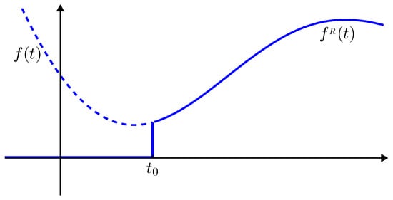
Figure 1. Replacement of $f\left(t\right)$ (dotted and solid lines) by $f^{\mathrm{R}}\left(t\right)$ (solid line) for a given point $t_0$.

It is quite intuitive to observe the following relationship between the GL derivative of $f^{\mathrm{R}}\left(t\right)$ and the truncated GL derivative (16) of the original function $f\left(t\right)$ and, in the end, of its RL derivative.

Proposition 4.

Let $\alpha >0$, $m=⌈\alpha ⌉$ and $f\in {\mathcal{C}}^m[t_0,T]$. Then, for any $t\in (t_0,T]$ it is:

$${}^{\mathit{GL}}{D}^{\alpha }{f}^R\left(t\right)={}^{\mathit{GL}}{D}_{t_0}^{\alpha }f\left(t\right)={}^{\mathit{RL}}{D}_{t_0}^{\alpha }f\left(t\right).$$

Proof. 

The application of the GL fractional derivative ${}^{\mathrm{GL}}{D}^{\alpha }$ to $f^{\mathrm{R}}\left(t\right)$ leads to:

$${}^{\mathrm{GL}}{D}^{\alpha }{f}^{\mathrm{R}}\left(t\right)=\underset{h\to 0}{lim}\frac{1}{h^{\alpha }}\sum _{j=0}^{\infty }{(-1)}^j\left(\genfrac{}{}{0pt}{}{\alpha }{j}\right)f^{\mathrm{R}}(t-jh)=\underset{h\to 0}{lim}\frac{1}{h^{\alpha }}\sum _{j=0}^N{(-1)}^j\left(\genfrac{}{}{0pt}{}{\alpha }{j}\right)f(t-jh)$$

where $N=⌈(t-t_0)/h⌉$ is the smallest integer such that $f^{\mathrm{R}}(t-jh)\equiv 0$ for $j=N+1,N+2,\dots$ and hence ${}^{\mathrm{GL}}{D}^{\alpha }{f}^{\mathrm{R}}\left(t\right)={}^{\mathrm{GL}}{D}_{t_0}^{\alpha }f\left(t\right)$. The second equality comes from (17). □

Unless $f\left(t_0\right)=0$, the replacement of $f\left(t\right)$ with $f^{\mathrm{R}}\left(t\right)$ introduces a discontinuity at $t_0$ and, even when $f\left(t_0\right)=0$, the function $f^{\mathrm{R}}\left(t\right)$ may suffer from a lack of regularity at $t_0$ due to the discontinuity of its higher-order derivatives. As we will see, this discontinuity seriously affects the RL derivative of several functions which, indeed, are often unbounded at $t_0$. Therefore, to provide a regularization and reduce the lack of smoothness introduced by $f^{\mathrm{R}}\left(t\right)$, a different replacement is proposed.

3.2. Replacement with a More Regular Function: The Caputo’s Derivative

An alternative approach is based on the replacement, as depicted in Figure 2, of $f\left(t\right)$ with a function having a more regular behavior at $t_0$, and whose regularity depends on $\alpha$. The proposed function is a continuation of $f\left(t\right)$ before $t_0$ in terms of its Taylor polynomial at $t_0$, namely:

$$f^{\mathrm{C}}\left(t\right)=\left\{\begin{array}{cc}{T}_{m-1}[f;t_0]\left(t\right)\hfill & t\in (-\infty ,t_0)\hfill \\ f\left(t\right)\hfill & t\ge t_0\hfill \end{array}\right.$$

where $T_{m-1}[f;t_0]\left(t\right)$ is the same Taylor polynomial of f centered at $t_0$ introduced in (8) and $m=⌈\alpha ⌉$. It is clear that, unlike $f^{\mathrm{R}}\left(t\right)$, the function $f^{\mathrm{C}}\left(t\right)$ preserves a possible smoothness of $f\left(t\right)$ at $t_0$ since:

$$f^{\mathrm{C}}\left(t\right){|}_{t\to t_0^{-}}=f\left(t_0\right),\frac{\mathrm{d}}{\mathrm{d}t}{f}^{\mathrm{C}}\left(t\right){|}_{t\to t_0^{-}}=f^{\prime }\left(t_0\right),\dots ,\frac{{\mathrm{d}}^{m-1}}{\mathrm{d}{t}^{m-1}}{f}^{\mathrm{C}}\left(t\right){|}_{t\to t_0^{-}}=f^{(m-1)}\left(t_0\right).$$

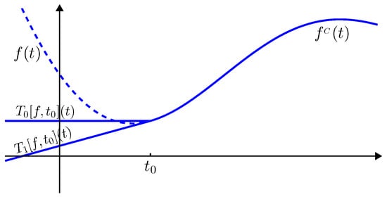
Figure 2. Replacement of $f\left(t\right)$ (dotted and solid lines) by $f^{\mathrm{C}}\left(t\right)$ (solid line) for a given point $t_0$ and for $m=0$ (branch labeled $T_0[f,t_0]\left(t\right)$) and $m=1$ (branch labeled $T_1[f,t_0]\left(t\right)$).

Before showing the effects of the replacement of $f\left(t\right)$ by $f^{\mathrm{C}}\left(t\right)$ we first have to consider the following preliminary result.

Lemma 1.

Let $\alpha >0$ and $m=⌈\alpha ⌉$. For any integer $k=0,1,\dots ,m-1$ it is:

$$\sum _{j=0}^{\infty }(-1)\left(\genfrac{}{}{0pt}{}{\alpha }{j}\right)j^k=0.$$

Proof. 

When $\alpha \in \mathbb{N}$ we refer to [26] (Proposition 2.1). Assume now $\alpha \notin \mathbb{N}$ and, after using the alternative formulation of the binomial coefficients, one obtains:

$$\sum _{j=0}^{\infty }(-1)\left(\genfrac{}{}{0pt}{}{\alpha }{j}\right)j^k=\frac{1}{\Gamma (-\alpha )}\sum _{j=0}^{\infty }\frac{\Gamma (j-\alpha )}{\Gamma (j+1)}{j}^k.$$

From [26] (Theorem 3.2) we know that the following asymptotic expansion holds:

$$\sum _{j=0}^n\frac{\Gamma (j-\alpha )}{\Gamma (j+1)}{j}^k=\sum _{\ell =0}^{\infty }{F}_{\ell }{n}^{k-\alpha -\ell },n\to \infty ,$$

with coefficients $F_{\ell }$ depending on $\alpha$ and k but not on n. The proof hence immediately follows since $k-\alpha <0$. □

We are now able to study the relationship between the GL derivative of $f^{\mathrm{C}}\left(t\right)$ and the truncated GL derivative (16) and the Caputo’s derivative (6) of $f\left(t\right)$.

Proposition 5.

Let $\alpha >0$, $m=⌈\alpha ⌉$ and $f\in {\mathcal{C}}^m[t_0,T]$. Then, for any $t\in (t_0,T]$ it is:

$${}^{\mathit{GL}}{D}^{\alpha }{f}^{\mathrm{C}}\left(t\right)={}^{\mathit{GL}}{D}_{t_0}^{\alpha }\left(f\left(t\right)-T_{m-1}[f;t_0]\left(t\right)\right)={}^C{D}_{t_0}^{\alpha }f\left(t\right).$$

Proof. 

The application of the GL fractional derivative ${}^{\mathrm{GL}}{D}^{\alpha }$ to $f^{\mathrm{C}}\left(t\right)$ leads to:

$$\begin{array}{cc}\hfill {}^{\mathrm{GL}}{D}^{\alpha }{f}^{\mathrm{C}}\left(t\right)& =\underset{h\to 0}{lim}\frac{1}{h^{\alpha }}\sum _{j=0}^{\infty }{(-1)}^j\left(\genfrac{}{}{0pt}{}{\alpha }{j}\right)f^{\mathrm{C}}(t-jh)\hfill \\ & =\underset{h\to 0}{lim}\frac{1}{h^{\alpha }}\left[\sum _{j=0}^N{(-1)}^j\left(\genfrac{}{}{0pt}{}{\alpha }{j}\right)f(t-jh)+\sum _{j=N+1}^{\infty }{(-1)}^j\left(\genfrac{}{}{0pt}{}{\alpha }{j}\right)T_{m-1}[f;t_0](t-jh)\right]\hfill \end{array}$$

Observe now that:

$$T_{m-1}[f;t_0](t-jh)=\sum _{k=0}^{m-1}\frac{{(t-jh-t_0)}^k}{k!}{f}^{\left(k\right)}\left(t_0\right)=\sum _{k=0}^{m-1}\frac{1}{k!}{f}^{\left(k\right)}\left(t_0\right)\sum _{\ell =0}^k\left(\genfrac{}{}{0pt}{}{k}{\ell }\right){(t-t_0)}^{\ell }{(-jh)}^{k-\ell }$$

and hence,

$$\sum _{j=N+1}^{\infty }{(-1)}^j\left(\genfrac{}{}{0pt}{}{\alpha }{j}\right)T_{m-1}[f;t_0](t-jh)=\sum _{k=0}^{m-1}\frac{1}{k!}{f}^{\left(k\right)}\left(t_0\right)\sum _{\ell =0}^k\left(\genfrac{}{}{0pt}{}{k}{\ell }\right){(-h)}^{k-\ell }{(t-t_0)}^{\ell }\sum _{j=N+1}^{\infty }{(-1)}^j\left(\genfrac{}{}{0pt}{}{\alpha }{j}\right)j^{k-\ell }.$$

Since from Lemma 1 it is:

$$\sum _{j=N+1}^{\infty }{(-1)}^j\left(\genfrac{}{}{0pt}{}{\alpha }{j}\right)j^k=-\sum _{j=0}^N{(-1)}^j\left(\genfrac{}{}{0pt}{}{\alpha }{j}\right)j^k$$

we obtain,

$$\begin{array}{cc}\hfill \sum _{j=N+1}^{\infty }{(-1)}^j& \left(\genfrac{}{}{0pt}{}{\alpha }{j}\right)T_{m-1}[f;t_0](t-jh)=-\sum _{k=0}^{m-1}\frac{1}{k!}{f}^{\left(k\right)}\left(t_0\right)\sum _{\ell =0}^k\left(\genfrac{}{}{0pt}{}{k}{\ell }\right){(-h)}^{k-\ell }{(t-t_0)}^{\ell }\sum _{j=0}^N{(-1)}^j\left(\genfrac{}{}{0pt}{}{\alpha }{j}\right)j^{k-\ell }\hfill \\ & =-\sum _{j=0}^N{(-1)}^j\left(\genfrac{}{}{0pt}{}{\alpha }{j}\right)\sum _{k=0}^{m-1}\frac{1}{k!}{f}^{\left(k\right)}\left(t_0\right)\sum _{\ell =0}^k\left(\genfrac{}{}{0pt}{}{k}{\ell }\right){(-hj)}^{k-\ell }{(t-t_0)}^{\ell }\hfill \\ & =-\sum _{j=0}^N{(-1)}^j\left(\genfrac{}{}{0pt}{}{\alpha }{j}\right)T_{m-1}[f;t_0](t-jh)\hfill \end{array}$$

from which the first equality follows. The second equality is consequence of Proposition 4 together with Equation (9). □

4. The Mittag–Leffler Function

The Mittag–Leffler (ML) function plays a special role in fractional calculus and in the representation of fractional derivatives of elementary functions and will be better investigated later on. It is therefore mandatory to recall some of the main properties of this function.

The definition of the two-parameter ML function is given by:

$$E_{\alpha ,\beta }\left(z\right)=\sum _{k=0}^{\infty }\frac{z^k}{\Gamma (\alpha k+\beta )},z\in \mathbb{C},$$

(18)

where $\alpha$ and $\beta$ are two (possibly complex, but with $Re\alpha >0$) parameters.

The importance of the ML function in fractional calculus is particularly related to the fact that it is the eigenfunction of RL and Caputo’s fractional derivatives. It is indeed possible to show that for any $t>t_0$ and $j=0,1,\cdots ,m-1$, with $m=⌈\alpha ⌉$, it is:

$$\begin{array}{cc}\hfill {}^{\mathrm{RL}}{D}_{t_0}^{\alpha }y\left(t\right)& =\Omega y\left(t\right),y\left(t\right)={(t-t_0)}^{\alpha -j-1}{E}_{\alpha ,\alpha -j}\left(\Omega {(t-t_0)}^{\alpha }\right),\hfill \\ \hfill {}^{\mathrm{C}}{D}_{t_0}^{\alpha }y\left(t\right)& =\Omega y\left(t\right),y\left(t\right)={(t-t_0)}^j{E}_{\alpha ,j+1}\left(\Omega {(t-t_0)}^{\alpha }\right),\hfill \end{array}$$

and therefore the ML function has in fractional calculus the same importance as the exponential in the integer-order calculus (indeed, the ML function generalizes the exponential since $E_{1,1}\left(z\right)={\mathrm{e}}^z$).

It is useful to introduce the Laplace transform (LT) of the ML function which, for any real $t>0$ and $z\in \mathbb{C}$, is given by:

$$\mathcal{L}\left(t^{\beta -1}{E}_{\alpha ,\beta }\left(t^{\alpha }z\right);s\right)=\frac{s^{\alpha -\beta }}{s^{\alpha }-z},Res>0,\left|z{s}^{-\alpha }\right|<1,$$

(19)

and, for convenience, we impose a branch cut on the negative real semi-axis in order to make the function $s^{\alpha }$ single valued.

The special instance $E_{1,\beta }\left(z\right)$ of the ML function will be encountered in the representation of fractional integrals and derivatives of some elementary functions. $E_{1,\beta }\left(z\right)$ is closely related to the exponential function and, as for instance emphasized in [27], it is:

$$E_{1,\beta }\left(z\right)={\mathrm{e}}^z·{\widehat{P}}_{\beta }\left(z\right),{\widehat{P}}_{\beta }\left(z\right)=\frac{1}{\Gamma (\beta -1)}\sum _{k=0}^{\infty }\frac{{(-z)}^k}{k!(\beta -1+k)}.$$

It is however more convenient to express the ML function as a deviation from the exponential function according to the following result which will turn out to be useful in the subsequent sections.

Theorem 1.

Let $\Omega \in \mathbb{C}$ with $|arg(\Omega \left)\right|<\pi$. For any $\beta >-1$ and $t\ge 0$ it is:

$$t^{-\beta }{E}_{1,1-\beta }(\Omega t)={\Omega }^{\beta }{\mathrm{e}}^{t\Omega }+F_{\beta }(t;\Omega ),$$

(20)

where,

$$F_{\beta }(t;\Omega )=\frac{sin\left(\beta \pi \right)}{\pi }{\int }_0^{\infty }{\mathrm{e}}^{-rt}\frac{r^{\beta }}{r+\Omega }\mathrm{d}r.$$

(21)

Proof. 

Thanks to Formula (19) for the LT of the ML we observe that:

$$\mathcal{L}\left(t^{-\beta }{E}_{1,1-\beta }(\Omega t);s\right)=\frac{s^{\beta }}{s-\Omega };$$

thus, the formula for the inversion of the LT allows to write this function as:

$$t^{-\beta }{E}_{1,1-\beta }(\Omega t)=\frac{1}{2\pi \mathrm{i}}{\int }_{\sigma -\mathrm{i}\infty }^{\sigma +\mathrm{i}\infty }{\mathrm{e}}^{st}\frac{s^{\beta }}{s-\Omega }\mathrm{d}s,\sigma >max\{0,Re\Omega \}.$$

The Bromwich line $(\sigma -\mathrm{i}\infty ,\sigma +\mathrm{i}\infty )$ can be deformed into an Hankel contour ${\mathcal{H}}_{ϵ}$ starting at $-\infty$ below the negative real semi-axis and ending at $-\infty$ above the negative real semi-axis after surrounding the origin along a circular disc $\left|s\right|=ϵ$. Since $\Omega$ does not lie on the branch cut, the contour ${\mathcal{H}}_{ϵ}$ can be collapsed onto the branch-cut by letting $ϵ\to 0$. The contour thus passes over the singularity $\Omega$ and the residue subtraction leads to:

$$t^{-\beta }{E}_{1,1-\beta }(\Omega t)=Res\left(e^{st}\frac{s^{\beta }}{s-\Omega },\Omega \right)+F_{\beta }(t;\Omega )$$

where, for shortness, we denoted:

$$F_{\beta }(t;\Omega )=\underset{ϵ\to 0}{lim}\frac{1}{2\pi \mathrm{i}}{\int }_{{\mathcal{H}}_{ϵ}}{\mathrm{e}}^{st}\frac{s^{\beta }}{s-\Omega }\mathrm{d}s.$$

The residue can be easily computed as:

$$Res\left(e^{st}\frac{s^{\beta }}{s-\Omega },\Omega \right)={\Omega }^{\beta }{\mathrm{e}}^{\Omega t},$$

whilst to evaluate $F_{\beta }(t;\Omega )$ we first decompose the Hankel contour into its three main paths:

$${\mathcal{H}}_{ϵ}={\gamma }_1+{\gamma }_2+{\gamma }_3,\left\{\begin{array}{cc}{\gamma }_1:s=r{\mathrm{e}}^{-\mathrm{i}\pi },\hfill & \infty >r\ge ϵ,\hfill \\ {\gamma }_2:s=ϵ{\mathrm{e}}^{\mathrm{i}\theta },\hfill & -\pi <\theta <\pi ,\hfill \\ {\gamma }_3:s=r{\mathrm{e}}^{\mathrm{i}\pi },\hfill & ϵ\le r<\infty ,\hfill \end{array}\right.$$

thanks to which we are able to write:

$$\frac{1}{2\pi \mathrm{i}}{\int }_{{\mathcal{H}}_{ϵ}}{\mathrm{e}}^{st}\frac{s^{\beta }}{s-\Omega }\mathrm{d}s=I_1+I_2+I_3,I_{\ell }=\frac{1}{2\pi \mathrm{i}}{\int }_{{\gamma }_{\ell }}{\mathrm{e}}^{st}\frac{s^{\beta }}{s-\Omega }\mathrm{d}s,\ell =1,2,3.$$

Since ${\mathrm{e}}^{\mathrm{i}\pi }={\mathrm{e}}^{-\mathrm{i}\pi }=-1$, it is possible to compute:

$$\begin{array}{cc}\hfill I_1& =\frac{1}{2\pi \mathrm{i}}{\int }_{\infty }^{ϵ}{\mathrm{e}}^{-rt}\frac{r^{\beta }{\mathrm{e}}^{-\mathrm{i}\beta \pi }{\mathrm{e}}^{-\mathrm{i}\pi }}{-r-\Omega }\mathrm{d}r=-\frac{{\mathrm{e}}^{-\mathrm{i}\beta \pi }}{2\pi \mathrm{i}}{\int }_{ϵ}^{\infty }{\mathrm{e}}^{-rt}\frac{r^{\beta }}{r+\Omega }\mathrm{d}r\hfill \\ \hfill I_2& =\frac{{ϵ}^{\beta +1}}{2\pi }{\int }_{-\pi }^{\pi }\frac{{\mathrm{e}}^{ϵtcos\theta +\mathrm{i}\left[\right(\beta +1)\theta +ϵtsin\theta ]}}{ϵcos\theta -\Omega +\mathrm{i}ϵsin\theta }\mathrm{d}\theta \hfill \\ \hfill I_3& =\frac{1}{2\pi \mathrm{i}}{\int }_{ϵ}^{\infty }{\mathrm{e}}^{-rt}\frac{r^{\beta }{\mathrm{e}}^{\mathrm{i}\beta \pi }{\mathrm{e}}^{\mathrm{i}\pi }}{-r-\Omega }\mathrm{d}r=\frac{{\mathrm{e}}^{\mathrm{i}\beta \pi }}{2\pi \mathrm{i}}{\int }_{ϵ}^{\infty }{\mathrm{e}}^{-rt}\frac{r^{\beta }}{r+\Omega }\mathrm{d}r\hfill \end{array}$$

and we observe that, due to the presence of the term ${ϵ}^{\beta +1}$, where we assumed $\beta >-1$, the integral $I_2$ vanishes when $ϵ\to 0$. For the remaining term $I_1+I_2$ we note that:

$$\frac{{\mathrm{e}}^{\mathrm{i}\beta \pi }}{2\pi \mathrm{i}}-\frac{{\mathrm{e}}^{-\mathrm{i}\beta \pi }}{2\pi \mathrm{i}}=\frac{sin\beta \pi }{\pi },$$

and, hence, the representation (21) of $F_{\beta }(t;\Omega )$ easily follows. □

The relationship between the ML function and the exponential is even more clear in the presence of an integer second parameter.

Proposition 6.

Let $m\in \mathbb{N}$ and $\Omega \in \mathbb{C}$. For any $t\in \mathbb{R}$ it is:

$$\begin{array}{c}{t}^m{E}_{1,1+m}(\Omega t)=\frac{1}{{\Omega }^m}\left({\mathrm{e}}^{\Omega t}-\sum _{j=0}^{m-1}\frac{{\Omega }^j{t}^j}{j!}\right),\hfill \\ t^{-m}{E}_{1,1-m}(\Omega t)={\Omega }^m{\mathrm{e}}^{\Omega t}.\hfill \end{array}$$

Proof. 

The first equality directly follows from the definition (18) of the ML function since it is:

$$t^m{E}_{1,1+m}(\Omega t)=\frac{1}{{\Omega }^m}\sum _{k=0}^{\infty }\frac{{\Omega }^{k+m}{t}^{k+m}}{\Gamma (k+1+m)}=\frac{1}{{\Omega }^m}\sum _{j=m}^{\infty }\frac{{\Omega }^j{t}^j}{\Gamma (j+1)}=\frac{1}{{\Omega }^m}\left(\sum _{j=0}^{\infty }\frac{{\Omega }^j{t}^j}{j!}-\sum _{j=0}^{m-1}\frac{{\Omega }^j{t}^j}{j!}\right)$$

whilst the second equality is a special case of Theorem 1. □

The following result will prove its particular utility when studying the asymptotic behavior of the fractional derivatives of some functions which will be expressed, in the next sections, in terms of special instances of the ML function.

Proposition 7.

Let $\beta >-1$, $\Omega \in \mathbb{C}$, $|arg\Omega |<\pi$, and $t\ge 0$. Then,

$$F_{\beta }(t;\Omega )=C_{\beta }{\Omega }^{-1}{t}^{-\beta -1}\left(1+\mathcal{O}\left(t^{-1}\right)\right),t\to \infty ,$$

with $C_{\beta }$ independent of t and Ω.

Proof. 

By a change of the integration variable we can write:

$$F_{\beta }(t;\Omega )={\Omega }^{\beta }\frac{sin\beta \pi }{\pi }{\int }_0^{\infty }{\mathrm{e}}^{-r\Omega t}\frac{r^{\beta }}{r+1}\mathrm{d}r={\Omega }^{\beta }\frac{sin\beta \pi }{\pi }\Gamma (\beta +1)U(\beta +1,\beta +1,\Omega t)$$

where $U(a,b,z)$ is the Tricomi function (often known as the confluent hypergeometric function of the second kind) defined for $Rea>0$ and $Rez>0$ and by analytic continuation elsewhere [28] (Chapter 48). After putting $C_{\beta }=\Gamma (\beta +1)sin\left(\beta \pi \right)/\pi$, it is therefore [29] (Chapter 7, § 10.1),

$$F_{\beta }(t;\Omega )\sim t^{-\beta -1}{C}_{\beta }{\Omega }^{-1}\sum _{j=0}^{\infty }{(-1)}^j\frac{\Gamma (\beta +1+j)}{\Gamma (\beta +1)}{t}^{-j}{\Omega }^{-j},t\to \infty ,|arg\Omega |\le \frac{3}{2}\pi -\delta$$

for arbitrary small $\delta >0$. Hence the proof follows since the selection of the branch cut on the negative real semi-axis. □

5. Fractional Integral and Derivatives of the Power Function

Basic results on fractional integral and derivatives of the power function ${(t-t_0)}^{\beta }$, for $\beta >-1$, are available in the literature; see, for instance [9] for the RL integral:

$$J_{t_0}^{\alpha }{(t-t_0)}^{\beta }=\frac{\Gamma (\beta +1)}{\Gamma (\beta +\alpha +1)}{(t-t_0)}^{\beta +\alpha },$$

(22)

for the RL derivative (as usual, $m=⌈\alpha ⌉$):

$${}^{\mathrm{RL}}{D}_{t_0}^{\alpha }{(t-t_0)}^{\beta }=\left\{\begin{array}{cc}0\hfill & \beta \in \left\{\alpha -m,\alpha -m+1,\dots ,\alpha -1\right\}\hfill \\ {\displaystyle \frac{\Gamma (\beta +1)}{\Gamma (\beta -\alpha +1)}{(t-t_0)}^{\beta -\alpha }}\hfill & \mathrm{otherwise}\hfill \end{array}\right.$$

(23)

and for the Caputo’s derivative:

$${}^{\mathrm{C}}{D}_{t_0}^{\alpha }{(t-t_0)}^{\beta }=\left\{\begin{array}{cc}0\hfill & \beta \in \left\{0,1,\dots ,m-1\right\}\hfill \\ {\displaystyle \frac{\Gamma (\beta +1)}{\Gamma (\beta -\alpha +1)}{(t-t_0)}^{\beta -\alpha }}\hfill & \beta >m-1\hfill \\ \mathrm{non}\mathrm{existing}\hfill & \mathrm{otherwise}\hfill \end{array}\right.$$

(24)

The absence of the Caputo’s derivative of ${(t-t_0)}^{\beta }$ for real $\beta <m-1$ with $\beta \notin \left\{0,1,\dots ,m-1\right\}$ is related to the fact that once the m-th order derivative of ${(t-t_0)}^{\beta }$ is evaluated the integrand in Equation (6) is no longer integrable.

For general power functions independent from the starting point, i.e., for $t^k$ instead of ${(t-t_0)}^k$, we can provide the following results.

Proposition 8.

Let $\alpha >0$ and $m=⌈\alpha ⌉$. Then for any $k\in \mathbb{N}$:

1.

${}^{\mathit{GL}}{D}^{\alpha }{t}^k=0$ for $k<\alpha$;

2.

${\displaystyle {}^{\mathit{RL}}{D}_{t_0}^{\alpha }{t}^k=\sum _{\ell =0}^k\frac{k!}{(k-\ell )!\Gamma (\ell +1-\alpha )}{(t-t_0)}^{\ell -\alpha }{t}_0^{k-\ell }}$;

3.

${}^C{D}_{t_0}^{\alpha }{t}^k=\left\{\begin{array}{cc}0\hfill & ifk<\alpha \hfill \\ {\displaystyle \sum _{\ell =m}^k\frac{k!}{(k-\ell )!\Gamma (\ell +1-\alpha )}{(t-t_0)}^{\ell -\alpha }{t}_0^{k-\ell }}\hfill & \mathit{otherwhise}\hfill \end{array}\right.$

Proof. 

For ${}^{\mathrm{GL}}{D}^{\alpha }{t}^k$ we first write:

$${(t-jh)}^k=\sum _{\ell =0}^k\left(\genfrac{}{}{0pt}{}{k}{\ell }\right)t^{\ell }{(-h)}^{k-\ell }{j}^{k-\ell }$$

and hence by using the Definition 4 it is possible to see that:

$${}^{\mathrm{GL}}{D}^{\alpha }{t}^k=\underset{h\to 0}{lim}\frac{1}{h^{\alpha }}\sum _{j=0}^{\infty }{(-1)}^j\left(\genfrac{}{}{0pt}{}{\alpha }{j}\right){(t-jh)}^k=\underset{h\to 0}{lim}\frac{1}{h^{\alpha }}\sum _{\ell =0}^k\left(\genfrac{}{}{0pt}{}{k}{\ell }\right)t^{\ell }{(-h)}^{k-\ell }\sum _{j=0}^{\infty }{(-1)}^j\left(\genfrac{}{}{0pt}{}{\alpha }{j}\right)j^{k-\ell }=0$$

where we applied Lemma 1. For ${}^{\mathrm{RL}}{D}_{t_0}^{\alpha }{t}^k$ we expand:

$$t^k=\sum _{\ell =0}^k\left(\genfrac{}{}{0pt}{}{k}{\ell }\right){(t-t_0)}^{\ell }{t}_0^{k-\ell }$$

and hence the proof immediately follows from Equation (23). Similarly for ${}^{\mathrm{C}}{D}_{t_0}^{\alpha }{t}^k$ by using Equation (24). □

Note that ${}^{\mathrm{GL}}{D}^{\alpha }{t}^k$ diverges when $k>\alpha$. A representation of ${}^{\mathrm{C}}{D}_{t_0}^{\alpha }{t}^{\beta }$, for general real but not integer $\beta$, is provided in terms of the hypergeometric ${}_2{F}_1$ function in [9] (Appendix B).

6. Fractional Integral and Derivatives of the Exponential Function

The exponential function is of great importance in mathematics and in several applications, also to approximate other functions. We therefore study here fractional integral and derivatives of the exponential function.

Proposition 9.

Let $\alpha >0$, $m=\lceil \alpha \rceil$ and $t_0\in \mathbb{R}$. For any $\Omega \in \mathbb{C}$ and $t>t_0$ the exponential function ${\mathrm{e}}^{\Omega (t-t_0)}$ has the following fractional integral and derivatives:

$$\begin{array}{c}{J}_{t_0}^{\alpha }{\mathrm{e}}^{\Omega (t-t_0)}={(t-t_0)}^{\alpha }{E}_{1,1+\alpha }(\Omega (t-t_0)),\hfill \\ {}^{RL}{D}_{t_0}^{\alpha }{\mathrm{e}}^{\Omega (t-t_0)}={(t-t_0)}^{-\alpha }{E}_{1,1-\alpha }(\Omega (t-t_0)),\hfill \\ {}^C{D}_{t_0}^{\alpha }{\mathrm{e}}^{\Omega (t-t_0)}={\Omega }^m{(t-t_0)}^{m-\alpha }{E}_{1,m-\alpha +1}(\Omega (t-t_0)),\hfill \end{array}$$

and, moreover, for any $t\in \mathbb{R}$ and $Re(\Omega )\ge 0$ it is:

$$\begin{array}{cc}{}^{GL}{D}^{\alpha }{\mathrm{e}}^{\Omega t}={\Omega }^{\alpha }{\mathrm{e}}^{\Omega t}.\hfill & \phantom{}\hfill \end{array}$$

Proof. 

By applying a term-by-term integration to the series expansion of the exponential function:

$${\mathrm{e}}^{\Omega t}=\sum _{k=0}^{\infty }\frac{{\Omega }^k{t}^k}{k!},$$

(25)

and thanks to Equation (22) and to Definition (18) of the ML function, we obtain:

$$J_{t_0}^{\alpha }{\mathrm{e}}^{\Omega (t-t_0)}=\sum _{k=0}^{\infty }\frac{{\Omega }^k}{k!}{J}_{t_0}^{\alpha }{(t-t_0)}^k=\sum _{k=0}^{\infty }\frac{{\Omega }^k}{\Gamma (k+\alpha +1)}{(t-t_0)}^{k+\alpha }={(t-t_0)}^{\alpha }{E}_{1,1+\alpha }(\Omega (t-t_0)).$$

For the evaluation of the RL derivative ${}^{\mathrm{RL}}{D}_0^{\alpha }{\mathrm{e}}^{\Omega (t-t_0)}$ we again consider the series expansion Equation (25) and, by differentiating term by term thanks to Equation (23), it is:

$${}^{\mathrm{RL}}{D}_{t_0}^{\alpha }{\mathrm{e}}^{\Omega (t-t_0)}={}^{\mathrm{RL}}{D}_{t_0}^{\alpha }\sum _{k=0}^{\infty }\frac{{\Omega }^k{(t-t_0)}^k}{k!}=\sum _{k=0}^{\infty }\frac{{\Omega }^k}{k!}{}^{\mathrm{RL}}{D}_{t_0}^{\alpha }{(t-t_0)}^k=\sum _{k=0}^{\infty }\frac{{\Omega }^k{(t-t_0)}^{k-\alpha }}{\Gamma (k-\alpha +1)}$$

from which the proof follows thanks again to Definition (18) of the ML function. We proceed in a similar way for ${}^{\mathrm{C}}{D}_{t_0}^{\alpha }{\mathrm{e}}^{\Omega (t-t_0)}$ for which it is:

$${}^{\mathrm{C}}{D}_{t_0}^{\alpha }{\mathrm{e}}^{\Omega (t-t_0)}={}^{\mathrm{C}}{D}_{t_0}^{\alpha }\left(\sum _{k=0}^{m-1}\frac{{\Omega }^k{(t-t_0)}^k}{k!}+\sum _{k=m}^{\infty }\frac{{\Omega }^k{(t-t_0)}^k}{k!}\right)=\sum _{k=m}^{\infty }\frac{{\Omega }^k}{k!}{}^{\mathrm{C}}{D}_{t_0}^{\alpha }{(t-t_0)}^k=\sum _{k=m}^{\infty }\frac{{\Omega }^k{(t-t_0)}^{k-\alpha }}{\Gamma (k-\alpha +1)}$$

and, after a change $j=k-m$ in the summation index and rearranging some terms we obtain:

$${}^{\mathrm{C}}{D}_{t_0}^{\alpha }{\mathrm{e}}^{\Omega (t-t_0)}=\sum _{j=0}^{\infty }\frac{{\Omega }^{j+m}{(t-t_0)}^{j+m-\alpha }}{\Gamma (j+m-\alpha +1)}={\Omega }^m{(t-t_0)}^{m-\alpha }\sum _{j=0}^{\infty }\frac{{\Omega }^j{(t-t_0)}^j}{\Gamma (j+m-\alpha +1)}$$

from which, again, the proof follows from Definition (18) of the ML function. To finally evaluate the GL derivative ${}^{\mathrm{GL}}{D}^{\alpha }{\mathrm{e}}^{\Omega t}$ we first apply its definition from Equation (15)

$${}^{\mathrm{GL}}{D}^{\alpha }{\mathrm{e}}^{\Omega t}=\underset{h\to 0}{lim}\frac{1}{h^{\alpha }}\sum _{j=0}^{\infty }{(-1)}^j\left(\genfrac{}{}{0pt}{}{\alpha }{j}\right){\mathrm{e}}^{\Omega (t-jh)}={\mathrm{e}}^{\Omega t}\underset{h\to 0}{lim}\frac{1}{h^{\alpha }}\sum _{j=0}^{\infty }{(-1)}^j\left(\genfrac{}{}{0pt}{}{\alpha }{j}\right){\mathrm{e}}^{-jh\Omega }$$

and, since we are assuming $Re(\Omega )\ge 0$, it is $|{\mathrm{e}}^{-h\Omega }|\le 1$ and hence the binomial series converges:

$$\sum _{j=0}^{\infty }{(-1)}^j\left(\genfrac{}{}{0pt}{}{\alpha }{j}\right){\mathrm{e}}^{-jh\Omega }={\left(1-{\mathrm{e}}^{-h\Omega }\right)}^{\alpha }$$

(26)

thanks to which we can easily evaluate:

$${}^{\mathrm{GL}}{D}^{\alpha }{\mathrm{e}}^{\Omega t}={\mathrm{e}}^{\Omega t}\underset{h\to 0}{lim}\frac{{(1-{\mathrm{e}}^{-h\Omega })}^{\alpha }}{h^{\alpha }}={\mathrm{e}}^{\Omega t}\underset{h\to 0}{lim}{\left(\frac{1-{\mathrm{e}}^{-h\Omega }}{h}\right)}^{\alpha }={\Omega }^{\alpha }{\mathrm{e}}^{\Omega t}$$

to conclude the proof: □

Whenever $\alpha \in \mathbb{N}$, and hence $m=\alpha$, the standard integer-order results,

$$J_{t_0}^m{\mathrm{e}}^{\Omega (t-t_0)}=\frac{1}{{\Omega }^m}\left({\mathrm{e}}^{\Omega (t-t_0)}-\sum _{j=0}^{m-1}\frac{{(t-t_0)}^j}{j!}\right),D^m{\mathrm{e}}^{\Omega (t-t_0)}={\Omega }^m{\mathrm{e}}^{\Omega (t-t_0)}$$

are recovered. This is a direct consequence of Proposition 6 for $J_{t_0}^{\alpha }$ and ${}^{\mathrm{RL}}{D}_{t_0}^{\alpha }$ whilst it comes from the equivalence ${\mathrm{e}}^z=E_{1,1}\left(z\right)$ for ${}^{\mathrm{C}}{D}_{t_0}^{\alpha }$. It is moreover obvious for ${}^{\mathrm{GL}}{D}^{\alpha }$, for which we just observed that the restriction $Re(\Omega )\ge 0$ is no longer necessary when $\alpha \in \mathbb{N}$ since the binomial series (26) has just a finite number of nonzero terms and hence converges for any $\Omega \in \mathbb{C}$.

The correspondence ${}^{\mathrm{GL}}{D}^{\alpha }{\mathrm{e}}^{\Omega t}={\Omega }^{\alpha }{\mathrm{e}}^{\Omega t}$ appears as the most natural generalization of the integer-order derivatives but it holds only when $Re(\Omega )\ge 0$. By combining Proposition 9 and Theorem 1 it is immediately seen that ${}^{\mathrm{RL}}{D}_{t_0}^{\alpha }{\mathrm{e}}^{\Omega (t-t_0)}$ and ${}^{\mathrm{C}}{D}_{t_0}^{\alpha }{\mathrm{e}}^{\Omega (t-t_0)}$ can be represented as a deviation from ${\Omega }^{\alpha }{\mathrm{e}}^{\Omega t}$ as stated in the following result.

Proposition 10.

Let $\alpha >0$, $m=\lceil \alpha \rceil$ and $t_0\in \mathbb{R}$. For any $\Omega \in \mathbb{C}$, $|arg\Omega |<\pi$, and $t>t_0$ it is:

$$\begin{array}{c}{}^{\mathit{RL}}{D}_{t_0}^{\alpha }{\mathrm{e}}^{\Omega (t-t_0)}={\Omega }^{\alpha }{\mathrm{e}}^{\Omega (t-t_0)}+F_{\alpha }(t-t_0;\Omega ),\hfill \\ {}^C{D}_{t_0}^{\alpha }{\mathrm{e}}^{\Omega (t-t_0)}={\Omega }^{\alpha }{\mathrm{e}}^{\Omega (t-t_0)}+{\Omega }^m{F}_{\alpha -m}(t-t_0;\Omega ).\hfill \end{array}$$

The terms $F_{\alpha }(t-t_0,\Omega )$ and ${\Omega }^m{F}_{\alpha -m}(t-t_0,\Omega )$ describe the deviation of ${}^{\mathrm{RL}}{D}_{t_0}^{\alpha }{\mathrm{e}}^{\Omega (t-t_0)}$ and ${}^{\mathrm{C}}{D}_{t_0}^{\alpha }{\mathrm{e}}^{\Omega (t-t_0)}$ from the ideal value ${\Omega }^{\alpha }{\mathrm{e}}^{\Omega (t-t_0)}$. From Proposition 7 we know that these deviations decrease in magnitude, until they vanish, as $t\to \infty$. Consequently, ${}^{\mathrm{RL}}{D}_{t_0}^{\alpha }{\mathrm{e}}^{\Omega (t-t_0)}$ and ${}^{\mathrm{C}}{D}_{t_0}^{\alpha }{\mathrm{e}}^{\Omega (t-t_0)}$ asymptotically tend to ${\Omega }^{\alpha }{\mathrm{e}}^{\Omega (t-t_0)}$ (and hence to ${}^{\mathrm{GL}}{D}^{\alpha }{\mathrm{e}}^{\Omega (t-t_0)}$ when $Re\Omega \ge 0$), namely:

$${}^{\mathrm{RL}}{D}_{t_0}^{\alpha }{\mathrm{e}}^{\Omega (t-t_0)}\sim {}^{\mathrm{C}}{D}_{t_0}^{\alpha }{\mathrm{e}}^{\Omega (t-t_0)}\sim {\Omega }^{\alpha }{\mathrm{e}}^{\Omega (t-t_0)},t\to \infty ,|arg\Omega |<\pi .$$

This asymptotic behavior can be explained by recalling that the above derivatives differ from the way in which the function is assumed before the starting point $t_0$ and the influence of the function on $(-\infty ,t_0)$ clearly becomes of less and less importance as t goes away from $t_0$, namely as $t\to \infty$.

We observe from Figure 3, where the values $\alpha =0.7$ and $\Omega =-0.5+2\mathrm{i}$ have been considered, that actually both ${}^{\mathrm{RL}}{D}_{t_0}^{\alpha }{\mathrm{e}}^{\Omega t}$ and ${}^{\mathrm{C}}{D}_{t_0}^{\alpha }{\mathrm{e}}^{\Omega t}$ converge towards ${\Omega }^{\alpha }{\mathrm{e}}^{\Omega t}$, in quite a fast way, as t increases. In all the experiments we used, for ease of presentation, $t_0=0$ and the ML function was evaluated by means of the Matlab code described in [30] and based on some ideas previously developed in [31].

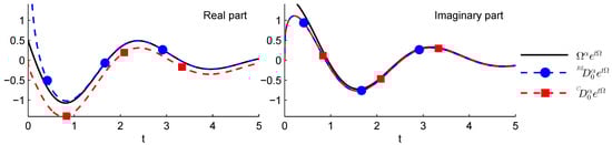
Figure 3. Comparison of ${}^{\mathrm{RL}}{D}_0^{\alpha }{\mathrm{e}}^{\Omega t}$ and ${}^{\mathrm{C}}{D}_0^{\alpha }{\mathrm{e}}^{\Omega t}$ with ${\Omega }^{\alpha }{\mathrm{e}}^{\Omega t}$ for $\alpha =0.7$ and $\Omega =-0.5+2\mathrm{i}$.

The unbounded nature of the real part of ${}^{\mathrm{RL}}{D}_{t_0}^{\alpha }{\mathrm{e}}^{\Omega t}$ at the origin is due to the presence of the factor ${(t-t_0)}^{-\alpha }$ (see Proposition 9) but it can also be interpreted as a consequence of the replacement of $f\left(t\right)$ by $f^{\mathrm{R}}\left(t\right)$ in the RL derivative, as discussed in Section 3.1, which introduces a discontinuity at the starting point; the same phenomena will be observed for the cosine function but, obviously, not for the sine function for which the value at 0 is the same forced in $(-\infty ,0)$.

It is not surprising that ${}^{\mathrm{RL}}{D}_{t_0}^{\alpha }{\mathrm{e}}^{\Omega t}$ and ${}^{\mathrm{C}}{D}_{t_0}^{\alpha }{\mathrm{e}}^{\Omega t}$ have the same imaginary part (which indeed overlap in the second plot of Figure 3) when $0<\alpha <1$. The imaginary part of the exponential is indeed zero at the origin and hence RL and Caputo’s derivatives coincide since relation in Equation (9) for $0<\alpha <1$ simply reads as ${}^{\mathrm{C}}{D}_{t_0}^{\alpha }f\left(t\right)={}^{\mathrm{RL}}{D}_{t_0}^{\alpha }\left(f\left(t\right)-f\left(t_0\right)\right)$.

From Figure 3 we observe that the RL derivative converges faster to ${\Omega }^{\alpha }{\mathrm{e}}^{\Omega t}$ than the Caputo derivative. This behavior can be easily explained by observing from Proposition 10 that as $t\to \infty$:

$$\begin{array}{c}{}^{\mathrm{RL}}{D}_{t_0}^{\alpha }{\mathrm{e}}^{\Omega (t-t_0)}-{\Omega }^{\alpha }{\mathrm{e}}^{\Omega (t-t_0)}=F_{\alpha }(t-t_0;\Omega )\sim {(t-t_0)}^{-\alpha -1}\hfill \\ {}^{\mathrm{C}}{D}_{t_0}^{\alpha }{\mathrm{e}}^{\Omega (t-t_0)}-{\Omega }^{\alpha }{\mathrm{e}}^{\Omega (t-t_0)}={\Omega }^m{F}_{\alpha -m}(t-t_0;\Omega )\sim {(t-t_0)}^{m-\alpha -1}\hfill \end{array}$$

which tell us that while ${}^{\mathrm{C}}{D}_{t_0}^{\alpha }{\mathrm{e}}^{\Omega (t-t_0)}$ converges towards ${\Omega }^{\alpha }{\mathrm{e}}^{\Omega (t-t_0)}$ according to a power law with exponent $-1<m-\alpha -1<0$, the RL derivative ${}^{\mathrm{RL}}{D}_{t_0}^{\alpha }{\mathrm{e}}^{\Omega (t-t_0)}$ converges according to a power law with exponent $-\alpha -1<-1$.

Similar behaviors, showing the convergence for $t\to \infty$ of the different derivatives, are obtained also for $\alpha =1.7$ and $\Omega =-0.5+2\mathrm{i}$ as we can observe from Figure 4. In this case, however, the imaginary parts of ${}^{\mathrm{RL}}{D}_{t_0}^{\alpha }{\mathrm{e}}^{\Omega t}$ and ${}^{\mathrm{C}}{D}_{t_0}^{\alpha }{\mathrm{e}}^{\Omega t}$ are no longer the same since when $1<\alpha <2$ the relationship between the two derivatives is given by ${}^{\mathrm{C}}{D}_{t_0}^{\alpha }f\left(t\right)={}^{\mathrm{RL}}{D}_{t_0}^{\alpha }\left(f\left(t\right)-f\left(t_0\right)-(t-t_0)f^{\prime }\left(t_0\right)\right)$ and the imaginary part of $f^{\prime }\left(t_0\right)$ is not equal to 0 as the imaginary part of $f\left(t_0\right)$.

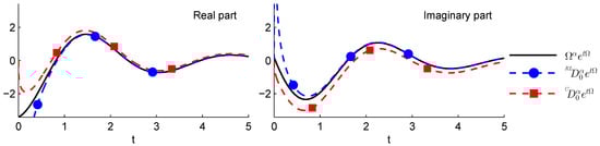
Figure 4. Comparison of ${}^{\mathrm{RL}}{D}_0^{\alpha }{\mathrm{e}}^{\Omega t}$ and ${}^{\mathrm{C}}{D}_0^{\alpha }{\mathrm{e}}^{\Omega t}$ with ${\Omega }^{\alpha }{\mathrm{e}}^{\Omega t}$ for $\alpha =1.7$ and $\Omega =-0.5+2\mathrm{i}$.

7. Fractional Integral and Derivatives of Sine and Cosine Functions

Once fractional derivatives of the exponential are available, the fractional derivatives of the basic trigonometric functions can be easily evaluated by means of the well-known De Moivre formulas:

$$sin\Omega t=\frac{{\mathrm{e}}^{\mathrm{i}\Omega t}-{\mathrm{e}}^{-\mathrm{i}\Omega t}}{2\mathrm{i}},cos\Omega t=\frac{{\mathrm{e}}^{\mathrm{i}\Omega t}+{\mathrm{e}}^{-\mathrm{i}\Omega t}}{2},$$

which allow to state the following results.

Proposition 11.

Let $\alpha >0$, $m=\lceil \alpha \rceil$ and $\Omega \in \mathbb{R}$. For $t\ge t_0$ the function $sin\left(\Omega (t-t_0)\right)$ has the following fractional integral and derivatives:

$$\begin{array}{c}{J}_{t_0}^{\alpha }sin\left(\Omega (t-t_0)\right)=\frac{{(t-t_0)}^{\alpha }}{2\mathrm{i}}\left(E_{1,1+\alpha }(+\mathrm{i}\Omega (t-t_0))-E_{1,1+\alpha }(-\mathrm{i}\Omega (t-t_0))\right)\hfill \\ {}^{\mathit{RL}}{D}_{t_0}^{\alpha }sin\left(\Omega (t-t_0)\right)=\frac{{(t-t_0)}^{-\alpha }}{2\mathrm{i}}\left(E_{1,1-\alpha }(+\mathrm{i}\Omega (t-t_0))-E_{1,1-\alpha }(-\mathrm{i}\Omega (t-t_0))\right)\hfill \\ {}^C{D}_{t_0}^{\alpha }sin\left(\Omega (t-t_0)\right)={\mathrm{i}}^m{\Omega }^m\frac{{(t-t_0)}^{m-\alpha }}{2\mathrm{i}}\left(E_{1,m-\alpha +1}(+\mathrm{i}\Omega (t-t_0))-{(-1)}^m{E}_{1,m-\alpha +1}(-\mathrm{i}\Omega (t-t_0))\right)\hfill \end{array}$$

and, moreover, for any $t\in \mathbb{R}$ it is:

$$\begin{array}{c}{}^{\mathit{GL}}{D}^{\alpha }sin\left(\Omega t\right)={\Omega }^{\alpha }sin\left(\Omega t+\alpha \frac{\pi }{2}\right).\hfill \end{array}$$

Proof. 

The proof for $J_{t_0}^{\alpha }sin\left(\Omega (t-t_0)\right)$, ${}^{\mathrm{RL}}{D}_{t_0}^{\alpha }sin\left(\Omega (t-t_0)\right)$ and ${}^{\mathrm{C}}{D}_{t_0}^{\alpha }sin\left(\Omega (t-t_0)\right)$ is a straightforward consequence of Proposition 9. For ${}^{\mathrm{GL}}{D}^{\alpha }sin\left(\Omega t\right)$ we observe that the direct application of Proposition 9 leads to:

$${}^{\mathrm{GL}}{D}^{\alpha }sin\left(\Omega t\right)=\frac{{(+\mathrm{i})}^{\alpha }{\Omega }^{\alpha }{\mathrm{e}}^{+\mathrm{i}\Omega t}-{(-\mathrm{i})}^{\alpha }{\Omega }^{\alpha }{\mathrm{e}}^{-\mathrm{i}\Omega t}}{2\mathrm{i}}$$

(27)

and since ${\mathrm{e}}^{\pm \mathrm{i}\Omega t}=cos\Omega t\pm \mathrm{i}sin\Omega t$ and ${(\pm \mathrm{i})}^{\alpha }={\mathrm{e}}^{\pm \mathrm{i}\alpha \pi /2}$, the proof follows from the application of basic trigonometric rules. □

Note that the assumption $Re\Omega \ge 0$ is no longer necessary for ${}^{\mathrm{GL}}{D}^{\alpha }sin\left(\Omega t\right)$ since the arguments of the exponential functions in Equation (27) are always on the imaginary axis. Similar results can also be stated for the cosine function and the proofs are omitted since they are similar to the previous ones.

Proposition 12.

Let $\alpha >0$, $m=\lceil \alpha \rceil$ and $\Omega \in \mathbb{R}$. For $t\ge t_0$ the function $cos\left(\Omega (t-t_0)\right)$ has the following fractional integral and derivatives:

$$\begin{array}{c}{J}_{t_0}^{\alpha }cos\left(\Omega (t-t_0)\right)=\frac{{(t-t_0)}^{\alpha }}{2}\left(E_{1,1+\alpha }(+\mathrm{i}\Omega (t-t_0))+E_{1,1+\alpha }(-\mathrm{i}\Omega (t-t_0))\right)\hfill \\ {}^{\mathit{RL}}{D}_{t_0}^{\alpha }cos\left(\Omega (t-t_0)\right)=\frac{{(t-t_0)}^{-\alpha }}{2}\left(E_{1,1-\alpha }(+\mathrm{i}\Omega (t-t_0))+E_{1,1-\alpha }(-\mathrm{i}\Omega (t-t_0))\right)\hfill \\ {}^C{D}_{t_0}^{\alpha }cos\left(\Omega (t-t_0)\right)={\mathrm{i}}^m{\Omega }^m\frac{{(t-t_0)}^{m-\alpha }}{2}\left(E_{1,m-\alpha +1}(+\mathrm{i}\Omega (t-t_0))+{(-1)}^m{E}_{1,m-\alpha +1}(-\mathrm{i}\Omega (t-t_0))\right)\hfill \end{array}$$

and, moreover, for any $t\in \mathbb{R}$ it is:

$$\begin{array}{c}{}^{\mathit{GL}}{D}^{\alpha }cos\left(\Omega t\right)={\Omega }^{\alpha }cos\left(\Omega t+\alpha \frac{\pi }{2}\right).\hfill \end{array}$$

As for the exponential function, we observe that with the basic trigonometric functions, the GL derivative ${}^{\mathrm{GL}}{D}^{\alpha }$ generalizes the known results holding for integer-order derivatives.

Furthermore, in this case, with the help of Proposition 1, it is possible to see that the RL and Caputo’s derivatives of $sin\left(\Omega (t-t_0)\right)$ and $cos\left(\Omega (t-t_0)\right)$ can be expressed as deviations from ${\Omega }^{\alpha }sin\left(\Omega t+\alpha \frac{\pi }{2}\right)$ and ${\Omega }^{\alpha }cos\left(\Omega t+\alpha \frac{\pi }{2}\right)$ respectively. The following results (whose proof is omitted since it is obvious) can indeed be provided.

Proposition 13.

Let $\alpha >0$, $m=\lceil \alpha \rceil$ and $\Omega \in \mathbb{R}$. Then for any $t\ge t_0$ it is:

$$\begin{array}{cc}\hfill {}^{\mathit{RL}}{D}_{t_0}^{\alpha }sin\left(\Omega (t-t_0)\right)& ={\Omega }^{\alpha }sin\left(\Omega (t-t_0)+\alpha \frac{\pi }{2}\right)+\frac{F_{\alpha }(t-t_0;\mathrm{i}\Omega )-F_{\alpha }(t-t_0;-\mathrm{i}\Omega )}{2\mathrm{i}}\hfill \\ \hfill {}^C{D}_{t_0}^{\alpha }sin\left(\Omega (t-t_0)\right)& ={\Omega }^{\alpha }sin\left(\Omega (t-t_0)+\alpha \frac{\pi }{2}\right)+{\mathrm{i}}^m{\Omega }^m\frac{F_{\alpha -m}(t-t_0;\mathrm{i}\Omega )-{(-1)}^m{F}_{\alpha -m}(t-t_0;-\mathrm{i}\Omega )}{2\mathrm{i}}\hfill \\ \hfill {}^{\mathit{RL}}{D}_{t_0}^{\alpha }cos\left(\Omega (t-t_0)\right)& ={\Omega }^{\alpha }cos\left(\Omega (t-t_0)+\alpha \frac{\pi }{2}\right)+\frac{F_{\alpha }(t-t_0;\mathrm{i}\Omega )+F_{\alpha }(t-t_0;-\mathrm{i}\Omega )}{2}\hfill \\ \hfill {}^C{D}_{t_0}^{\alpha }cos\left(\Omega (t-t_0)\right)& ={\Omega }^{\alpha }cos\left(\Omega (t-t_0)+\alpha \frac{\pi }{2}\right)+{\mathrm{i}}^m{\Omega }^m\frac{F_{\alpha -m}(t-t_0;\mathrm{i}\Omega )+{(-1)}^m{F}_{\alpha -m}(t-t_0;-\mathrm{i}\Omega )}{2}\hfill \end{array}$$

Since the function $F_{\beta }(t;\pm \mathrm{i}\Omega )$ asymptotically vanishes when $t\to \infty$, we can argue that:

$$\begin{array}{cc}\hfill {}^{\mathrm{RL}}{D}_{t_0}^{\alpha }sin\left(\Omega (t-t_0)\right)& \sim {}^{\mathrm{C}}{D}_{t_0}^{\alpha }sin\left(\Omega (t-t_0)\right)\sim {\Omega }^{\alpha }sin\left(\Omega t+\alpha \frac{\pi }{2}\right),t\to \infty \hfill \\ \hfill {}^{\mathrm{RL}}{D}_{t_0}^{\alpha }cos\left(\Omega (t-t_0)\right)& \sim {}^{\mathrm{C}}{D}_{t_0}^{\alpha }cos\left(\Omega (t-t_0)\right)\sim {\Omega }^{\alpha }cos\left(\Omega t+\alpha \frac{\pi }{2}\right),t\to \infty \hfill \end{array}$$

(28)

as we can clearly observe from Figure 5 and Figure 6.

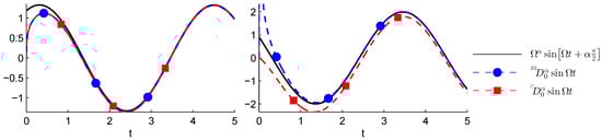
Figure 5. Comparison of ${}^{\mathrm{RL}}{D}_0^{\alpha }sin\Omega t$ and ${}^{\mathrm{C}}{D}_0^{\alpha }sin\Omega t$ with ${\Omega }^{\alpha }sin\left(\Omega t+\alpha \frac{\pi }{2}\right)$ for $\Omega =1.5$, $\alpha =0.7$ (left plot) and $\alpha =1.7$ (right plot).

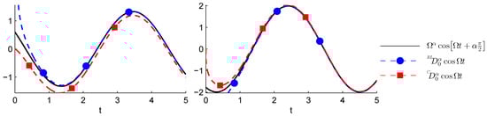
Figure 6. Comparison of ${}^{\mathrm{RL}}{D}_0^{\alpha }cos\Omega t$ and ${}^{\mathrm{C}}{D}_0^{\alpha }cos\Omega t$ with ${\Omega }^{\alpha }cos\left(\Omega t+\alpha \frac{\pi }{2}\right)$ for $\Omega =1.5$, $\alpha =0.7$ (left plot) and $\alpha =1.7$ (right plot).

The above results are mainly useful for studying the asymptotic behavior of different operators applied to the sine and cosine functions. The representation of integrals and derivatives can be simplified thanks to the following results.

Proposition 14.

Let $\alpha >0$, $m=\lceil \alpha \rceil$ and $\Omega \in \mathbb{R}$. For $t\ge t_0$ the function $sin\left(\Omega (t-t_0)\right)$ has the following fractional integral and derivatives:

$$\begin{array}{c}{J}_{t_0}^{\alpha }sin\left(\Omega (t-t_0)\right)=\Omega {(t-t_0)}^{1+\alpha }{E}_{2,2+\alpha }(-{\Omega }^2{(t-t_0)}^2)\hfill \\ {}^{\mathit{RL}}{D}_{t_0}^{\alpha }sin\left(\Omega (t-t_0)\right)=\Omega {(t-t_0)}^{1-\alpha }{E}_{2,2-\alpha }(-{\Omega }^2{(t-t_0)}^2)\hfill \\ {}^C{D}_{t_0}^{\alpha }sin\left(\Omega (t-t_0)\right)=\left\{\begin{array}{cc}{\displaystyle {(-1)}^{\frac{m-1}{2}}{\Omega }^m{(t-t_0)}^{m-\alpha }{E}_{2,m-\alpha +1}(-{\Omega }^2{(t-t_0)}^2)}\hfill & \mathit{odd}m\hfill \\ {\displaystyle {(-1)}^{\frac{m}{2}}{\Omega }^{m+1}{(t-t_0)}^{m-\alpha +1}{E}_{2,m-\alpha +2}(-{\Omega }^2{(t-t_0)}^2)}\hfill & \mathit{even}m\hfill \end{array}\right.\hfill \end{array}$$

Proof. 

By using the series expansion of the ML function in Equation (18), for any $\beta \in \mathbb{C}$ it is:

$$G_{m,\beta }\left(z\right)E_{1,m+\beta }(+\mathrm{i}z)-{(-1)}^m{E}_{1,m+\beta }(-\mathrm{i}z)=\sum _{k=0}^{\infty }\frac{{\mathrm{i}}^k{z}^k}{\Gamma (k+m+\beta )}\left(1-{(-1)}^{m+k}\right)$$

and since,

$$1-{(-1)}^j=\left\{\begin{array}{cc}0\hfill & \mathrm{even}j\hfill \\ 2\hfill & \mathrm{odd}j\hfill \end{array}\right.,$$

it is simple to evaluate:

$$\begin{gathered} G_{m,\beta }\left(z\right)=\left\{\begin{array}{cc}{\displaystyle 2\sum _{\begin{array}{c}k=0 \\ \mathrm{even}k\end{array}}^{\infty }\frac{{\mathrm{i}}^k{z}^k}{\Gamma (k+m+\beta )}=2\sum _{k=0}^{\infty }\frac{{\mathrm{i}}^{2k}{z}^{2k}}{\Gamma (2k+m+\beta )}=2E_{2,m+\beta }(-z^2)}\hfill & \mathrm{odd}m\hfill \\ {\displaystyle 2\sum _{\begin{array}{c}k=0 \\ \mathrm{odd}k\end{array}}^{\infty }\frac{{\mathrm{i}}^k{z}^k}{\Gamma (k+m+\beta )}=2\sum _{k=0}^{\infty }\frac{{\mathrm{i}}^{2k+1}{z}^{2k+1}}{\Gamma (2k+1+m+\beta )}=2\mathrm{i}z{E}_{2,m+\beta +1}(-z^2)}\hfill & \mathrm{even}m\hfill \end{array}\right.. \end{gathered}$$

Moreover it is sufficient to observe, thanks to Proposition 11, that:

$$\begin{array}{c}{J}_{t_0}^{\alpha }sin\left(\Omega (t-t_0)\right)=\frac{{(t-t_0)}^{\alpha }}{2\mathrm{i}}{G}_{0,1+\alpha }(\Omega (t-t_0))\hfill \\ {}^{\mathrm{RL}}{D}_{t_0}^{\alpha }sin\left(\Omega (t-t_0)\right)=\frac{{(t-t_0)}^{-\alpha }}{2\mathrm{i}}{G}_{0,1-\alpha }(\Omega (t-t_0))\hfill \\ {}^{\mathrm{C}}{D}_{t_0}^{\alpha }sin\left(\Omega (t-t_0)\right)={\mathrm{i}}^m{\Omega }^m\frac{{(t-t_0)}^{m-\alpha }}{2\mathrm{i}}{G}_{m,1-\alpha }(\Omega (t-t_0))\hfill \end{array}$$

from which the proof immediately follows. □

Proposition 15.

Let $\alpha >0$, $m=\lceil \alpha \rceil$ and $\Omega \in \mathbb{R}$. For $t\ge t_0$ the function $cos\left(\Omega (t-t_0)\right)$ has the following fractional integral and derivatives:

$$\begin{array}{c}{J}_{t_0}^{\alpha }cos\left(\Omega (t-t_0)\right)={(t-t_0)}^{\alpha }{E}_{2,1+\alpha }(-{\Omega }^2{(t-t_0)}^2)\hfill \\ {}^{\mathit{RL}}{D}_{t_0}^{\alpha }cos\left(\Omega (t-t_0)\right)={(t-t_0)}^{-\alpha }{E}_{2,1-\alpha }(-{\Omega }^2{(t-t_0)}^2)\hfill \\ {}^C{D}_{t_0}^{\alpha }cos\left(\Omega (t-t_0)\right)=\left\{\begin{array}{cc}{\displaystyle {(-1)}^{\frac{m+1}{2}}{\Omega }^{m+1}{(t-t_0)}^{m-\alpha +1}{E}_{2,m-\alpha +2}(-{\Omega }^2{(t-t_0)}^2)}\hfill & \mathit{odd}m\hfill \\ {\displaystyle {(-1)}^{\frac{m}{2}}{\Omega }^m{(t-t_0)}^{m-\alpha }{E}_{2,m-\alpha +1}(-{\Omega }^2{(t-t_0)}^2)}\hfill & \mathit{even}m\hfill \end{array}\right.\hfill \end{array}$$

Proof. 

The proof is similar to the proof of Proposition 14 where we consider now the function:

$$H_{m,\beta }\left(z\right):=E_{1,m+\beta }(+\mathrm{i}z)+{(-1)}^m{E}_{1,m+\beta }(-\mathrm{i}z)=\sum _{k=0}^{\infty }\frac{{\mathrm{i}}^k{\Omega }^k{(t-t_0)}^k}{\Gamma (k+m+\beta )}\left(1+{(-1)}^{m+k}\right)$$

with,

$$1+{(-1)}^j=\left\{\begin{array}{cc}2\hfill & \mathrm{even}j\hfill \\ 0\hfill & \mathrm{odd}j\hfill \end{array}\right.$$

and for which we obtain:

$$\begin{gathered} H_{m,\beta }\left(z\right)=\left\{\begin{array}{cc}{\displaystyle 2\sum _{\begin{array}{c}k=0 \\ \mathrm{odd}k\end{array}}^{\infty }\frac{{\mathrm{i}}^k{z}^k}{\Gamma (k+m+\beta )}=2\sum _{k=0}^{\infty }\frac{{\mathrm{i}}^{2k+1}{z}^{2k+1}}{\Gamma (2k+1+m+\beta )}=2\mathrm{i}z{E}_{2,m+\beta +1}(-z^2)}\hfill & \mathrm{odd}m\hfill \\ {\displaystyle 2\sum _{\begin{array}{c}k=0 \\ \mathrm{even}k\end{array}}^{\infty }\frac{{\mathrm{i}}^k{z}^k}{\Gamma (k+m+\beta )}=2\sum _{k=0}^{\infty }\frac{{\mathrm{i}}^{2k}{z}^{2k}}{\Gamma (2k+m+\beta )}=2E_{2,m+\beta }(-z^2)}\hfill & \mathrm{even}m\hfill \end{array}\right. \end{gathered}$$

thanks to which the proof follows by applying Proposition 12. □

The representation of ${}^{\mathrm{RL}}{D}_{t_0}^{\alpha }sin\left(\Omega (t-t_0)\right)$ and ${}^{\mathrm{RL}}{D}_{t_0}^{\alpha }cos\left(\Omega (t-t_0)\right)$, together with other related results, was already provided in [32] ([Remark 3). The above Propositions allow to extend to the RL integral and to the Caputo’s derivative the results given in [32] solely for the RL derivative.

8. Concluding Remarks

We have discussed the evaluation of fractional integrals and fractional derivatives of some elementary functions. An alternative way of deriving RL and Caputo’s derivatives from the GL has also been presented. We have observed that for several functions, the GL derivative generalizes, in a quite direct way, classic rules for integer-order differentiation. The RL and Caputo’s derivatives of exponential, sine and cosine function have also been evaluated and represented in terms of special instances of the ML function. We have also shown that they appear as deviations from the GL derivative. The RL derivative converges, as the independent variable $t\to \infty$, faster than the Caputo’s counterpart towards the GL derivative and an analytical explanation based on the asymptotic behavior of the ML function has been provided. Thanks to available codes for the evaluation of the ML function, the accurate computation of fractional derivatives of several elementary functions is possible.

References

- Caponetto, R.; Dongola, G.D.; Fortuna, L.; Petráš, I. Fractional Order Systems: Modeling and Control Applications; Series on Nonlinear Science, Series A; World Scientific Publishing Co.: Singapore, 2010; Volume 72, p. xxi+178. [Google Scholar]
- Herrmann, R. Fractional Calculus: An Introduction for Physicists; World Scientific Publishing Co.: Hackensack, NJ, USA, 2018; p. xxiv+610. [Google Scholar]
- Mainardi, F. Fractional Calculus and Waves in Linear Viscoelasticity; Imperial College Press: London, UK, 2010; p. xx+347. [Google Scholar]
- Ostalczyk, P. Discrete Fractional Calculus: Applications in Control and Image Processing; Series in Computer Vision; World Scientific Publishing Co.: Hackensack, NJ, USA, 2016; Volume 4, p. xxxi+361. [Google Scholar]
- Podlubny, I. Fractional differential equations. In Mathematics in Science and Engineering; Academic Press Inc.: San Diego, CA, USA, 1999; Volume 198, p. xxiv+340. [Google Scholar]
- Povstenko, Y. Linear Fractional Diffusion-Wave Equation for Scientists and Engineers; Springer: Cham, Switzerland, 2015; p. xiv+460. [Google Scholar]
- Tarasov, V.E. Fractional Dynamics; Nonlinear Physical Science; Springer: Heidelberg, Germany; Higher Education Press: Beijing, China, 2010; p. xvi+504. [Google Scholar]
- West, B.J. Nature’s Patterns and the Fractional Calculus; Fractional Calculus in Applied Sciences and Engineering; De Gruyter: Berlin, Germany, 2017; Volume 2, p. xiii+199. [Google Scholar]
- Diethelm, K. The Analysis of Fractional Differential Equations; Lecture Notes in Mathematics; Springer: Berlin, Germany, 2010; Volume 2004, p. viii+247. [Google Scholar]
- Kilbas, A.A.; Srivastava, H.M.; Trujillo, J.J. Theory and Applications of Fractional Differential Equations; North-Holland Mathematics Studies; Elsevier Science B.V.: Amsterdam, The Netherlands, 2006; Volume 204, p. xvi+523. [Google Scholar]
- Miller, K.S.; Ross, B. An Introduction to the Fractional Calculus and Fractional Differential Equations; John Wiley & Sons, Inc.: New York, NY, USA, 1993; p. xvi+366. [Google Scholar]
- Samko, S.G.; Kilbas, A.A.; Marichev, O.I. Fractional Integrals and Derivatives; Gordon and Breach Science Publishers: Yverdon, Switzerland, 1993; p. xxxvi+976. [Google Scholar]
- Gorenflo, R.; Mainardi, F. Fractional calculus: Integral and differential equations of fractional order. In Fractals and Fractional Calculus in Continuum Mechanics (Udine, 1996); CISM Courses and Lect.; Springer: Vienna, Austria, 1997; Volume 378, pp. 223–276. [Google Scholar]
- Mainardi, F.; Gorenflo, R. Time-fractional derivatives in relaxation processes: A tutorial survey. Fract. Calc. Appl. Anal. 2007, 10, 269–308. [Google Scholar]
- Hilfer, R.; Luchko, Y. Desiderata for Fractional Derivatives and Integrals. Mathematics 2019, 7, 149. [Google Scholar] [CrossRef]
- Giusti, A. A comment on some new definitions of fractional derivative. Nonlinear Dyn. 2018, 93, 1757–1763. [Google Scholar] [CrossRef]
- Ortigueira, M.D.; Tenreiro Machado, J.A. What is a fractional derivative? J. Comput. Phys. 2015, 293, 4–13. [Google Scholar] [CrossRef]
- Tarasov, V.E. No violation of the Leibniz rule. No fractional derivative. Commun. Nonlinear Sci. Numer. Simul. 2013, 18, 2945–2948. [Google Scholar] [CrossRef]
- Tarasov, V.E. No nonlocality. No fractional derivative. Commun. Nonlinear Sci. Numer. Simul. 2018, 62, 157–163. [Google Scholar] [CrossRef]
- Grünwald, A. Uber “begrenzte” Derivationen und deren Anwendung. Z. Angew. Math. Phys. 1867, 12, 441–480. [Google Scholar]
- Letnikov, A. Theory of differentiation with an arbitrary index. Mat. Sb. 1868, 3, 1–68. (In Russian) [Google Scholar]
- Oldham, K.B.; Spanier, J. The Fractional Calculus; Academic Press: New York, NY, USA; London, UK, 1974; p. xiii+234. [Google Scholar]
- Ortigueira, M.D.; Coito, F. From differences to derivatives. Fract. Calc. Appl. Anal. 2004, 7, 459–471. [Google Scholar]
- Ortigueira, M.D. Comments on “Modeling fractional stochastic systems as non-random fractional dynamics driven Brownian motions”. Appl. Math. Model. 2009, 33, 2534–2537. [Google Scholar] [CrossRef]
- Ferrari, F. Weyl and Marchaud Derivatives: A Forgotten History. Mathematics 2018, 6, 6. [Google Scholar] [CrossRef]
- Garrappa, R. Some formulas for sums of binomial coefficients and gamma functions. Int. Math. Forum 2007, 2, 725–733. [Google Scholar] [CrossRef]
- Paris, R.B. Asymptotics of the special functions of fractional calculus. In Handbook of Fractional Calculus with Applications Volume 1: Basic Theory; Kochubei, A., Luchko, Y., Eds.; De Gruyter GmbH: Berlin, Germany, 2019; pp. 297–325. [Google Scholar]
- Oldham, K.; Myland, J.; Spanier, J. An Atlas of Functions, 2nd ed.; Springer: New York, NY, USA, 2009; p. xii+748. [Google Scholar]
- Olver, F.W.J. Asymptotics and Special Functions; AKP Classics; A K Peters, Ltd.: Wellesley, MA, USA, 1997; p. xviii+572. [Google Scholar]
- Garrappa, R. Numerical evaluation of two and three parameter Mittag-Leffler functions. SIAM J. Numer. Anal. 2015, 53, 1350–1369. [Google Scholar] [CrossRef]
- Garrappa, R.; Popolizio, M. Evaluation of generalized Mittag-Leffler functions on the real line. Adv. Comput. Math. 2013, 39, 205–225. [Google Scholar] [CrossRef]
- Ciesielski, M.; Blaszczyk, T. An exact solution of the second-order differential equation with the fractional/generalised boundary conditions. Adv. Math. Phys. 2018, 2018, 7283518. [Google Scholar] [CrossRef]
© 2019 by the authors. Licensee MDPI, Basel, Switzerland. This article is an open access article distributed under the terms and conditions of the Creative Commons Attribution (CC BY) license (http://creativecommons.org/licenses/by/4.0/).