On the Normalized Laplacian and the Number of Spanning Trees of Linear Heptagonal Networks

Abstract

The normalized Laplacian plays an important role on studying the structure properties of non-regular networks. In fact, it focuses on the interplay between the structure properties and the eigenvalues of networks. Let $H_n$ be the linear heptagonal networks. It is interesting to deduce the degree-Kirchhoff index and the number of spanning trees of $H_n$ due to its complicated structures. In this article, we aimed to first determine the normalized Laplacian spectrum of $H_n$ by decomposition theorem and elementary operations which were not stated in previous results. We then derived the explicit formulas for degree-Kirchhoff index and the number of spanning trees with respect to $H_n$.

1. Introduction

A network sometimes can be viewed as a graph. In this context, we just consider connected, simple and undirected graphs. It means the graphs without the multiple edges or loops. A given graph $G=(V_G,E_G)$ can be presented by a set $V_G=\{v_1,v_2,\dots ,v_n\}$ of vertices and a set $E_G=\{e_1,e_2,\dots ,e_m\}$ of edges. For other terminology and notation not stated here, refer to Reference [1,2].

The adjacency matrix $A\left(G\right)$ of G is a square matrix with order n, which elements ${\alpha }_{ij}$ are 1 or 0, depending on whether there is an edge or not between vertices i and j. Denoted by $D\left(G\right)=diag(d_1,d_2,\dots ,d_n)$, the degree diagonal matrix of G, where $d_1,d_2,\dots ,d_n$ are the degree of vertices $v_1,v_2,\dots ,v_n$. Combining the adjacency and degree matrix, we get the Laplacian matrix, for which expressions can be written as $L\left(G\right)=D\left(G\right)-A\left(G\right)$, respectively. One may deeply understand them with the help of Reference [3,4,5,6]. The normalized Laplacian [7] is given by:

$$\begin{array}{c}\hfill {\left(\mathcal{L}\left(G\right)\right)}_{ij}=\left\{\begin{array}{cc}1,\hfill & i=j;\hfill \\ -\frac{1}{\sqrt{d_i{d}_j}},\hfill & i\ne j,and{v}_{i}isadjacentto{v}_j;\hfill \\ 0,\hfill & otherwise.\hfill \end{array}\right.\end{array}$$

(1)

Obviously, $\mathcal{L}\left(G\right)=D{\left(G\right)}^{-\frac{1}{2}}L\left(G\right)D{\left(G\right)}^{-\frac{1}{2}}=I-D{\left(G\right)}^{-\frac{1}{2}}\left(D^{-1}A\right)D{\left(G\right)}^{-\frac{1}{2}}.$

As we know, the normalized Laplacian plays an important role in studying the structure properties of non-regular graphs. In fact, the spectral graph theory focuses on the interplay between the structure properties and the eigenvalues of a graph.

In mathematical chemistry, topological descriptors are always used to make a prediction for the physico-chemical, biological, and structural properties of some molecule graphs. For instance, one of the most studied topological indices the Harary index. The larger the Harary index, the larger the compactness of the molecule. Other topological indices were also used to study the structure properties of graphs. One well-known valency-based topological descriptor was the Wiener index [8,9], which is defined as:

$$W\left(G\right)=\sum _{i<j}{d}_{ij},$$

where $d_{ij}$ is the distance between vertices i and j, that is, the length of the shortest path between vertices i and j.

As a weighted version of Wiener index, Gutman has introduced the Gutman index in Reference [10] as:

$$Gut\left(G\right)=\sum _{i<j}{d}_i{d}_j{d}_{ij}.$$

According to the theory of electrical networks N, Klein and Randić proposed a new distance function, named resistance distance, in 1993 [11]. He denoted $r_{ij}$ as the resistance distance for any pair of vertices between i and j of a graph, which means the effective resistance between the vertices i and j in N with replacing each edge of a graph by a unit resistor. The Kirchhoff index [12,13] was defined as:

$$Kf\left(G\right)=\sum _{i<j}{r}_{ij}.$$

It is equal to the sum of resistance distances between all pairs of vertices of G. For analog considerations to the Gutman index, Chen and Zhang [14] defined the weighted version of the Kirchhoff index, which was called the degree-Kirchhoff index and given by:

$$K{f}^{*}\left(G\right)=\sum _{i<j}{d}_i{d}_j{r}_{ij}.$$

Recently, more and more researchers have concentrated on the Kirchhoff index and degree-Kirchhoff index, due to its wide applications. Despite all that, it seems hard to deal with the Kirchhoff index and degree-Kirchhoff index of complex graphs. Thus, some researchers have tried to find some techniques to solve the problems about the Kirchhoff and degree-Kirchhoff index, such as general star-mesh transformation [15], combinatorial formulas, and others (see Reference [16] for details). In Reference [17,18], Klein and Lovász proved independently that:

$$\begin{array}{ccc}\hfill Kf\left(G\right)& =& n\sum _{k=2}^n\frac{1}{{\mu }_k}.\hfill \end{array}$$

(2)

Based on the definition of the Laplacian matrix, one finds the sum of each rows of the Laplacian matrix is zero. Futher, $0={\mu }_1<{\mu }_2\le \cdots \le {\mu }_n$ are the eigenvalues of $L\left(G\right)$.

In Reference [14], Chen and Zhang also proposed a method to obtain the formula of degree-Kirchhoff index, which is associated with the eigenvalues of the normalized Laplacian, namely,

$$\begin{array}{ccc}\hfill K{f}^{*}\left(G\right)& =& 2m\sum _{k=1}^n\frac{1}{{\lambda }_k},\hfill \end{array}$$

(3)

where ${\lambda }_1\le {\lambda }_2\le \cdots \le {\lambda }_n$ are the eigenvalues of $\mathcal{L}\left(G\right)$.

The number of spanning trees [7] of a given graph G, also known as the complexity of G, is the number of subgraphs which contains all the vertices of $G.$ Further, all those subgraphs must be trees.

In 1985, Yang et al. [19] proposed a general solution in theoretically treating linear viscoelasticity by using the knowledge in graph theory. On the basis of this solution, many problems in linear systems have been solved. For instance, based on the decomposition theorem of Laplacian matrix, Y. Yang et al. [20] obtained the Kirchhoff index of linear hexagonal chains in 2007. Y. Pan et al. constructed a crossed hexagonal by adding two pairs of crossed edges in linear hexagonal chains, and they got the Kirchhoff and degree-Kirchhoff index [21], respectively (see Reference [5,22,23] for details.)

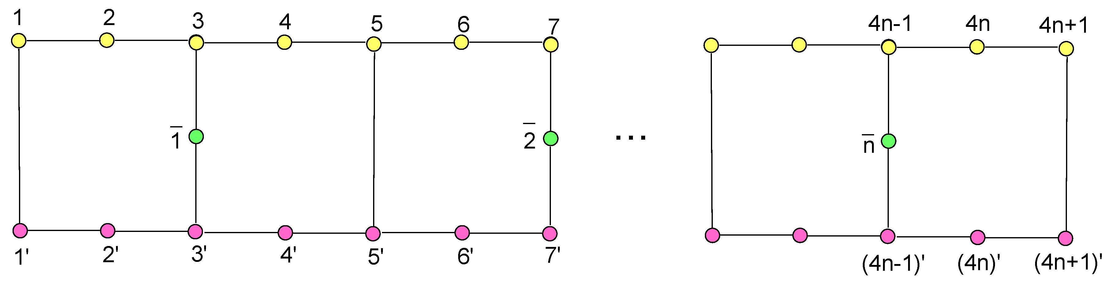
Let $H_n$ be the heptagonal networks as illustrated in Figure 1, of which two heptagons have two common edges. That is, two heptagons can be seen as adding two $P_2$ and attaching them. Notice that there are some applications of the heptagons derived from different aspects, which are listed as follows. The 20p and 50p coins of the United Kingdom have two heptagons. Although there are less heptagonal floor plans, a remarkable example is the Mausoleum of Prince Ernst. Meanwhile, cacti are the most common plants with heptagons in natural structures.

For the exited results of linear networks [20,21,22,23], there were only two types of vertices considered in these paper. The structure of linear heptagonal networks is much more complex, of which have three types of vertices, shown in Figure 1. It was challenging and meaningful for us to study the structural properties of linear heptagonal networks. On the other hand, the degree-Kirchhoff index and the number of spanning trees are the important parameters to predict the structure properties of graphs. Therefore, computing the degree-Kirchhoff index and the number of spanning trees of linear heptagonal networks are interesting works. In the rest of the context, we recall some necessary notations and methods used in the proofs of the main results in Section 2. We aimed to first determine the normalized Laplacian spectrum of $H_n$ by the decomposition theorem for the normalized Laplacian matrix of $H_n$. We then derived the explicit formulas for the degree-Kirchhoff index and the number of spanning trees of $H_n$ through using the relationships between the roots and coefficients in Section 3. The discussion of the previous results is given in Section 4. A conclusion is summarized in Section 5.

2. Materials and Methods

In this section, we first recall some basic notations and introduce a classical method, which laid the foundations for this paper. All equations that we introduce below can be found in Reference [1,19].

Fix a square matrix M with order n, denote the submatrix of M the $M[i_1,\dots ,i_k]$, and yield by the deletion of the $i_1$-th, …, $i_k$-th rows and corresponding columns. Assume that $P_M\left(x\right)=det(xI-M)$ is the characteristic polynomial of the $n\times n$ matrix M.

Let $H_n$ be the graph, as illustrated in Figure 1, with $V_0=\{\overline{1},\overline{2},\dots ,\overline{n}\}$,$V_1=\{1,2,\dots ,4n+1\}$ and $V_2=\{1^{\prime },2^{\prime },\dots ,{(4n+1)}^{\prime }\}$. It is straightforward to verify that $\pi =\left(\overline{1}\right)\left(\overline{2}\right)\cdots \left(\overline{n}\right)(1,1^{\prime })(2,2^{\prime })\cdots (4n+1,{(4n+1)}^{\prime })$ is an automorphism. Then the normalized laplacian matrix of $H_n$ can be given as the following block matrices.

$$\mathcal{L}\left(H_n\right)=\left(\begin{array}{ccc}{\mathcal{L}}_{V_0{V}_0}& {\mathcal{L}}_{V_0{V}_1}& {\mathcal{L}}_{V_0{V}_2}\\ {\mathcal{L}}_{V_1{V}_0}& {\mathcal{L}}_{V_1{V}_1}& {\mathcal{L}}_{V_1{V}_2}\\ {\mathcal{L}}_{V_2{V}_0}& {\mathcal{L}}_{V_2{V}_1}& {\mathcal{L}}_{V_2{V}_2}\end{array}\right).$$

(4)

Notice that, ${\mathcal{L}}_{V_0{V}_1}={\mathcal{L}}_{V_0{V}_2},{\mathcal{L}}_{V_1{V}_0}={\mathcal{L}}_{V_2{V}_0},{\mathcal{L}}_{V_1{V}_1}={\mathcal{L}}_{V_2{V}_2}$ and ${\mathcal{L}}_{V_1{V}_2}={\mathcal{L}}_{V_2{V}_1}$.

Given:

$$T=\left(\begin{array}{ccc}{I}_n& 0& 0\\ 0& \frac{1}{\sqrt{2}}{I}_n& \frac{1}{\sqrt{2}}{I}_n\\ 0& \frac{1}{\sqrt{2}}{I}_n& -\frac{1}{\sqrt{2}}{I}_n\end{array}\right),$$

then

$$T\mathcal{L}\left(H_n\right)T^{\prime }=\left(\begin{array}{cc}{\mathcal{L}}_A& 0\\ 0& {\mathcal{L}}_S\end{array}\right),$$

(5)

where $T^{\prime }$ is the transposition of T.

$${\mathcal{L}}_A=\left(\begin{array}{cc}{I}_n& \sqrt{2}{\mathcal{L}}_{V_0{V}_1}\\ \sqrt{2}{\mathcal{L}}_{V_1{V}_0}& {\mathcal{L}}_{V_1{V}_1}+{\mathcal{L}}_{V_1{V}_2}\end{array}\right),{\mathcal{L}}_s={\mathcal{L}}_{V_1{V}_1}-{\mathcal{L}}_{V_1{V}_2}.$$

(6)

At this place, the matrices introduced above are given in the following. In view of Equation (1) and Figure 1, one has ${\mathcal{L}}_{V_0{V}_0}=I_n$.

$$\begin{array}{ccc}{\mathcal{L}}_{V_0{V}_1}\hfill & =& {\left(l_{ij}\right)}_{n\times (4n+1)}\hfill \\ & =& {\left(\begin{array}{ccccccccccc}0& 0& -\frac{1}{\sqrt{6}}& 0& 0& 0& 0& \cdots & 0& 0& 0\\ 0& 0& 0& 0& 0& 0& -\frac{1}{\sqrt{6}}& \cdots & 0& 0& 0\\ 0& 0& 0& 0& 0& 0& 0& \cdots & 0& 0& 0\\ ⋮& ⋮& ⋮& ⋮& ⋮& ⋮& ⋮& \ddots & ⋮& ⋮& ⋮\\ 0& 0& 0& 0& 0& 0& 0& \cdots & 0& 0& 0\\ 0& 0& 0& 0& 0& 0& 0& \cdots & -\frac{1}{\sqrt{6}}& 0& 0\end{array}\right)}_{n\times (4n+1)},\hfill \end{array}$$

where $l_{ij}=-\frac{1}{\sqrt{6}}$ and $l_{ij}=0$, if $j=4i-1$ and otherwise, respectively.

$$\begin{array}{c}\hfill {\mathcal{L}}_{V_1{V}_1}={\left(\begin{array}{cccccccc}1& -\frac{1}{2}& 0& 0& \cdots & 0& 0& 0\\ -\frac{1}{2}& 1& \frac{-1}{\sqrt{6}}& 0& \cdots & 0& 0& 0\\ 0& \frac{-1}{\sqrt{6}}& 1& \frac{-1}{\sqrt{6}}& \cdots & 0& 0& 0\\ 0& 0& \frac{-1}{\sqrt{6}}& 1& \cdots & 0& 0& 0\\ ⋮& ⋮& ⋮& ⋮& \ddots & ⋮& ⋮& ⋮\\ 0& 0& 0& 0& \cdots & 1& \frac{-1}{\sqrt{6}}& 0\\ 0& 0& 0& 0& \cdots & \frac{-1}{\sqrt{6}}& 1& -\frac{1}{2}\\ 0& 0& 0& 0& \cdots & 0& -\frac{1}{2}& 1\end{array}\right)}_{(4n+1)\times (4n+1)}.\end{array}$$

On the other hand, one gets:

$${\mathcal{L}}_{V_1{V}_2}={\left(l_{ij}\right)}_{(4n+1)\times (4n+1)}=diag(-\frac{1}{2},0,0,0,-\frac{1}{3},\dots ,-\frac{1}{3},0,0,0,-\frac{1}{2}),$$

where $l_{11}=l_{4n+1,4n+1}=-\frac{1}{2}$, $l_{4k+1,4k+1}=-\frac{1}{3}$ for $k\in \{1,2,\dots ,n-1\}$ and 0 otherwise.

According to Equation (5), one has:

$$\begin{array}{ccc}{\mathcal{L}}_{V_1{V}_1}+{\mathcal{L}}_{V_1{V}_2}\hfill & =& {\left(l_{ij}\right)}_{(4n+1)\times (4n+1)}\hfill \\ & =& {\left(\begin{array}{ccccccccc}\frac{1}{2}& -\frac{1}{2}& 0& 0& 0& \cdots & 0& 0& 0\\ -\frac{1}{2}& 1& \frac{-1}{\sqrt{6}}& 0& 0& \cdots & 0& 0& 0\\ 0& \frac{-1}{\sqrt{6}}& 1& \frac{-1}{\sqrt{6}}& 0& \cdots & 0& 0& 0\\ 0& 0& \frac{-1}{\sqrt{6}}& 1& \frac{-1}{\sqrt{6}}& \cdots & 0& 0& 0\\ 0& 0& 0& \frac{-1}{\sqrt{6}}& \frac{2}{3}& \cdots & 0& 0& 0\\ ⋮& ⋮& ⋮& ⋮& ⋮& \ddots & ⋮& ⋮& ⋮\\ 0& 0& 0& 0& 0& \cdots & 1& \frac{-1}{\sqrt{6}}& 0\\ 0& 0& 0& 0& 0& \cdots & \frac{-1}{\sqrt{6}}& 1& -\frac{1}{2}\\ 0& 0& 0& 0& 0& \cdots & 0& -\frac{1}{2}& \frac{1}{2}\end{array}\right)}_{(4n+1)\times (4n+1)},\hfill \end{array}$$

where $l_{11}=l_{4n+1,4n+1}=\frac{1}{2}$, $l_{ii}=1$ for $i\in \{2,3,\dots ,4n\}$ and $i\ne 4k+1$, $l_{4k+1,4k+1}=\frac{2}{3}$ for $k\in \{1,2,\dots ,n-1\}$. Also, $l_{12}=l_{21}=l_{4n,4n+1}=l_{4n+1,4n}=-\frac{1}{2}$, $l_{i,i+1}=l_{i+1,i}=-\frac{1}{\sqrt{6}}$ for $i\in \{2,3,\dots ,4n-1\}$ and $l_{ij}=0$ for $|i-j|>1$.

And:

$$\begin{array}{ccc}{\mathcal{L}}_S\hfill & =& {\left(l_{ij}\right)}_{(4n+1)\times (4n+1)}\hfill \\ & =& {\left(\begin{array}{ccccccccc}\frac{3}{2}& -\frac{1}{2}& 0& 0& 0& \cdots & 0& 0& 0\\ -\frac{1}{2}& 1& \frac{-1}{\sqrt{6}}& 0& 0& \cdots & 0& 0& 0\\ 0& \frac{-1}{\sqrt{6}}& 1& \frac{-1}{\sqrt{6}}& 0& \cdots & 0& 0& 0\\ 0& 0& \frac{-1}{\sqrt{6}}& 1& \frac{-1}{\sqrt{6}}& \cdots & 0& 0& 0\\ 0& 0& 0& \frac{-1}{\sqrt{6}}& \frac{4}{3}& \cdots & 0& 0& 0\\ ⋮& ⋮& ⋮& ⋮& ⋮& \ddots & ⋮& ⋮& ⋮\\ 0& 0& 0& 0& 0& \cdots & 1& \frac{-1}{\sqrt{6}}& 0\\ 0& 0& 0& 0& 0& \cdots & \frac{-1}{\sqrt{6}}& 1& -\frac{1}{2}\\ 0& 0& 0& 0& 0& \cdots & 0& -\frac{1}{2}& \frac{3}{2}\end{array}\right)}_{(4n+1)\times (4n+1)},\hfill \end{array}$$

where $l_{11}=l_{4n+1,4n+1}=\frac{3}{2}$, $l_{ii}=1$ for $i\in \{2,3,\dots ,4n\}$ and $i\ne 4k+1$, $l_{4k+1,4k+1}=\frac{4}{3}$ for $k\in \{1,2,\dots ,n-1\}$. Also, $l_{12}=l_{21}=l_{4n,4n+1}=l_{4n+1,4n}=-\frac{1}{2}$, $l_{i,i+1}=l_{i+1,i}=-\frac{1}{\sqrt{6}}$ for $i\in \{2,3,\dots ,4n-1\}$ and $l_{ij}=0$ for $|i-j|>1$.

In what follows, the lemmas that we present will be used throughout the main results.

Lemma 1.

Assume that ${\mathcal{L}}_A,{\mathcal{L}}_s$ are defined as mentioned above [1]. Then:

$$P_{\mathcal{L}\left(L_n\right)}\left(x\right)=P_{{\mathcal{L}}_A}\left(x\right)P_{{\mathcal{L}}_s}\left(x\right).$$

According to the relation between the number of spanning trees and its normalized laplacian eigenvalues, one arrives the following lemma.

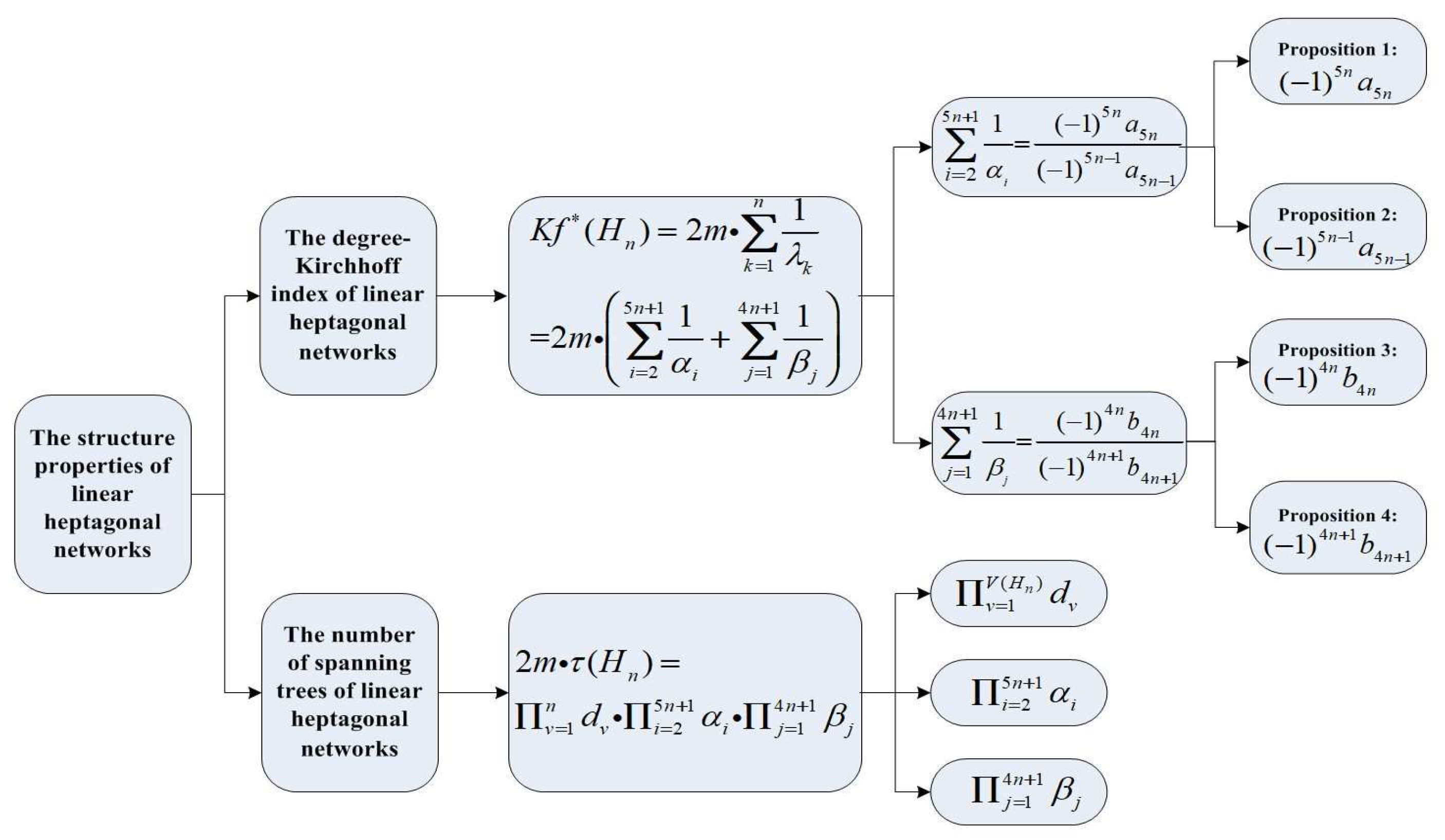
Lemma 2.

Assume that G is a connected graph with order n and size m [7], then

$$\prod _{i=1}^n{d}_G\left(v_i\right)\prod _{i=2}^n{\lambda }_i=2m\tau \left(G\right),$$

where $\tau \left(G\right)$ is the number of spanning trees of G.

Lemma 3.

Let $M_1,M_2,M_3$ and $M_4$ be the $p\times p$, $p\times q$, $q\times p$ and $q\times q$ matrices, respectively [24]. Then:

$$\begin{array}{c}\left(a\right).det\left(\begin{array}{cc}{M}_1& M_2\\ M_3& M_4\end{array}\right)=det\left(M_4\right)·det\left(M_1-M_2{M}_4^{-1}{M}_3\right),\hfill \\ \left(b\right).det\left(\begin{array}{cc}{M}_1& M_2\\ M_3& M_4\end{array}\right)=det\left(M_1\right)·det\left(M_4-M_3{M}_1^{-1}{M}_2\right),\hfill \\ \hfill \end{array}$$

where $M_1$ and $M_4$ are invertible, and $M_1-M_2{M}_4^{-1}{M}_3$ and $M_4-M_3{M}_1^{-1}{M}_2$ are called the Schur complements of $M_4$ and $M_1$, respectively.

In what follows, a flowchart (Figure 2) is given on the basis of the steps we have processed, and it will facilitate the understanding of the proposed approach. The explanations of these notations that appear in the flowchart are presented in Section 3.

3. Main Results

In this section, we first figure out the explicit formula for the degree-Kirchhoff index of $H_n$. The steps of computing the degree-Kirchhoff index follow the flowchart in Figure 2. Combining the eigenvalues of ${\mathcal{L}}_A$ and ${\mathcal{L}}_s$, it is easy to get the normalized Laplacian spectrum of $H_n$ by Lemma 1. On the other hand, one can find that the number or spanning trees of $H_n$ consists of the products of the degree of all vertices, the eigenvalues of ${\mathcal{L}}_A$ and ${\mathcal{L}}_s$, respectively. Suppose $0={\alpha }_1<{\alpha }_2\le \cdots \le {\alpha }_{5n+1}$ and $0<{\beta }_1\le {\beta }_2\le \cdots \le {\beta }_{4n+1}$ are the roots of $P_{{\mathcal{L}}_A}\left(x\right)=0$ and $P_{L_s}\left(x\right)=0$, respectively. By Equation (3), one has:

Lemma 4.

Suppose that $H_n$ are the linear heptagonal networks. Then:

$$\begin{array}{ccc}\hfill K{f}^{*}\left(H_n\right)& =& 2·(11n+1)·(\sum _{i=2}^{5n+1}\frac{1}{{\alpha }_i}+\sum _{j=1}^{4n+1}\frac{1}{{\beta }_j}).\hfill \end{array}$$

(7)

Evidently, one just needs to calculate the eigenvalues of the ${\mathcal{L}}_A$ and ${\mathcal{L}}_S$. Hence, the formulas of ${\sum }_{i=2}^{5n+1}\frac{1}{{\alpha }_i}$ and ${\sum }_{j=1}^{4n+1}\frac{1}{{\beta }_j}$ are given in the following lemmas.

Lemma 5.

Suppose that $0={\alpha }_1<{\alpha }_2\le \cdots \le {\alpha }_{5n+1}$ are the eigenvalues of ${\mathcal{L}}_A$. One has:

$$\sum _{i=2}^{5n+1}\frac{1}{{\alpha }_i}=\frac{401n^3-170n^2+54n}{11n+1}.$$

Proof. 

It is straightforward to verify that:

$$P_{{\mathcal{L}}_A}\left(x\right)=x^{5n+1}+a_1{x}^{5n}+\cdots +a_{5n-1}{x}^2+a_{5n}x=x(x^{5n}+a_1{x}^{5n-1}+\cdots +a_{5n-1}x+a_{5n}),$$

with $a_{5n}\ne 0.$ Then, one knows that $\frac{1}{{\alpha }_2},\frac{1}{{\alpha }_3},\dots ,\frac{1}{{\alpha }_{5n+1}}$ are the roots of the following equation:

$$a_{5n}·x^{5n}+a_{5n-1}·x^{5n-1}+\cdots +a_1·x+1=0.$$

According to the relationships between the roots and the coefficients and Vieta theorem, one arrives at:

$$\begin{array}{c}\hfill \sum _{i=2}^{5n+1}\frac{1}{{\alpha }_i}=\frac{{(-1)}^{5n-1}·a_{5n-1}}{{(-1)}^{5n}·a_{5n}}.\end{array}$$

□

Proposition 1.

${(-1)}^{5n}·a_{5n}=\frac{11n+1}{8}{\left(\frac{1}{6}\right)}^{2n-1}.$

Proof. 

Since the number ${(-1)}^{5n}{a}_{5n}$ is the sum of all those principal minors of ${\mathcal{L}}_A$ which have $5n$ rows and columns, we get:

$$\begin{array}{c}\hfill {(-1)}^{5n}·a_{5n}=\sum _{i=1}^{5n+1}det{\mathcal{L}}_A\left[i\right].\end{array}$$

(8)

In view of Equation (6), one may find that i can be selected in the identity matrix $I_n$ or ${\mathcal{L}}_{V_1{V}_1}+{\mathcal{L}}_{V_1{V}_2}.$ Thus, all these cases are listed as below.

Case 1. One first considers the case $1\le i\le n.$ That is to say, ${\mathcal{L}}_A\left[i\right]$ is obtained by deleting the i row of the identity matrix $I_n$ and $\sqrt{2}{\mathcal{L}}_{V_0{V}_1}$, and also the corresponding column of the $I_n$ and $\sqrt{2}{\mathcal{L}}_{V_1{V}_0}.$ Denoted by $I_{n-1},R_{(n-1)\times (4n+1)},R_{(n-1)\times (4n+1)}^{\prime }$ and $U_{(4n+1)\times (4n+1)}$ are the resulting blocks, respectively. According to the Lemma 3, and applying elementary operations (see also in Reference [25], P8), one knows:

$$\begin{array}{c}\hfill det{\mathcal{L}}_A\left[i\right]=\left|\begin{array}{cc}{I}_{n-1}& R_{(n-1)\times (4n+1)}\\ R_{(n-1)\times (4n+1)}^{\prime }& U_{(4n+1)\times (4n+1)}\end{array}\right|=\left|\begin{array}{cc}{I}_{n-1}& 0\\ 0& M_1\end{array}\right|,\end{array}$$

where $M_1=U_{(4n+1)\times (4n+1)}-R_{(n-1)\times (4n+1)}^{\prime }{R}_{(n-1)\times (4n+1)}=\left(m_{pq}\right),$ of which $m_{11}=m_{4n+1,4n+1}=\frac{1}{2},m_{pp}=1$ for $p\in \{2,4,6,\dots ,4n\},$ $m_{pp}=\frac{2}{3}$ for $p\in \{3,5,7,4n-1\}$ but $p\ne 4i-1,$ $m_{4i-1,4i-1}=1.$ Also, $m_{12}=m_{21}=m_{4n,4n+1}=m_{4n+1,4n}=-\frac{1}{2}$, $m_{p,p+1}=m_{p+1,p}=-\frac{1}{\sqrt{6}}$ for $p\in \{2,3,\dots ,4n-1\}$ and $m_{pq}=0$ for $|p-q|>1$. With a explicit calculation, one gets:

$$\begin{array}{c}\hfill det{\mathcal{L}}_A\left[i\right]=det{M}_1=\frac{1}{8}\times {\left(\frac{1}{6}\right)}^{2n-1}.\end{array}$$

(9)

Case 2. One now takes into account the case $n+1\le i\le 5n+1.$ Namely, ${\mathcal{L}}_A\left[i\right]$ is obtained by deleting the i row of the ${\mathcal{L}}_{V_1{V}_1}+{\mathcal{L}}_{V_1{V}_2}$ and $\sqrt{2}{\mathcal{L}}_{V_1{V}_0}$, also the corresponding column of the ${\mathcal{L}}_{V_1{V}_1}+{\mathcal{L}}_{V_1{V}_2}$ and $\sqrt{2}{\mathcal{L}}_{V_0{V}_1}.$ Denote by $I_n,R_{n\times 4n},R_{n\times 4n}^{\prime }$ and $U_{4n\times 4n}$ the resulting blocks, respectively. According to Lemma 3 and applying elementary operations, we arrive at:

$$\begin{array}{c}\hfill det{\mathcal{L}}_A\left[i\right]=\left|\begin{array}{cc}{I}_n& R_{n\times 4n}\\ R_{n\times 4n}^{\prime }& U_{4n\times 4n}\end{array}\right|=\left|\begin{array}{cc}{I}_n& 0\\ 0& M_2\end{array}\right|,\end{array}$$

where $M_2=U_{4n\times 4n}-R_{n\times 4n}^{\prime }{R}_{n\times 4n}.$ Set $M_{2^{\prime }}=\left(m_{pq}\right)$ with order $4n+1$, of which $m_{11}=m_{4n+1,4n+1}=\frac{1}{2},m_{pp}=1$ for $p\in \{2,4,6,\dots ,4n\},$ $m_{pp}=\frac{2}{3}$ for $p\in \{3,5,7,4n-1\}$. Also, $m_{12}=m_{21}=m_{4n,4n+1}=m_{4n+1,4n}=-\frac{1}{2}$, $m_{p,p+1}=m_{p+1,p}=-\frac{1}{\sqrt{6}}$ for $p\in \{2,3,\dots ,4n-1\}$ and $m_{pq}=0$ for $|p-q|>1$. Evidently, $M_2=M_{2^{\prime }}[i-n]$. With an explicit calculation, one gets:

$$\begin{array}{c}\hfill det{\mathcal{L}}_A\left[i\right]=det{M}_{2^{\prime }}[i-n]=\left\{\begin{array}{cc}\frac{1}{4}\times {\left(\frac{1}{6}\right)}^{2n-1},\hfill & ifi=n+1ori=5n+1;\hfill \\ \frac{1}{4}\times {\left(\frac{1}{6}\right)}^{2n-1},\hfill & ifn+2\le i\le 5n,iiseven;\hfill \\ \frac{1}{16}\times {\left(\frac{1}{6}\right)}^{2n-2},\hfill & ifn+2\le i\le 5n,iisodd.\hfill \end{array}\right.\end{array}$$

(10)

Combining Equations (8)–(10), we have:

$$\begin{array}{ccc}{(-1)}^{5n}·a_{5n}\hfill & =& \sum _{i=1}^{5n+1}det{\mathcal{L}}_A\left[i\right]=\sum _{i=1}^{n}det{\mathcal{L}}_A\left[i\right]+\sum _{i=n+1}^{5n+1}det{\mathcal{L}}_A\left[i\right]\hfill \\ & =& n·\frac{1}{8}\times {\left(\frac{1}{6}\right)}^{2n-1}+2n·\frac{1}{4}\times {\left(\frac{1}{6}\right)}^{2n-1}+(2n-1)·\frac{1}{16}\times {\left(\frac{1}{6}\right)}^{2n-2}+2\times \frac{1}{4}\times {\left(\frac{1}{6}\right)}^{2n-1}\hfill \\ & =& \frac{11n+1}{8}·{\left(\frac{1}{6}\right)}^{2n-1}.\hfill \end{array}$$

This completes the proof of the Proposition 1. □

In what follows, we will focus on the calculation of the ${(-1)}^{5n-1}{a}_{5n-1}$.

Proposition 2.

${(-1)}^{5n-1}{a}_{5n-1}=\frac{1}{48}(401n^3-170n^2+54n){\left(\frac{1}{6}\right)}^{2n-2}.$

Proof. 

Since the number ${(-1)}^{5n-1}{a}_{5n-1}$ is the sum of all those principal minors of ${\mathcal{L}}_A$ which have $5n-1$ rows and columns, it is straightforward to obtain that:

$$\begin{array}{c}\hfill {(-1)}^{5n-1}·a_{5n-1}=\sum _{i=1}^{5n+1}det{\mathcal{L}}_A[i,j].\end{array}$$

(11)

Similar to consideration of Proposition 1, all these cases are listed as follows.

Case 1. One first considers the case $1\le i<j\le n.$ That is to say, ${\mathcal{L}}_A[i,j]$ is obtained by deleting the i and j rows of the identity matrix $I_n$ and $\sqrt{2}{\mathcal{L}}_{V_0{V}_1}$, also the corresponding columns of the $I_n$ and $\sqrt{2}{\mathcal{L}}_{V_1{V}_0}.$ Denote by $I_{n-2},R_{(n-2)\times (4n+1)},R_{(n-2)\times (4n+1)}^{\prime }$ and $U_{(4n+1)\times (4n+1)}$ the resulting blocks, respectively. According to Lemma 3 and applying elementary operations, one has:

$$\begin{array}{c}\hfill det{\mathcal{L}}_A[i,j]=\left|\begin{array}{cc}{I}_{n-2}& R_{(n-2)\times (4n+1)}\\ R_{(n-2)\times (4n+1)}^{\prime }& U_{(4n+1)\times (4n+1)}\end{array}\right|=\left|\begin{array}{cc}{I}_{n-2}& 0\\ 0& M_3\end{array}\right|,\end{array}$$

where $M_3=U_{(4n+1)\times (4n+1)}-R_{(n-2)\times (4n+1)}^{\prime }{R}_{(n-2)\times (4n+1)}=\left(m_{pq}\right),$ of which $m_{11}=m_{4n+1,4n+1}=\frac{1}{2},m_{pp}=1$ for $p\in \{2,4,6,\dots ,4n\},$ $m_{pp}=\frac{2}{3}$ for $p\in \{3,5,7,4n-1\}$ but $p\ne 4i-1$ and $p\ne 4j-1$, $m_{4i-1,4i-1}=m_{4j-1,4j-1}=1.$ Also, $m_{12}=m_{21}=m_{4n,4n+1}=m_{4n+1,4n}=-\frac{1}{2}$, $m_{p,p+1}=m_{p+1,p}=-\frac{1}{\sqrt{6}}$ for $p\in \{2,3,\dots ,4n-1\}$ and $m_{pq}=0$ for $|p-q|>1$. With an explicit calculation, one gets:

$$\begin{array}{c}\hfill det{\mathcal{L}}_A[i,j]=det{M}_3=\frac{1}{8}·(j-i+2)·{\left(\frac{1}{6}\right)}^{2n-1}.\end{array}$$

(12)

Case 2. One now takes into account the case $n+1\le i<j\le 5n+1.$ Namely, ${\mathcal{L}}_A[i,j]$ is obtained by deleting the $(i-n)$-th and $(j-n)$-th rows of the ${\mathcal{L}}_{V_1{V}_1}+{\mathcal{L}}_{V_1{V}_2}$ and $\sqrt{2}{\mathcal{L}}_{V_1{V}_0}$, also the corresponding columns of the ${\mathcal{L}}_{V_1{V}_1}+{\mathcal{L}}_{V_1{V}_2}$ and $\sqrt{2}{\mathcal{L}}_{V_0{V}_1}.$ Denote by $I_n,R_{n\times (4n-1)},R_{n\times (4n-1)}^{\prime }$ and $U_{(4n-1)\times (4n-1)}$ the resulting blocks, respectively. According to Lemma 3 and applying elementary operations, one arrives at:

$$\begin{array}{c}\hfill det{\mathcal{L}}_A[i,j]=\left|\begin{array}{cc}{I}_n& R_{n\times (4n-1)}\\ R_{n\times (4n-1)}^{\prime }& U_{(4n-1)\times (4n-1)}\end{array}\right|=\left|\begin{array}{cc}{I}_n& 0\\ 0& M_4\end{array}\right|,\end{array}$$

where $M_4=U_{(4n-1)\times (4n-1)}-R_{n\times (4n-1)}^{\prime }{R}_{n\times (4n-1)}=M_{2^{\prime }}[i-n,j-n]$. With an explicit calculation, one gets:

$$\begin{array}{c}\hfill det{\mathcal{L}}_A[i,j]=\left\{\begin{array}{cc}\frac{1}{8}(j-i){\left(\frac{1}{6}\right)}^{2n-2},\hfill & ifn+2\le i=n+l<j=n+k\le 5n,liseven,kisodd;\hfill \\ \frac{1}{12}(j-i){\left(\frac{1}{6}\right)}^{2n-2},\hfill & ifn+2\le i=n+l<j=n+k\le 5n,liseven,kiseven;\hfill \\ \frac{1}{8}(j-i){\left(\frac{1}{6}\right)}^{2n-2},\hfill & ifn+2\le i=n+l<j=n+k\le 5n,lisodd,kiseven;\hfill \\ \frac{3}{16}(j-i){\left(\frac{1}{6}\right)}^{2n-2},\hfill & ifn+2\le i=n+l<j=n+k\le 5n,lisodd,kisodd;\hfill \\ \frac{1}{8}(j-i){\left(\frac{1}{6}\right)}^{2n-2},\hfill & ifi=n+1,j=n+k,kisodd;\hfill \\ \frac{1}{6}(j-i){\left(\frac{1}{6}\right)}^{2n-2},\hfill & ifi=n+1,j=n+k,kiseven;\hfill \\ \frac{1}{8}(j-i){\left(\frac{1}{6}\right)}^{2n-2},\hfill & ifi=n+k,j=5n+1,kisodd;\hfill \\ \frac{1}{12}(j-i){\left(\frac{1}{6}\right)}^{2n-2},\hfill & ifi=n+k,j=5n+1,kiseven;\hfill \\ 2n{\left(\frac{1}{6}\right)}^{2n-1},\hfill & ifi=n+1,j=5n+1.\hfill \end{array}\right.\end{array}$$

(13)

Case 3. One devotes to consideration of the case $1\le i\le n$, $n+1\le j\le 5n+1$. That is, ${\mathcal{L}}_A[i,j]$ is obtained by deleting the i rows of the identity matrix $I_n$ and $\sqrt{2}{\mathcal{L}}_{V_0{V}_1}$, $(j-n)$-th rows of the $\sqrt{2}{\mathcal{L}}_{V_1{V}_0}$ and ${\mathcal{L}}_{V_1{V}_1}+{\mathcal{L}}_{V_1{V}_2}$, respectively. In addition, the corresponding columns of the $I_n$, $\sqrt{2}{\mathcal{L}}_{V_1{V}_0}$, ${\mathcal{L}}_{V_1{V}_1}+{\mathcal{L}}_{V_1{V}_2}$ and $\sqrt{2}{\mathcal{L}}_{V_0{V}_1}.$ Denote by $I_{n-1},R_{(n-1)\times 4n},R_{(n-1)\times 4n}^{\prime }$ and $U_{4n\times 4n}$ the resulting blocks, respectively. According to Lemma 3 and applying elementary operations, one has:

$$\begin{array}{c}\hfill det{\mathcal{L}}_A[i,j]=\left|\begin{array}{cc}{I}_{n-1}& R_{(n-1)\times 4n}\\ R_{(n-1)\times 4n}^{\prime }& U_{4n\times 4n}\end{array}\right|=\left|\begin{array}{cc}{I}_n& 0\\ 0& M_5\end{array}\right|,\end{array}$$

where $M_5=U_{4n\times 4n}-R_{(n-1)\times 4n}^{\prime }{R}_{(n-1)\times 4n}=M_1[j-n]$. By an explicit calculation, we get:

$$\begin{array}{c}\hfill det{\mathcal{L}}_A[i,j]=\left\{\begin{array}{cc}(\frac{1}{2}+i){\left(\frac{1}{6}\right)}^{2n-1},\hfill & ifj=n+1;\hfill \\ \frac{1}{24}(j-n-2i){\left(\frac{1}{6}\right)}^{2n-2},\hfill & ifn+2\le j=n+k\le 5n,j-n-2i>0,kiseven;\hfill \\ \frac{1}{12}{\left(\frac{1}{6}\right)}^{2n-2},\hfill & ifn+2\le j=n+k\le 5n,j-n-2i=0,kiseven;\hfill \\ \frac{1}{12}\left(\right|\frac{j-n-2i}{2}|+1){\left(\frac{1}{6}\right)}^{2n-2},\hfill & ifn+2\le j=n+k\le 5n,j-n-2i<0,kiseven;\hfill \\ \frac{1}{16}(j-n-2i){\left(\frac{1}{6}\right)}^{2n-2},\hfill & ifn+2\le j=n+k\le 5n,j-n-2i\ge 0,kisodd;\hfill \\ \frac{1}{16}\left(\right|j-n-2i|+2){\left(\frac{1}{6}\right)}^{2n-2},\hfill & ifn+2\le j=n+k\le 5n,j-n-2i<0,kisodd;\hfill \\ \frac{1}{4}(4n-2i+1){\left(\frac{1}{6}\right)}^{2n-1},\hfill & ifj=5n+1.\hfill \end{array}\right.\end{array}$$

(14)

Together with Equations (11)–(14), one gets:

$$\begin{array}{ccc}{(-1)}^{5n-1}{a}_{5n-1}\hfill & =& \sum _{1\le i\le j}^{5n+1}det{\mathcal{L}}_A[i,j]\hfill \\ & =& \sum _{1\le i\le j}^{n}det{\mathcal{L}}_A[i,j]+\sum _{n+1\le i\le j}^{5n+1}det{\mathcal{L}}_A[i,j]+\sum _{1\le i\le n,n+1\le j\le 5n+1}^{5n+1}det{\mathcal{L}}_A[i,j]\hfill \\ & =& \frac{n^3+12n^2+11n}{48}{\left(\frac{1}{6}\right)}^{2n-1}+\frac{290n^3-144n^2+25n}{36}{\left(\frac{1}{6}\right)}^{2n-2}\hfill \\ & & +\frac{40n^3+30n^2+29n}{144}{\left(\frac{1}{6}\right)}^{2n-2}\hfill \\ & =& \frac{1}{48}(401n^3-170n^2+54n){\left(\frac{1}{6}\right)}^{2n-2}.\hfill \end{array}$$

The proof of the Proposition 2 completed. □

By Propositions 1 and 2, we have the desired result of Lemma 5.

Lemma 6.

Suppose that ${\beta }_1,{\beta }_2,\dots ,{\beta }_{4n+1}$ are the eigenvalues of ${\mathcal{L}}_S$. One has:

$$\sum _{j=1}^{4n+1}\frac{1}{{\beta }_j}=\frac{\delta \left(n\right)+\zeta \left(n\right)}{441\left[(-24+2183\sqrt{2}){(11-6\sqrt{2})}^n-(24+2183\sqrt{2}){(11+6\sqrt{2})}^n\right]},$$

where $\delta \left(n\right)=4\left(461133-44560\sqrt{2}-6n(249938+99525\sqrt{2})\right){(11+6\sqrt{2})}^n,$$\zeta \left(n\right)=4\left(461133+44560\sqrt{2}+6n(-249938+99525\sqrt{2})\right){(11-6\sqrt{2})}^n$.

Proof. 

It is straightforward to verify that:

$$P_{{\mathcal{L}}_S}\left(x\right)=x^{4n+1}+b_1{x}^{4n}+\cdots +b_{4n-1}{x}^2+b_{4n}x+b_{4n+1},$$

with $b_{4n+1}\ne 0.$ Then, one knows that $\frac{1}{{\beta }_1},\frac{1}{{\beta }_2},\dots ,\frac{1}{{\beta }_{4n+1}}$ are the roots of the following equation:

$$b_{4n+1}·x^{4n+1}+b_{4n}·x^{4n}+\cdots +b_1·x+1=0.$$

In the line with the relationships between the roots and the coefficients of $P_{{\mathcal{L}}_s}\left(x\right)$, one arrives at:

$$\begin{array}{c}\hfill \sum _{j=1}^{4n+1}\frac{1}{{\beta }_j}=\frac{{(-1)}^{4n}{b}_{4n}}{{(-1)}^{4n+1}{b}_{4n+1}}=\frac{{(-1)}^{4n}{b}_{4n}}{det{\mathcal{L}}_s}.\end{array}$$

On the one hand, we first consider l-th order principal submatrix, $D_l$, and yield by the first l rows and columns of ${\mathcal{L}}_s,l=1,2,\dots ,4n$. Set $d_l=det{D}_l$. Then $d_1=\frac{3}{2},d_2=\frac{5}{4},d_3=1,d_4=\frac{19}{24},d_5=\frac{8}{9},d_6=\frac{109}{144},d_7=\frac{263}{432},d_8=\frac{139}{288}$ and:

$$\begin{array}{c}\hfill \left\{\begin{array}{c}{d}_{4i}=d_{4i-1}-\frac{1}{6}{d}_{4i-2},\hfill \\ d_{4i+1}=\frac{4}{3}{d}_{4i}-\frac{1}{6}{d}_{4i-1},\hfill \\ d_{4i+2}=d_{4i+1}-\frac{1}{6}{d}_{4i},\hfill \\ d_{4i+3}=d_{4i+2}-\frac{1}{6}{d}_{4i+1}.\hfill \end{array}\right.\end{array}$$

(15)

With a explicit calculation, we get:

$$\begin{array}{c}\hfill \left\{\begin{array}{c}{d}_{4i}=\frac{460+3\sqrt{2}}{196\sqrt{2}}{\left(\frac{11+6\sqrt{2}}{36}\right)}^i+\frac{-460+3\sqrt{2}}{196\sqrt{2}}{\left(\frac{11-6\sqrt{2}}{36}\right)}^i,\hfill \\ d_{4i+1}=\frac{31+18\sqrt{2}}{24\sqrt{2}}{\left(\frac{11+6\sqrt{2}}{36}\right)}^i+\frac{-31+18\sqrt{2}}{24\sqrt{2}}{\left(\frac{11-6\sqrt{2}}{36}\right)}^i,\hfill \\ d_{4i+2}=\frac{27+15\sqrt{2}}{24\sqrt{2}}{\left(\frac{11+6\sqrt{2}}{36}\right)}^i+\frac{-27+15\sqrt{2}}{24\sqrt{2}}{\left(\frac{11-6\sqrt{2}}{36}\right)}^i,\hfill \\ d_{4i+3}=\frac{131+72\sqrt{2}}{144\sqrt{2}}{\left(\frac{11+6\sqrt{2}}{36}\right)}^i+\frac{-131+72\sqrt{2}}{144\sqrt{2}}{\left(\frac{11-6\sqrt{2}}{36}\right)}^i.\hfill \end{array}\right.\end{array}$$

(16)

□

Proposition 3.

$$\begin{array}{ccc}\hfill det{\mathcal{L}}_s& =& \frac{540+493\sqrt{2}}{1152}{\left(\frac{11+6\sqrt{2}}{36}\right)}^{n-1}+\frac{540-493\sqrt{2}}{1152}{\left(\frac{11-6\sqrt{2}}{36}\right)}^{n-1}.\hfill \end{array}$$

Proof. 

By expanding $det{\mathcal{L}}_s$ with regards to the last row, one gets:

$$\begin{array}{ccc}det{\mathcal{L}}_s\hfill & =& \frac{3}{2}{d}_{4n}-\frac{1}{4}{d}_{4n-1}=\frac{3}{2}\left[\frac{460+3\sqrt{2}}{196\sqrt{2}}{\left(\frac{11+6\sqrt{2}}{36}\right)}^n+\frac{-460+3\sqrt{2}}{196\sqrt{2}}{\left(\frac{11-6\sqrt{2}}{36}\right)}^n\right]\hfill \\ & & -\frac{1}{4}\left[\frac{131+72\sqrt{2}}{144\sqrt{2}}{\left(\frac{11+6\sqrt{2}}{36}\right)}^{n-1}+\frac{-131+72\sqrt{2}}{144\sqrt{2}}{\left(\frac{11-6\sqrt{2}}{36}\right)}^{n-1}\right]\hfill \\ & =& \frac{540+493\sqrt{2}}{1152}{\left(\frac{11+6\sqrt{2}}{36}\right)}^{n-1}+\frac{540-493\sqrt{2}}{1152}{\left(\frac{11-6\sqrt{2}}{36}\right)}^{n-1}.\hfill \end{array}$$

This has completed the proof of the Proposition 3. □

On the other hand, we will take into account the k-th order principal submatrix, $R_k$, and yield by the last k rows and columns of ${\mathcal{L}}_s,k=1,2,\dots ,4n$. Set $r_k=det{R}_k$. Then $r_1=\frac{3}{2},r_2=\frac{5}{4},r_3=1,r_4=\frac{19}{24},r_5=\frac{8}{9},r_6=\frac{109}{144},r_7=\frac{263}{432},r_8=\frac{139}{288}$ and:

$$\begin{array}{c}\hfill \left\{\begin{array}{c}{r}_{4i}=r_{4i-1}-\frac{1}{6}{r}_{4i-2},\hfill \\ r_{4i+1}=\frac{4}{3}{r}_{4i}-\frac{1}{6}{r}_{4i-1},\hfill \\ r_{4i+2}=r_{4i+1}-\frac{1}{6}{r}_{4i},\hfill \\ r_{4i+3}=r_{4i+2}-\frac{1}{6}{r}_{4i+1}.\hfill \end{array}\right.\end{array}$$

(17)

Obviously, one finds that $d_{4i}=r_{4i},d_{4i+1}=r_{4i+1},d_{4i+2}=r_{4i+2},d_{4i+3}=r_{4i+3}$.

Proposition 4.

$$\begin{array}{ccc}{(-1)}^{4n}{b}_{4n}\hfill & =& \frac{-92,607-46,462\sqrt{2}+6n(80,482+52,947\sqrt{2})}{127,008}{\left(\frac{11+6\sqrt{2}}{36}\right)}^{n-1}\hfill \\ & & +\frac{-92,607+46,462\sqrt{2}-6n(-80,482+52,947\sqrt{2})}{127,008}{\left(\frac{11-6\sqrt{2}}{36}\right)}^{n-1}.\hfill \end{array}$$

Proof. 

Denoted $l_{ii}$ the diagonal entries of ${\mathcal{L}}_S.$ Since the number ${(-1)}^{4n}{b}_{4n}$ is the sum of all those principal minors of ${\mathcal{L}}_S$ which have $4n$ rows and columns, one arrives at:

$$\begin{array}{ccc}\hfill {(-1)}^{4n}{b}_{4n}& =& \sum _{i=1}^{4n+1}det{\mathcal{L}}_S\left[i\right]=\sum _{i=1}^{4n+1}det\left(\begin{array}{cc}{D}_{i-1}& 0\\ 0& R_{4n+1-i}\end{array}\right)=\sum _{i=1}^{4n+1}det{D}_{i-1}·det{R}_{4n+1-i},\hfill \end{array}$$

(18)

where

$$\begin{array}{ccc}\hfill R_{4n+1-i}& =& \left(\begin{array}{cccc}{l}_{i+1,i+1}& \cdots & 0& 0\\ ⋮& \ddots & ⋮& ⋮\\ 0& \cdots & l_{4n,4n}& -\frac{1}{\sqrt{6}}\\ 0& \cdots & -\frac{1}{\sqrt{6}}& l_{4n+1,4n+1}\end{array}\right).\hfill \end{array}$$

Let $d_0:=det{D}_0=1$ and $detR=1$, if $i=4n+1$. In line with Equation (18), one gets:

$$\begin{array}{ccc}{(-1)}^{4n}{b}_{4n}\hfill & =& \sum _{i=1}^{4n+1}det{\mathcal{L}}_S\left[i\right]=\sum _{i=1}^{4n}det{\mathcal{L}}_S\left[i\right]+d_{4n}=\sum _{k=1}^{n}det{\mathcal{L}}_S\left[4k\right]\hfill \\ & & +\sum _{k=0}^{n-1}det{\mathcal{L}}_S[4k+1]+\sum _{k=0}^{n-1}det{\mathcal{L}}_S[4k+2]+\sum _{k=0}^{n-1}det{\mathcal{L}}_S[4k+3]+d_{4n}\hfill \\ & =& \sum _{k=1}^n{d}_{4(k-1)+3}{d}_{4(n-k)+1}+\sum _{k=1}^{n-1}{d}_{4k}{d}_{4(n-k)}+\sum _{k=0}^{n-1}{d}_{4k+1}{d}_{4(n-k-1)+3}\hfill \\ & & +\sum _{k=0}^{n-1}{d}_{4k+2}{d}_{4(n-k-1)+2}+2d_{4n}.\hfill \end{array}$$

(19)

By a straightforward calculation, we can obtain the following expressions.

$$\begin{array}{ccc}\sum _{k=1}^n{d}_{4(k-1)+3}{d}_{4(n-k)+1}\hfill & =& n·\frac{6653+4590\sqrt{2}}{6912·{36}^{n-1}}{(11+6\sqrt{2})}^{n-1}+n·\frac{6653-4590\sqrt{2}}{6912·{36}^{n-1}}{(11-6\sqrt{2})}^{n-1}\hfill \\ & & +\frac{1}{12}·\frac{-1469\sqrt{2}}{6912·{36}^{n-1}}{(11+6\sqrt{2})}^n+\frac{1}{12}·\frac{1469\sqrt{2}}{6912·{36}^{n-1}}{(11-6\sqrt{2})}^n.\hfill \end{array}$$

(20)

$$\begin{array}{ccc}\sum _{k=1}^{n-1}{d}_{4k}{d}_{4(n-k)}\hfill & =& (n-1)·\frac{105809+1380\sqrt{2}}{38416·{36}^n}{(11+6\sqrt{2})}^n+(n-1)·\frac{105809-1380\sqrt{2}}{38416·{36}^n}{(11-6\sqrt{2})}^n\hfill \\ & & +\frac{1}{12}·\frac{-105791\sqrt{2}}{38416·{36}^n}{(11+6\sqrt{2})}^{n-1}+\frac{1}{12}·\frac{105791\sqrt{2}}{38416·{36}^n}{(11-6\sqrt{2})}^{n-1}.\hfill \end{array}$$

(21)

$$\begin{array}{ccc}\sum _{k=0}^{n-1}{d}_{4k+1}{d}_{4(n-k-1)+3}\hfill & =& n·\frac{6653+4590\sqrt{2}}{6912·{36}^{n-1}}{(11+6\sqrt{2})}^{n-1}+n·\frac{6653-4590\sqrt{2}}{6912·{36}^{n-1}}{(11-6\sqrt{2})}^{n-1}\hfill \\ & & +\frac{1}{12}·\frac{-1469\sqrt{2}}{6912·{36}^{n-1}}{(11+6\sqrt{2})}^n+\frac{1}{12}·\frac{1469\sqrt{2}}{6912·{36}^{n-1}}{(11-6\sqrt{2})}^n.\hfill \end{array}$$

(22)

$$\begin{array}{ccc}\sum _{k=0}^{n-1}{d}_{4k+2}{d}_{4(n-k-1)+2}\hfill & =& n·\frac{131+90\sqrt{2}}{128·{36}^{n-1}}{(11+6\sqrt{2})}^{n-1}+n·\frac{131-90\sqrt{2}}{128·{36}^{n-1}}{(11-6\sqrt{2})}^{n-1}\hfill \\ & & +\frac{1}{12}·\frac{-31\sqrt{2}}{128·{36}^{n-1}}{(11+6\sqrt{2})}^n+\frac{1}{12}·\frac{31\sqrt{2}}{128·{36}^{n-1}}{(11-6\sqrt{2})}^n.\hfill \end{array}$$

(23)

$$\begin{array}{ccc}\hfill 2d_{4n}& =& \frac{6+460\sqrt{2}}{196·{36}^n}{(11+6\sqrt{2})}^n+\frac{6-460\sqrt{2}}{196·{36}^n}{(11-6\sqrt{2})}^n.\hfill \end{array}$$

(24)

Substituting Equations (20)–(24) to (19), we can get the desired result. □

Together with the Propositions 3 and 4, one gets Lemma 6 immediately.

By Lemmas 5 and 6, we have the following theorem.

Theorem 1.

For graph $H_n$,

$$\begin{array}{ccc}\hfill K{f}^{*}\left(H_n\right)& =& (22n+2)·\left(\frac{401n^3-170n^2+54n}{11n+1}+\frac{{(-1)}^{4n}·b_{4n}}{det{\mathcal{L}}_s}\right),\hfill \end{array}$$

where

$$\begin{array}{ccc}{(-1)}^{4n}{b}_{4n}\hfill & =& \frac{-92607-46462+6n(80482+52947\sqrt{2})}{127008}{\left(\frac{11+6\sqrt{2}}{36}\right)}^{n-1}\hfill \\ & & +\frac{-92607+46462-6n(-80482+52947\sqrt{2})}{127008}{\left(\frac{11-6\sqrt{2}}{36}\right)}^{n-1}.\hfill \end{array}$$

$$\begin{array}{ccc}\hfill det{\mathcal{L}}_s& =& \frac{540+493\sqrt{2}}{1152}{\left(\frac{11+6\sqrt{2}}{36}\right)}^{n-1}+\frac{540-493\sqrt{2}}{1152}{\left(\frac{11-6\sqrt{2}}{36}\right)}^{n-1}.\hfill \end{array}$$

Theorem 2.

For graph $H_n,$

$$\begin{array}{ccc}\hfill \tau \left(H_n\right)& =& 2^{3n+1}·3^{2n-1}·\left[\frac{540+493\sqrt{2}}{1152}{\left(\frac{11+6\sqrt{2}}{36}\right)}^{n-1}+\frac{540-493\sqrt{2}}{1152}{\left(\frac{11-6\sqrt{2}}{36}\right)}^{n-1}\right].\hfill \end{array}$$

Proof. 

By Lemma 2, one has ${\prod }_{i=1}^{\left|V\right(H_n\left)\right|}{d}_i{\prod }_{i=2}^{5n+1}{\alpha }_i{\prod }_{j=1}^{4n+1}{\beta }_j=2\left|E\left(H_n\right)\right|\tau \left(H_n\right).$ Notice that:

$$\begin{array}{ccc}\hfill \prod _{i=1}^{\left|V\right(H_n\left)\right|}{d}_i& =& 2^{5n+4}·3^{4n-2},\hfill \\ \hfill \prod _{i=2}^{5n+1}{\alpha }_i& =& {(-1)}^{5n}{a}_{5n}=\frac{11n+1}{8}{\left(\frac{1}{6}\right)}^{2n-1},\hfill \\ \hfill \prod _{j=1}^{4n+1}{\beta }_j& =& det{\mathcal{L}}_s=\frac{540+493\sqrt{2}}{1152}{\left(\frac{11+6\sqrt{2}}{36}\right)}^{n-1}+\frac{540-493\sqrt{2}}{1152}{\left(\frac{11-6\sqrt{2}}{36}\right)}^{n-1}.\hfill \end{array}$$

Evidently,

$$\begin{array}{ccc}\hfill \tau \left(H_n\right)& =& 2^{3n+1}·3^{2n-1}·\left[\frac{540+493\sqrt{2}}{1152}{\left(\frac{11+6\sqrt{2}}{36}\right)}^{n-1}+\frac{540-493\sqrt{2}}{1152}{\left(\frac{11-6\sqrt{2}}{36}\right)}^{n-1}\right].\hfill \end{array}$$

This completes the proof of the theorem. □

4. Discussion

In recent decades, the resistance distance has attracted some attentions due to its practical applications. The spectral graph theory focuses on the interplay between the structure properties and eigenvalues of a graph. In Reference [17,18], Klein and Lovász independently found that the sum of resistance distance, namely, the Kirchhoff index, could be determined by the Laplacian eigenvalues of the graph. In later years, Chen and Zhang [14] defined the degree-Kirchhoff index. Meanwhile, they proved that the degree-Kirchhoff index could be given by the normalized Laplacian eigenvalues of the graph. Since the relationships between Kirchhoff (and degree-Kirchhoff, respectively) index and the Laplacian (normalized Laplacian, respectively ) eigenvalues of the graph, the Kirchhoff and degree-Kirchhoff index are highly concerned. Y. Yang et al. [20] determined the Laplacian spectrum and Kirchhoff index of linear hexagonal chains by the decomposition theorem of the Laplacian polynomial in 2007. More surprising, they found the Wiener index of linear hexagonal chains is almost twice that of its Kirchhoff index. Reference [22] explored the normalized Laplacian spectrum and degree-Kirchhoff index of linear hexagonal chains by the decomposition theorem of normalized Laplacian polynomial. They also found the Gutman index of linear hexagonal chains is almost twice that of its degree-Kirchhoff index. Y. Pan et al. [21] constructed a crossed hexagonal by adding two pairs of crossed edges in linear hexagonal chains, and the Kirchhoff and degree-Kirchhoff indices are derived, respectively. Besides, they presented the Wiener (Gutman, respectively) index of linear crossed hexagonal chains is almost four times that of its Kirchhoff (degree-Kirchhoff, respectively) index. Applying similar methods, X. Ma et al. [26] determined the degree-Kirchhoff index and spanning trees of linear hexagonal M$\ddot{o}$bius graphs. For the results of linear phenylenes, see Reference [5,23]. Considering a more complex graph and different methods, the degree-Kirchhoff index and number of spanning trees of liner heptagonal networks were given in this paper.

5. Conclusions

In this paper, we were committed to computing the degree-Kirchhoff index and the number of spanning trees of liner heptagonal networks. Though we also used the decomposition theorem of the normalized Laplacian polynomial that appeared in the previous results, the methods of calculating the expression ${\sum }_{i=2}^{5n+1}\frac{1}{{\alpha }_i}$ were much different than previous results. The main techniques we used were Lemma 3 and elementary operations. Indeed, one can use the Doolittle decomposition theorem to solve the normalized Laplacian matrix of liner heptagonal networks, if one hopes to check the correction of the proofs. Additionally, it is interesting to deduce the Kirchhoff index, degree-Kirchhoff index, and the number of spanning trees of linear crossed heptagonal networks or linear heptagonal M$\ddot{o}$bius networks, due to its much more complex structures than liner heptagonal networks, as in Refs. [21,26].