1. Introduction
With the continuous development of global industrialization, the living environment of human beings is being severely damaged [
1], which makes the concept of sustainable development, including low-carbon economy and green GDP, receive extensive attention. Thus, green supply chain management (GSCM) is studied by more and more scholars [
2,
3]. The implementation of GSCM compels members of chain to reconsider some problems, such as product innovation and reverse logistics design [
4,
5,
6]. As an important factor of greening activities, green manufacturing plays a critical role in GSCM [
7]. Moreover, the environmental awareness can change consumers buying behavior. A number of works show that consumers are willing to pay more for environmentally friendly products than before [
8,
9]. For instance, a survey conducted by the European Commission in 2008 shows that 75% of Europeans are willing to purchase green products even if they have to pay a little more [
10]. Furthermore, product innovation on green products can not only improve environment but also enhance manufacturers’ competitive strength [
11]. Thus, the top priority for GSCM is innovation for a higher green level [
12]. Many manufacturers focus on green products to improve environment or increase competitive strength. For example, Patagonia, a clothing company in California, has produced green products for several years [
13]. Adidas, a giant manufacturer, reduces the environmental impact by producing green products [
12]. Another giant manufacturer, Pepsi-Cola, reduces the environmental impact by making use of reusable plastic shipping containers [
14]. Lots of large manufacturers in China also devote to greening their products to protect environment or increase competitive strength. In the 2014 Appliance World Expo, Gree, Midea, Haier, and others displayed their newly launched energy-saving products to audiences (
www.appliance-expo.com).
Green manufacturing, as the critical factor of greening activities in GSCM, compels manufacturers to invest heavily in new equipment or technology to protect environment or increase competitive strength, which causes manufacturers to pay more attention to gains or losses than to profits. For example, from 2016 to 2020, Shanghai General Motors will invest 26.5 billion yuan in efficient powertrain and new energy technology (
http://www.saic-gm.com/www/web/saic-gm/-lvdongweilai1). In 2016, Yili’s total investment in green production reached about 150 million yuan (
http://inews.nmgnews.com.cn/system/2017/02/10/012265324.shtml). Furthermore, abundant works in both psychological and the economic literature show that decision-makers are more motivated to minimize losses (relative to a reference point) than to maximize gains [
15,
16,
17,
18,
19]. Thus, a natural assumption is that manufacturers are loss-averse. In real supply chain management, the behavioral preferences of manufacturers’ loss aversion have an important effect on whether cooperation among chain members can be achievable. There are some examples where the channels are broken in supply chains since loss aversion of manufacturers is neglected by other members. For example, Langsha Group, the largest sock manufacturer of China, decided to terminate cooperation with Wal-Mart in 2007, since Langsha Group could no longer benefit from cooperation with Wal-Mart compared to direct selling (i.e., Langsha Group incurred losses). Xuzhou Wanji Trading of China, a distributor of Procter & Gamble, decided to no longer cooperate with Procter & Gamble in 2010, since Procter & Gamble grabbed too much profit to make the former incur losses.
The idea of loss aversion is introduced by Kahneman and Tversky [
16]. Tversky and Kahneman introduced a value function to characterize loss aversion of a decision-maker [
19], which is applied to supply chain management. In their model, the loss-aversion parameter is accurately obtained by experimental data, that is, the loss-aversion parameter is a given coefficient. A given loss-aversion parameter cannot sufficiently reflect the decision-maker’s levels of loss aversion. To deal with this problem, we adopt a simplified version proposed by Shalev [
20]. In Shalev’s version, the loss -aversion coefficient is constant for losses compared to a fixed reference outcome and across different reference points [
21]. Additionally, the decision-maker’s preference depends on a basic utility function, a reference point and a loss-aversion coefficient; outcomes below some reference point are regarded as losses and the utility of such outcomes are scaled down by the loss-aversion coefficient.
It is worthwhile to note that in the value function the decision-maker’s reference point is equal to zero. It is reasonable under the theoretic framework of Tversky and Kahneman [
19]. However, an important issue is still left behind that the reference point cannot capture the decision-maker’s reference dependence endogenously emphasized by Tversky and Kahneman [
22]. To address this issue, the subgame perfect equilibrium partition in the Rubinstein alternating-offers bargaining game is introduced as a reference point to formally depict perceptively loss compromise in this paper. According to Rubinstein [
23], since the alternating-offers bargaining game accurately captures patience endogenously and the bargaining process between two players, the subgame perfect equilibrium partition is regarded as representing all anticipations that both players might agree on as fair bargains. Some properties (i.e., no delay, stationarity, and accept–reject indifference) that are used to characterize the subgame perfect equilibrium partition are appealing in defining the loss-averse reference dependence [
24]. Players’ reference points are equal to the highest rejected offer of their opponent in the past bargaining rounds, since this offer can be regarded as the share that players could have obtained so far [
24]. That is, the subgame perfect equilibrium partition gives how much one should deserve from the overall material payoff. Thus, the subgame perfect equilibrium partition can be regarded as loss-averse reference points [
24]. The subgame perfect equilibrium partition as a reference point of loss aversion is our first contribution. In the long-term bargaining process, both players will gradually reach agreement on this loss-averse reference point, even though there does not exist such a real alternating-offers bargaining process. Note that the alternating-offers bargaining game is just a psychological game that is more likely to lie in the decision-makers’ mind than really happen.
It is easy to find some literature that considers bargaining games and Stackelberg games simultaneously, such as Huang and Li and Du et al. [
25,
26]. Huang and Li investigated the impact of vertical cooperative advertising efficiency on transactions between a manufacturer and a retailer. In their model, the manufacturer and the retailer play a Stackelberg game first to make an overall material payoff (or a “pie”) and then bargain how to divide the payoff (or the “pie”) by the Nash bargaining model, while Du et al. used the Nash bargaining model to form the fairness reference of the two members in members’ own minds first and then play a Stackelberg game based on this fairness reference. The Nash bargaining model really happens in the second stage [
25] while it happens in minds in the first stage [
26]. In this paper, the alternating-offers bargaining game and the Stackelberg game are considered simultaneously. The idea of this paper is similar to that of Du et al., i.e., the alternating-offers bargaining game is used to form manufacturer’s loss-averse reference point in members’ own minds first and then members play a Stackelberg game based on this reference point. The second contribution is to show how the alternating-offers bargaining game and the Stackelberg game can be used simultaneously in the GSCM.
Our third contribution is that we discuss whether the coordination of the green supply chain with a loss-averse manufacturer and a risk-neutral retailer can be achievable. It turns out that the greening cost-sharing contract can achieve coordination of this green supply chain as long as the retailer shares an appropriate proportion of greening cost with the loss-averse manufacturer.
Our paper aims at providing some insights into the following questions:
What are the loss-averse manufacturer’s optimal wholesale price and green degree and what is the risk-neutral retailer’s optimal retail price?
What effect does behavioral preference of loss aversion for the manufacturer have on retailer’s optimal retail price and manufacturer’s optimal wholesale price and green degree?
What effect does loss aversion for the manufacturer have on profits of chain members and green supply chain?
To achieve coordination of green supply chain with a loss-averse manufacturer and a risk-neutral retailer, what greening cost-sharing contract does the manufacturer and retailer execute?
This paper continues as follows. In
Section 2, relevant literature is reviewed. In
Section 3, we introduce some assumptions, construct models in different decision-making settings, and perform comparative analysis of results. In
Section 4, a greening cost-sharing contract is considered. In
Section 5, a numerical analysis is given. In
Section 6, conclusions and directions for future research are shown.
4. Greening Cost-Sharing Contract Model with a Loss-Averse Manufacturer
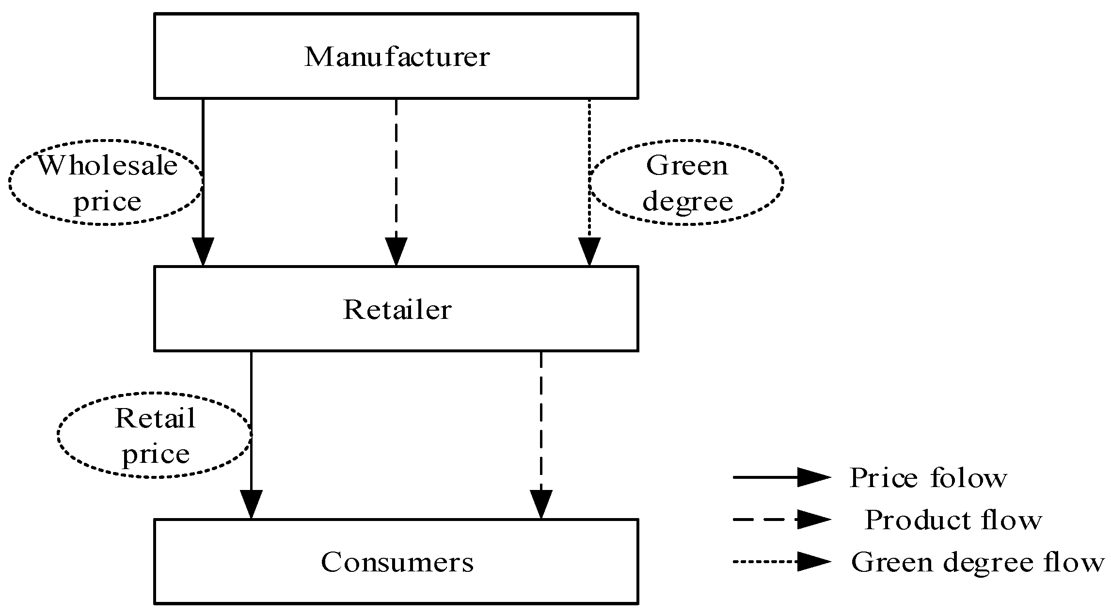
The consumers’ environmental awareness compels the manufacturer to manufacture the green products by investing heavily in new equipment or technology. Incurred investment cost in greening products leads to decreasing the manufacturer’ profit in the short term such that the manufacturer lacks motivation to produce green products. This results in two questions: Are the manufacturer’ incentive for manufacturing green products aligned? What incentive scheme can boost the manufacturer to manufacture green products? To address the two questions, in this section, the retailer offers the incentive scheme—a greening cost-sharing contract that the retailer is willing to share some greening cost with the manufacturer. Let
φ be denoted by the proportion of greening cost shared by that the retailer shares with the manufacturer. Then, the respective profits of the manufacturer and the retailer are shown as:
and
Since the manufacturer is loss-averse, then the manufacturer aims at pursuing the maximization of utility. The utility of the manufacturer is:
where
To analyze the impact of loss aversion on green supply chains, we restrict ourselves to the case
. In this case, the manufacturer’s utility is:
The retailer’s utility is:
We construct a Stackelberg game model, where the manufacturer plays the role of the leader and the retailer plays the role of the follower. The manufacturer and the retailer sequentially decide on wholesale price
w, green degree
e and retail price
p. Differentiating (31) with respect to
p yields:
Substituting (32) into (30) yields manufacturer’s utility:
The Hessian matrix on wholesale price
w and green degree
e is:
The Hessian matrix is negative definite if
i.e.,
Thus, wholesale price
and green degree
are shown, respectively:
From (32), (35), and (36), it follows that retail price is:
Thus, the manufacturer’s profit, retailer’s profit and the profit of the entire green supply chain are written, respectively:
where
, and
Proposition 5. For the green supply chain with a loss-averse manufacturer and a greening cost-sharing contract, the optimal proportion of greening cost shared by retailer shares with manufacturer is:
Proposition 6. For the green supply chain with a loss-averse manufacturer and a greening cost-sharing contract, if the probability of breakdown about bargaining game tends to zero (i.e., δ → 1), then we distinguish two cases:
Case (i) . Then, .
Case (ii) . Then, there are three subcases:
Subcase (i) if .
Subcase (ii) if .
Subcase (iii) if .
Remark 5. Proposition 5 shows that the retailer shares the optimal proportion of greening cost with the loss-averse manufacturer. Based on Proposition 6, when the probability of breakdown about the bargaining game tends to zero, if the green efficiency coefficient is high (i.e., ), then the optimal proportion of greening cost that the retailer shares with the loss-averse manufacturer is lower than the optimal proportion of greening cost that the retailer shares with a risk-neutral manufacturer. When the green efficiency coefficient is high, the consumers prefer to purchase green products because of the consumer environmental awareness. In this case, green degree has a critical impact on demand of products. Retail price and green degree in DDS-LAM are lower than those in the DSS (see Propositions 2 and 3), which implies that the retailer prefers to share a low proportion of greening cost with a loss-averse manufacturer compared to the case in which the manufacturer is risk-neutral. On the other hand, for the case where the green efficiency coefficient is low (i.e., ), if the loss-aversion coefficient of the manufacturer is sufficiently high (low), then the proportion of greening cost shared by the retailer is higher (lower) than the proportion that the retailer shares with a risk-neutral manufacturer. In this case, green degree has little effect on demand of products. If the loss-aversion level of the manufacturer is sufficiently high, to encourage the manufacturer to produce green products, the retailer is willing to share a high proportion of greening cost with a loss-averse manufacturer. If the loss-aversion level of the manufacturer is sufficiently low, then the retailer prefers to share a low proportion of greening cost with a loss-averse manufacturer since loss aversion hurts retailer’s profit.
5. Numerical Analysis
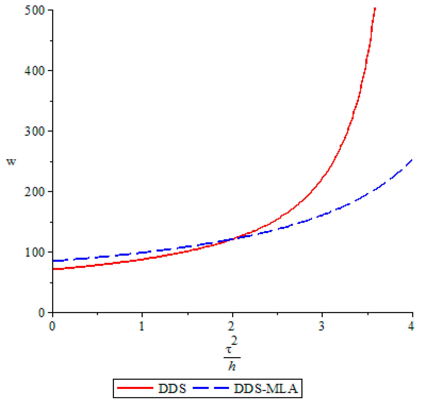
To show the impact of loss-aversion coefficient and the green efficiency coefficient on wholesale price, numerical examples are used, where a = 120, c = 20, λm = 2, and δ = 0.4.
Figure 2 presents the changes of wholesale price with the green efficiency coefficient in the two decision-making settings (i.e., DDS and DDS-LAM). In
Figure 2, if 0 <
τ2/
h < 2, then wholesale price in DDS is lower than that in DDS-MLA. In
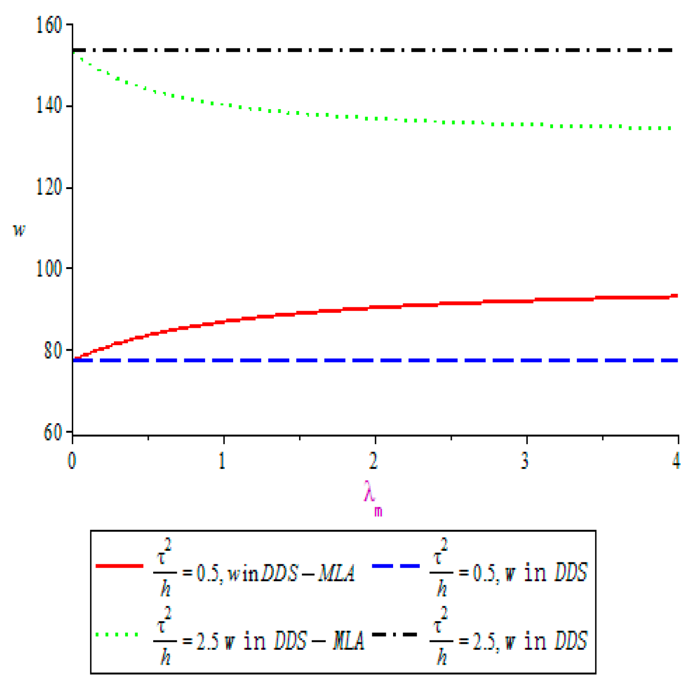
Figure 3, if
τ2/
h = 0.5, then wholesale price in DSS-MLA is increasing in
λm and is higher than that in DSS. That is, the loss-averse manufacturer sells products at a high wholesale price if the green efficiency coefficient of products is sufficiently low, since a low green efficiency coefficient of products cannot result in a significant increase in market demand, which causes the loss-averse manufacturer to sell products at a high wholesale price to obtain profit, and a higher loss aversion leads to a higher wholesale price.. If 2 <
τ2/
h < 4, then wholesale price in the DDS is higher than that in DDS-MLA. In
Figure 3, if
τ2/
h = 2.5, then wholesale price in DSS-MLA is decreasing in
λm and is lower than that in DSS. That is, the loss-averse manufacturer sells products at a low wholesale price if the green efficiency coefficient of products is sufficiently high, since a high green efficiency coefficient of products results in a significant increase in market demand, which causes the loss-averse manufacturer to sell products at a high wholesale price to obtain profit. In this case, the risk-neutral retailer sells products at a low, but the risk-neutral retailer obtains a large profit by quick turnover, which causes the loss-averse manufacturer to sell products at a low wholesale price to obtain profit, and a higher loss aversion leads to a lower wholesale price. If
τ2/
h = 2, wholesale price has no difference in the two decision-making settings. In addition, wholesale price increases with the green efficiency coefficient of products
τ2/
h.
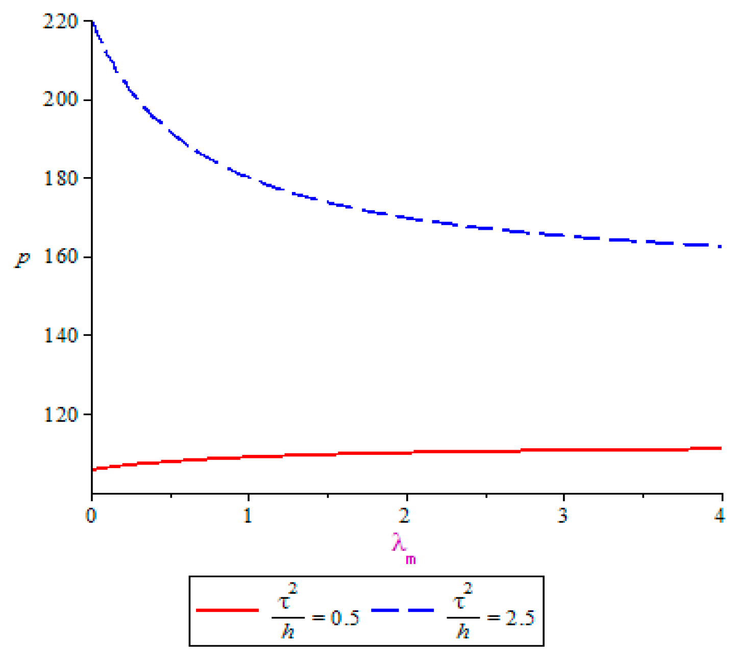
We use numerical examples to analyze retail price with respect to the loss-aversion coefficient and the green efficiency coefficient. Let a = 120, c = 20, λm = 2, and δ = 0.4.
In
Figure 4, if 0 <
τ2/
h < 1, then retail price in CDS is lower than that in DDS, while the latter is lower than retail price in DDS-LAM. If 1 <
τ2/
h < 2, then retail price in the CDS is higher than that in DDS, while the latter is higher than retail price in DDS-LAM. If
τ2/
h = 1, retail price has no difference in the three decision-making settings. In addition, retail price in the three decision-making settings increases with the green efficiency coefficient of products
τ2/
h. The green efficiency coefficient has an important impact on retail price. In
Figure 5, if
τ2/
h = 0.5, then retail price in DSS-MLA is increasing in
λm. If
τ2/
h = 2.5, then retail price in DSS-MLA is decreasing in
λm. From
Figure 3 and
Figure 5, it follows that wholesale price and retail price increase with
λm if the green efficiency coefficient of products is at a lower level (i.e.,
τ2/
h = 0.5), while wholesale price and retail price decrease with
λm if the green efficiency coefficient of products is at a higher level (i.e.,
τ2/
h = 2.5). In other words, for the case where the green efficiency coefficient of products is lower (i.e., the consumer sensitivity to green improvements is lower or the cost coefficient of green degree per unit is higher), the manufacturer with loss aversion can make up for the cost incurred (i.e., losses), which is used to invest in the new equipment or technology, by increasing wholesale price. On the other hand, the retailer increases retail price to improve his profit, since lower sensitivity to green degree leads to a lower market demand for green products. For the case where the green efficiency coefficient of products is higher (i.e., the consumer sensitivity to green improvements is higher or the cost coefficient of green degree per unit is lower), a higher level of consumer sensitivity to green improvements leads to increasing heavily market demand for green products. The manufacturer with loss aversion decreases wholesale price to increase sales such that the manufacturer improves his profit, while the retailer decreases retail price to sell more products such that the retailer increases his profit.
To explore the impact of the loss-aversion coefficient and the green efficiency coefficient on green degree, numerical examples are used, where a = 120, c = 20, λm = 2, and δ = 0.4.
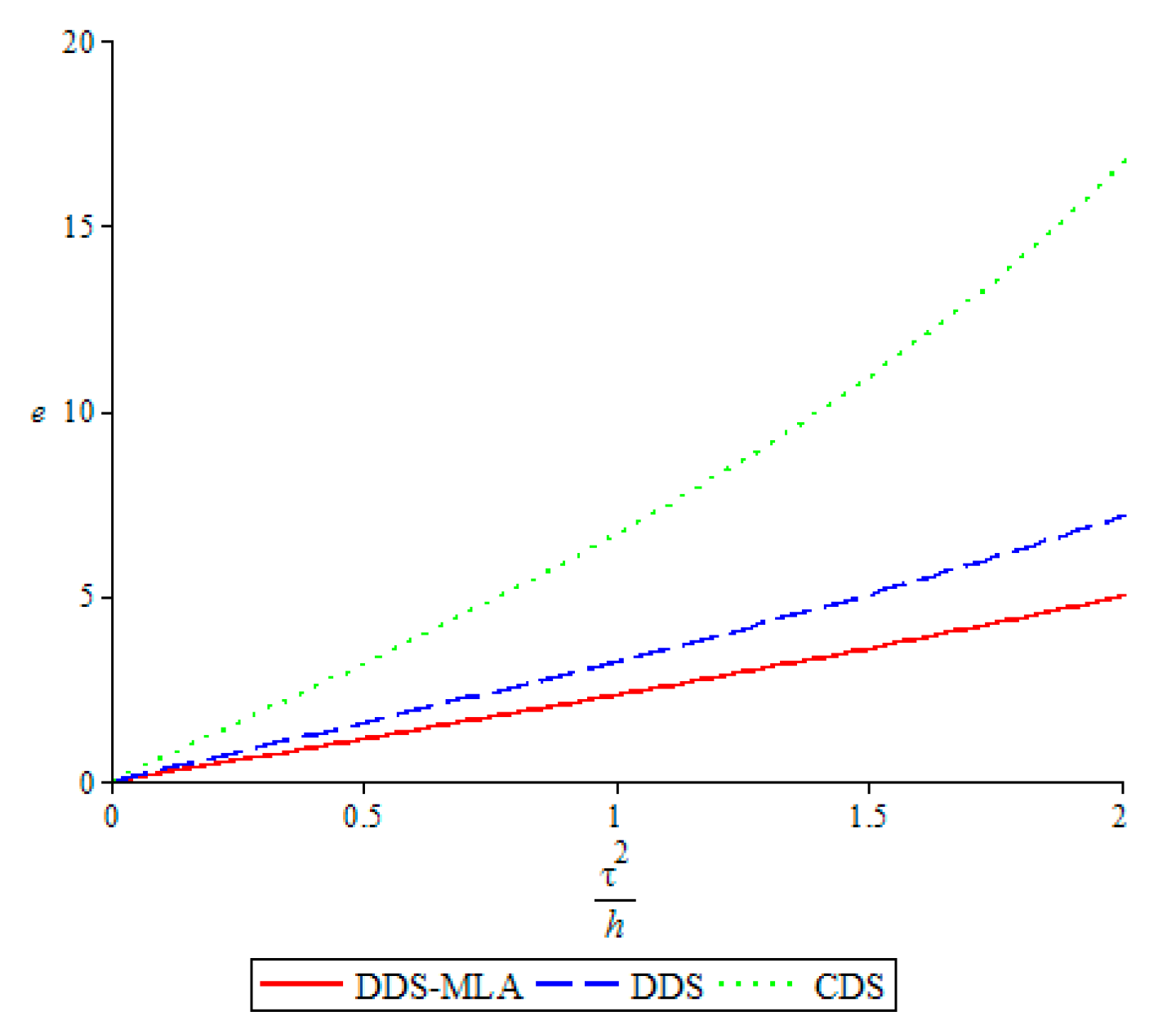
In
Figure 6, green degree in the three decision-making settings increases with the green efficiency coefficient of products
τ2/
h. Green degree in CDS is the highest in the three decision-making settings, while green degree in DDS-LAM is the lowest in the three decision-making settings. Furthermore, green degree in the three decision-making settings increases with
τ2/
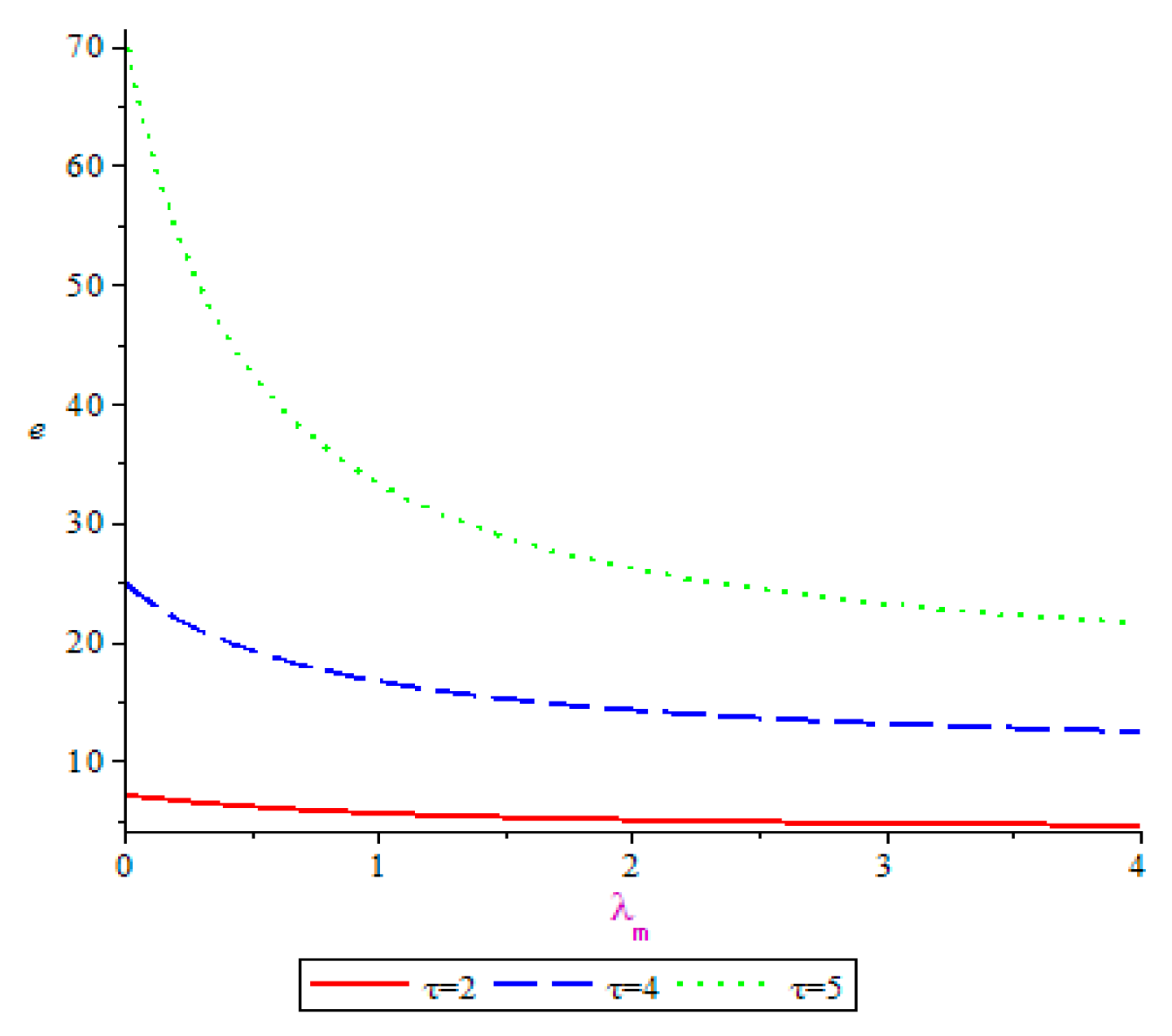
h. Green degree in CDS is the highest in the three decision-making settings, while green degree in DDS-LAM is the lowest. The change of green degree with the loss-aversion coefficient is shown in
Figure 7. A higher level of consumer sensitivity to green improvements leads to increasing heavily market demand for green products. Thus, the manufacturer is more motivated to invest in new equipment or technology to produce green products such that the manufacturer increases his profit. On the other hand, green degree decreases with the loss-aversion coefficient
λm. The manufacturer with loss aversion pays more attention to gains or losses than to profits. Investing in new equipment or technology decreases the manufacturer’s profit. Thus, the higher the manufacturer’s degree of loss aversion is, the lower the probability of producing green products is. This implies that a higher level of loss aversion leads to a lower green degree of products.
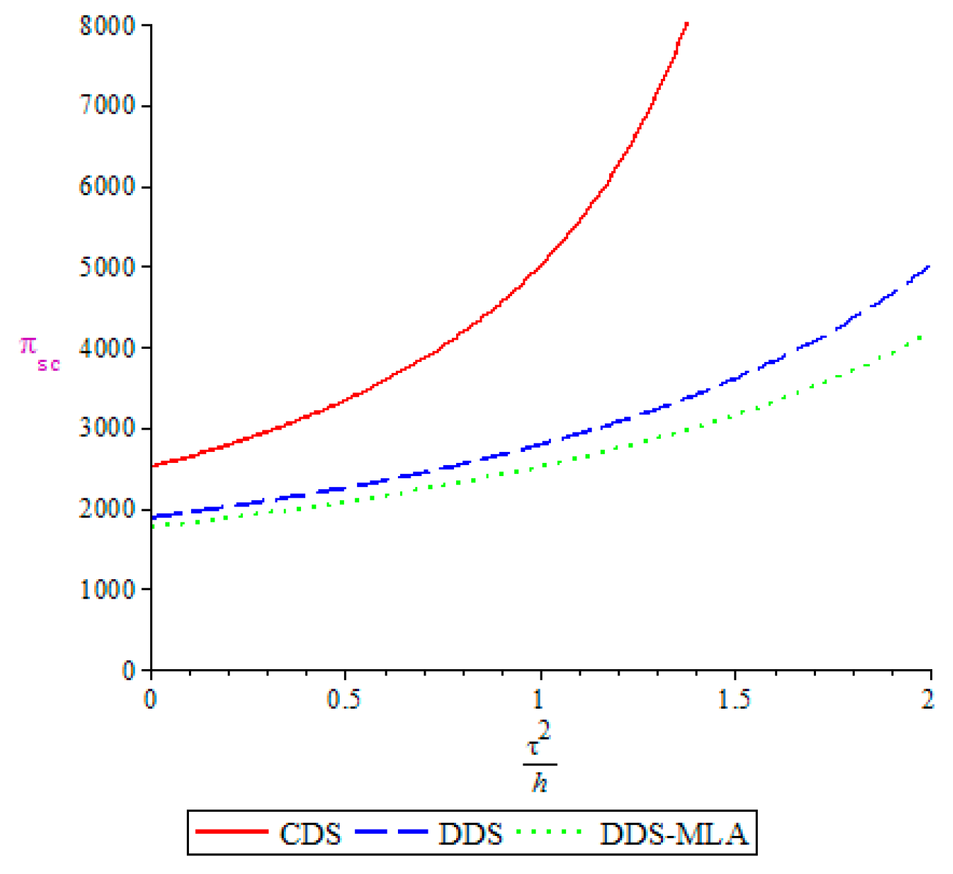
Figure 8 shows the changes of with the profit of green supply chain with green efficiency coefficient.
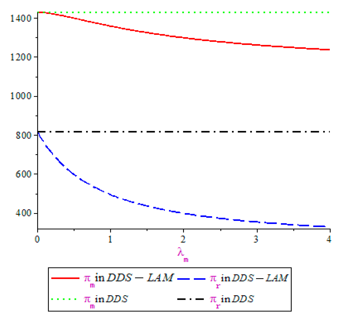
Figure 9 shows the changes of profits of manufacturer and retailer with loss-aversion coefficient. In
Figure 8, the profit of the entire green supply chain in CDS is higher than that in DDS, while the latter is higher than the profit of the entire green supply chain in DDS-LAM. Note that the profit of the entire green supply chain in the three decision-making settings increases with
τ2/
h. The profit of the entire green supply chain in CDS is the highest in the three decision-making settings, while the profit of the entire green supply chain in DDS-LAM is the lowest. In other words, the efficiency of the green supply chain in CDS (DDS-LAM) is the highest (lowest) in the three decision-making settings. In
Figure 9, manufacturer’s profit in DDS-LAM is lower than that in DDS. A similar conclusion holds for the retailer. In addition, manufacturer’s profit and retailer’s profit decrease with manufacturer’s levels of loss aversion. This implies that a loss-averse manufacturer is willing to sacrifice part of his own profit and take actions to punish the retailer such that the manufacturer maintain the gains relative to the reference point.
To explore the impact of the proportion of greening cost shared by the retailer on profits of manufacturer and retailer, numerical examples are used, where
a = 120,
c = 20,
λm = 2,
δ = 0.4,
h = 4, and
τ = 10. In
Figure 10, after executing a greening cost-sharing contract, the profits of manufacturer and retailer are first increasing and then decreasing with φ. From
Figure 10, it follows that executing the greening cost-sharing contract can improve the profits of manufacturer and retailer if an appropriate proportion of greening cost is shared by the retailer. That is, a greening cost-sharing contract can boost the manufacturer to manufacture green products if the retailer shares an appropriate proportion of greening cost with the manufacturer.
6. Summary
6.1. Managerial Insights
This study can be applied to the green supply chain where the manufacturer occupies an absolute dominant position in the green supply chain. For example, the mobile phone industry supply chain includes HUAWEI, APPLE, and SAMSUNG. The model constructed in this paper helps non-rational decision-makers to make the optimal decisions in the green supply chains. In particular, in this paper, the model helps the loss-aversion manufacturer to make the optimal wholesale price decision and the optimal green degree decision. In addition, the model helps the risk-neutral retailer to make the optimal retail price decision. Thus, our model is of important theoretical and practical significance. On the one hand, this model promotes further theoretical study of green supply chains by considering a two-echelon green supply chain with a manufacturer and a retailer, where the manufacturer is loss-averse and the retailer is risk-neutral. On the other hand, this model helps the loss-aversion manufacturer and the risk-neutral retailer to make the optimal decisions in the green supply chains by providing some useful managerial insights into how to make pricing, green degree and coordination decisions. First, if the green efficiency coefficient of products is sufficiently low, then the risk-neutral retailer prefers to make a high retail price and the loss-aversion manufacturer sells products at a high wholesale price, since in the green supply chains market demand depends on retail price and green degree of products and a lower green efficiency coefficient of products cannot result in a significant increase in market demand, which makes the risk-neutral retailer and the loss-aversion manufacturer set a high retail price and a high wholesale price to obtain profits, respectively. In addition, if the green efficiency coefficient of products is sufficiently high, then the risk-neutral retailer prefers to make a low retail price and the loss-aversion manufacturer sells products at a low wholesale price, since a higher level of environmental awareness causes consumers to purchase higher-green-degree products when the green efficiency coefficient of products is sufficiently high, which results in dramatically increasing market demand. In this case, the risk-neutral retailer sells products at a low price, but the risk-neutral retailer obtains a large profit by quick turnover, which causes the loss-averse manufacturer sells products at a low wholesale price. Second, the loss-aversion manufacturer will make a low green degree, since the manufacturer with loss aversion is not willing to invest in new equipment or technology to produce the green products. Finally, a greening cost-sharing contract can improve the efficiency of green supply chain if the retailer shares an appropriate proportion of greening cost with the manufacturer. In this case, executing a greening cost-sharing contract can improve the profits of the loss-aversion manufacturer and the risk-neutral retailer, which results in the loss-aversion manufacturer and the risk-neutral retailer preferring to execute the greening cost-sharing contract. It is worthwhile to note that members of green supply chains have to consider the green efficiency coefficient of products to apply our model, since the green efficiency coefficient of products has an important impact on the optimal wholesale price decision, the optimal green degree decision, and the retail price decision.
6.2. Concluding Remarks
In this paper, the manufacturer’s behavioral preference of loss aversion is formalized by Shalev’s model of loss aversion, where the subgame perfect equilibrium partition is regarded as a reference point of loss aversion. We investigate the impacts of loss aversion and green efficiency coefficient on retail price, wholesale price, green degree, profits of members, and the profit of the entire green supply chain under three decision-making settings (i.e., the CDS, DDS, and DDS-LAM). Furthermore, to achieve coordination of green supply chain with a loss-averse manufacturer and a risk-neutral retailer, we discuss the greening cost-sharing contract.
The green efficiency coefficient has an important effect on wholesale price, retail price and green degree. The manufacturer’s loss aversion leads to a low wholesale price if the green efficiency coefficient is sufficiently high, or wholesale price in DDS-LAM is not less than that in DDS. If the green efficiency coefficient is sufficiently high, then retail price in CDS is higher than that in DDS, which is a reversed result of the traditional supply chains. The manufacturer’s loss aversion further decreases retail price, which means that retail price is the lowest in DDS-LAM, followed by DDS, while it is the highest in CDS. When it comes to the green degree, the green degree is the lowest in DDS-LAM, followed by DDS, while it is the highest in CDS regardless of the green efficiency coefficient. In addition, wholesale price and retail price decrease (increase) with the manufacturer’s level of loss aversion if the green efficiency coefficient is sufficiently high (low) and green degree decreases with the manufacturer’s level of loss aversion, as shown in numerical analysis.
Moreover, for the manufacturer, the manufacturer’s loss aversion leads to the low profit. Compared with the risk-neutral manufacturer, the manufacturer is hurt by his own loss aversion. For retailer, the profit in DDS-LAM is lower than that in DDS. Retailer is also hurt by the manufacturer’s loss aversion. These further decrease the profit of the green supply chain. Thus, the profit of the entire green supply chain is the highest in CDS, followed by DDS, while it is the lowest in DDS-LAM. In addition, in DDS-LAM, profits of chain members decrease with the manufacturer’s level of loss aversion, as shown in numerical analysis.
Finally, the coordination of the green supply chain with a loss-averse manufacturer and a risk-neutral retailer can be achievable by executing a green cost-sharing contract if the retailer shares an appropriate proportion with the loss-averse manufacturer.
This paper considers a green supply chain with a loss-averse manufacturer and a risk-neutral retailer. It is interesting to extend our study to incorporate the governmental interventions, since facing with the deteriorating environment governments pay increasing attention to environmental issues and promulgate a series of policy on environmental protection, especially the environmental awareness of enterprises. Moreover, considering the impact of loss aversion in the competition among multiple manufacturers or multiple retailers would be another rewarding issue.


