An Approach of Trustworthy Measurement Allocation Based on Sub-Attributes of Software

Abstract

Measurement of software trustworthiness is an important research field in the software engineering, which is very useful for analyzing the software quality. In this paper, we propose a mathematical programming approach to allocate the trustworthy degree to each sub-attribute of some software attribute appropriately and then to make the trustworthy degree of this attribute maximize under some constraint conditions. Some sufficient or necessary conditions for analyzing this mathematical programming problem are investigated. Moreover, a polynomial allocation algorithm is given for computing the optimal solution of this mathematical programming. Finally, an example is given in order to show the significance of this work. The results obtained here are useful for improving the software quality by adjusting the trustworthy degree of each sub-attribute under the same cost.

1. Introduction

Due to the increasing dependence on software, people pay more and more attention to the research into software trustworthiness. One of the core scientific problems in this research is the software trustworthiness measurement [1]. Software trustworthiness measurement is the quantification of software trustworthiness, which can provide evidence for increasing the trustworthiness of the implementation of software. The software trustworthiness can be characterized by many attributes [2,3,4,5], which are called trustworthy attributes in this paper. Trustworthy attributes are separated into critical attributes and non-critical attributes [6]. Critical attributes are the attributes that trustworthy software must have and the other trustworthy attributes are referred to as non-critical attributes [6]. Trustworthy attributes are normally at too high of a level to be measurable directly; hence, they are further subdivided into sub-attributes. Many software trustworthiness measurement models based on the decompositions of trustworthy attributes are proposed. Typical ones include ISO/IEC 25010: 2011 [7], classification model [8], Bayesian networks [9], weakness analysis [10], questionnaires and statistical analysis [11,12], evidence theory [13], dynamic statistical analysis [14], data mining [15], fuzzy theory [16], rough set theory [17], and user feedback [18]. Weights of different attributes play key roles in obtaining accurate trustworthiness measurement; Ref. [19] proposes an approach for determining weights based on the subjective and objective integration; it gets the subjective weights by aggregating the positive reciprocal matrices given by the evaluations of different experts and acquires objective weights based on the trustworthy degrees of the attributes and the subjective weights. However, few researchers pay attention to using more rigorous approaches to software trustworthiness measurement. In order to make the software trustworthiness measure more rigorous, axiomatic approaches are applied to measure software trustworthiness by us [6,20,21,22,23,24].

The software trustworthiness measurement approach describes the procedure of determining the trustworthy degree of a software program with given trustworthy degrees of attributes. The allocation of software trustworthiness, which determines degrees of trustworthy attributes with given trustworthy degree of a software program, is very important too. It is useful for improving the software trustworthiness by adjusting the degree of each trustworthy attribute under the same cost. Ma et al. [25] have investigated the reverse of the software trustworthiness measurement approach proposed in [24]. However, as we mentioned above, trustworthy attributes are normally at too high a level to be measurable directly, and they are further subdivided into sub-attributes. In this paper, based on the trustworthy attribute measurement model built in [24], we deal with the problem of how to determine trustworthy degrees of sub-attributes with given trustworthy degree of a trustworthy attribute. We build a mathematical programming (MP) model to allocate the trustworthy degree of a trustworthy attribute to its sub-attributes appropriately, and discuss some sufficient or necessary conditions for analyzing this MP. Moreover, an allocation algorithm is proposed for solving this MP. Finally, a concrete example is presented in order to state the significance of our work. The results obtained here are useful for guiding and controlling the software quality by adjusting the trustworthy degree of each sub-attribute under the same cost.

The rest of the paper is organized as follows. In Section 2, we describe the trustworthy attribute measurement model proposed in [24]. An allocation model for software attribute trustworthiness defined as a mathematical programming model MP is introduced in Section 3 and some sufficient or necessary conditions for analyzing this MP are also discussed in this section. An allocation algorithm for solving the MP built in Section 3 is given in Section 4 and an example is presented in Section 5. The conclusions and future works are presented in the last section.

2. Software Attribute Trustworthiness Measurement Model

Axiomatic approaches formalize the empirical understandings of software attributes by the definitions of desirable measure properties [26,27,28]. They can provide precise and formal terms for the quantification of software attributes. We once used the axiomatic approaches to measure software trustworthiness based on attributes. Four desirable properties of the software trustworthiness measurement based on attributes were first given by us in [6], that is, monotonicity, acceleration, sensitivity and substitutivity. Considering the software trustworthiness related to user expectation, we putted forward the expectability property in [21]. We further improved the above property set and added three new properties: non-negativity, nullability and appropriateness of the ratio of trustworthy attributes [23]. In Ref. [22], we extended the above works to apply axiomatic approaches to measure software trustworthiness based on the decompositions of trustworthy attributes, proposed the desirable measure properties in the view of the decompositions of trustworthy attributes, established a software trustworthiness measurement model based on the decompositions of attributes as described in Definition 1, and validated this model from the theory by proving that it complied with the properties given in [22].

Definition 1

(Software trustworthiness measurement model established in [22]).

$$T={\{\alpha {[{(\frac{y_{min}}{10})}^{ϵ}{y}_1^{{\alpha }_1}{y}_2^{{\alpha }_2}\cdots y_m^{{\alpha }_m}]}^{-\rho }+\beta {[y_{m+1}^{{\beta }_{m+1}}{y}_{m+2}^{{\beta }_{m+2}}\cdots y_{m+s}^{{\beta }_{m+s}}]}^{-\rho }\}}^{-\frac{1}{\rho }},$$

where

1.

$y_1,\cdots ,y_m$ are the trustworthy degrees of critical attributes and $y_{m+1},\cdots ,y_{m+s}$ are the trustworthy degrees of non-critical attributes;

2.

T is the software trustworthiness measure function regarding $y_1,\cdots ,y_{m+s}$;

3.

α and β are used to distinguish the contributions of critical attributes and non-critical attributes to the software trustworthiness, which satisfy that $\alpha +\beta =1$, ${\alpha }_1,\cdots ,{\alpha }_m$ are the weight values of critical attributes and ${\beta }_{m+1},\cdots ,{\beta }_{m+1}$ express the relative importance of the non-critical attributes;

4.

ϵ is used to control the effect of the minimum critical attribute on the software trustworthiness;

5.

$0<\rho$ is a parameter related to the substitutivity between critical and non-critical attributes;

The benefits of using the exponential model rather than the model of linear combination (i.e., $y={\sum }_{j=1}^n{\alpha }_i{y}_i$) for computing the trustworthy degree have been stressed in [20] in detail.

The spacecraft software trustworthiness is one of the key factors to ensure the space mission’s success. However, the evaluation of spacecraft software trustworthiness is only qualitative heretofore. In order to make the spacecraft software trustworthiness measurement more rigorous, axiomatic approaches are used to measure spacecraft software trustworthiness based on the decompositions of trustworthy attributes by us [24]. The trustworthy degree of spacecraft software is obtained by aggregating the trustworthy degree of each attribute; furthermore, the trustworthy degree of each attribute is computed by using the trustworthy degrees of its sub-attributes. Considering the particularities of spacecraft softwares, we think that all of their trustworthy attributes are critical and let $ϵ=0$; then, the measurement model given in Definition 1 is simplified, as shown in Definition 2 [24].

Definition 2

(Simplified software trustworthiness measurement model used in [24]).

$$T=y_1^{{\alpha }_1}{y}_2^{{\alpha }_2}\cdots y_n^{{\alpha }_n},$$

where

1.

$y_1,\cdots ,y_n$ are the trustworthy degrees of trustworthy attributes and ${\alpha }_1,\cdots ,{\alpha }_n$ are their weight values;

2.

T is the software trustworthiness measure function regarding $y_1,\cdots ,y_n$.

The simplified software trustworthiness measurement model not only satisfies the set of properties given in [22] but also is in agreement with the idea of Cannikin Law. In Ref. [24], the trustworthy attribute measurement model uses the same computational model as the software trustworthiness measurement model described in Definition 2, which is depicted in Definition 3 [24].

Definition 3

(Software attribute trustworthiness measurement model given in [24]).

$$y=\prod _{j=1}^n{x}_{{}_j}^{{\alpha }_j},$$

where

1.

y is the trustworthy degree of some attribute;

2.

n is the number of trustworthy sub-attributes that comprises this trustworthy attribute;

3.

$x_j\in \{t_1,t_2\cdots ,t_k\}$ is the trustworthy degree of the j-th sub-attribute of this trustworthy attribute, $t_i(1\le i\le k)$ are the trustworthy levels of sub-attributes with $t_1>t_2>\cdots >t_k$ and take values from the set $\{1,0.9,0.8,0.7,0.6,0.5,0.4,0.3,0.2,0.1\}$;

4.

${\alpha }_j$ is the weight value of the j-th sub-attribute, with ${\sum }_{j=1}^n{\alpha }_j=1,0\le {\alpha }_n\le {\alpha }_{n-1}\le \cdots \le {\alpha }_1\le 1$.

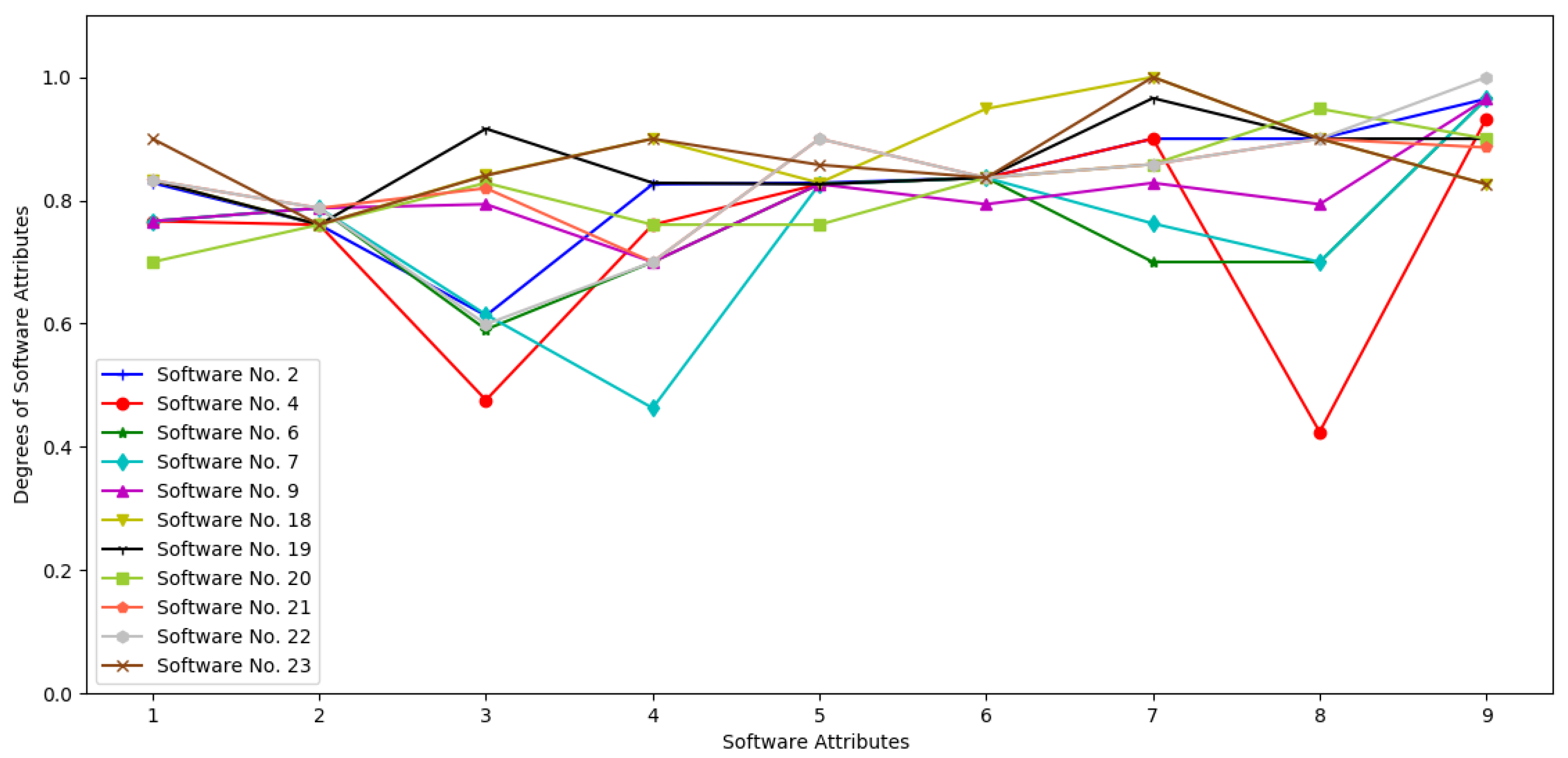
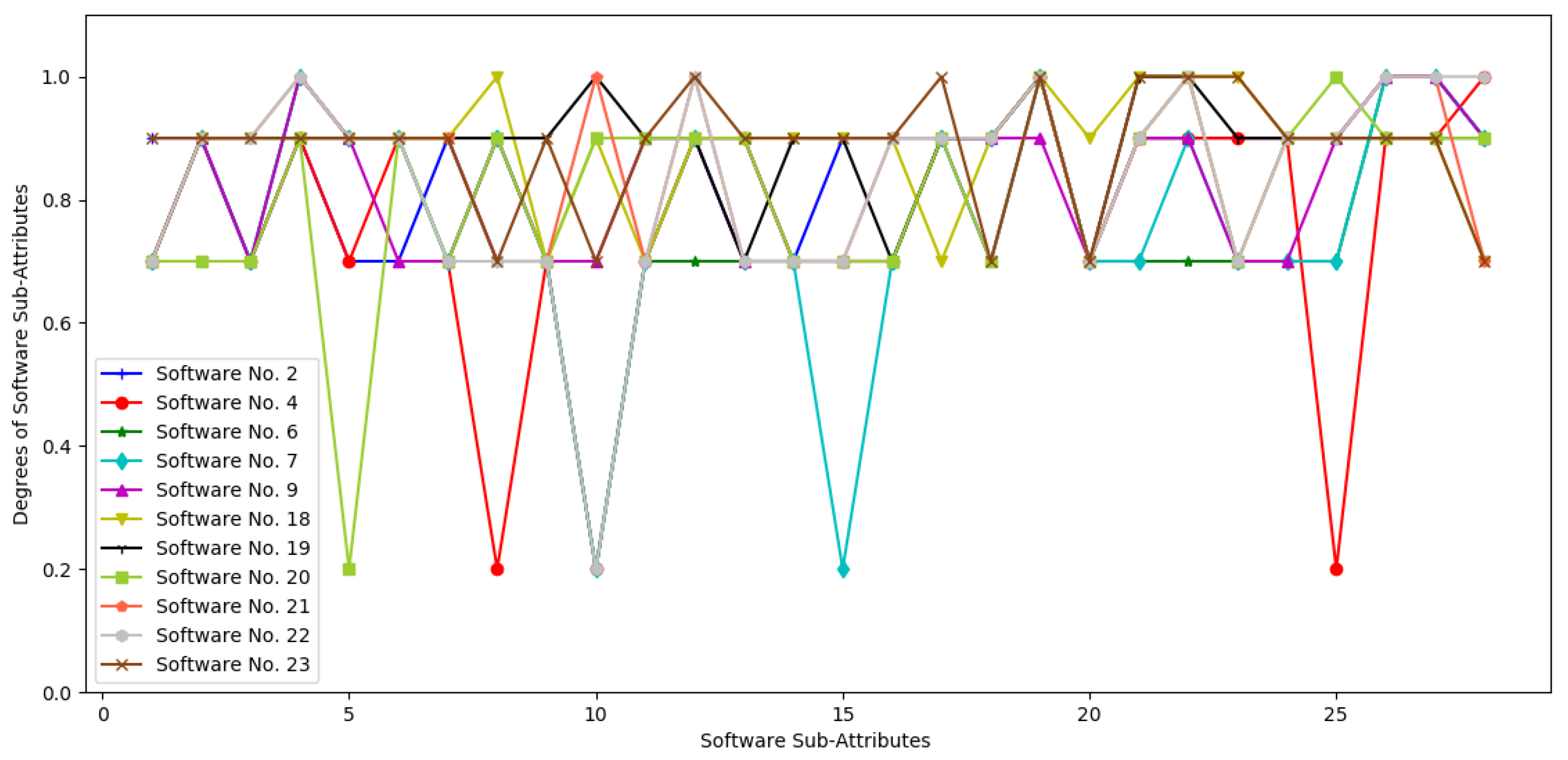
Meanwhile, an empirical validation is carried out by applying the measurement models given in Definitions 2 and 3 to measure 23 spacecraft software programs [24]. The critical attributes of spacecraft software are composed of nine attributes and these nine attributes consist of 28 sub-attributes. The expert panel that consists of 10 experts grade the 28 sub-attributes and finally measure the trustworthiness of the 23 spacecraft softwares from bottom to up. The distributions of trustworthy degrees of software attributes and sub-attributes of 11 representative software programs are shown in Figure 1 and Figure 2, respectively. The trustworthy degrees of software attributes and sub-attributes are consistent with the actual situations of software product development [24], which truly reflect the spacecraft software attribute and sub-attribute trustworthiness. On the one hand, from Figure 1 and Figure 2, we can easily find the weak links in the progress of software development [24]. Therefore, the measurement models described in Definitions 2 and 3 are reasonable and effective.

Ma et al. [25] have studied the allocation of software trustworthiness based on the software trustworthiness measurement model presented in Definition 2. Since the ranges of the free variables of the software trustworthiness measurement model given in Definition 2 are different from that of the software attribute trustworthiness measurement model described in Definition 3, the allocation approach of software trustworthiness proposed in [25] is not suitable for the allocation of software attribute trustworthiness.

3. Allocation Model for Software Attribute Trustworthiness

According to the trustworthy attribute measurement model described in Definition 2, we define an allocation model for software attribute trustworthiness as the following mathematical programming model.

Definition 4

(Allocation Model for Software Attribute Trustworthiness).

Mathematical Programming (MP)

$$y=max\prod _{j=1}^n{x}_{{}_j}^{{\alpha }_j},$$

Subject to:

$$\left\{\begin{array}{c}{x}_j\in A=\{t_1,t_2\cdots ,t_k\},j=1,2,\cdots ,n,\hfill \\ min\sum _{j=1}^n{x}_j,\hfill \\ y\ge t,\hfill \end{array}\right.$$

(1)

where

1.

y is the trustworthy degree of some attribute;

2.

n is the number of trustworthy sub-attributes that comprise this trustworthy attribute;

3.

$x_j$ is the trustworthy degree of the $j-th$ sub-attribute of this trustworthy attribute;

4.

${\alpha }_j$ is the weight value of the $j-th$ sub-attribute such that ${\sum }_{j=1}^n{\alpha }_j=1$ and $0\le {\alpha }_n\le {\alpha }_{n-1}\le \cdots \le {\alpha }_1\le 1$;

5.

$t_i(1\le i\le k)$ are the trustworthy levels of the sub-attributes with $t_1>t_2>\cdots >t_k$, and take values from the set $\{1,0.9,0.8,0.7,0.6,0.5,0.4,0.3,0.2,0.1\}$;

6.

t is the specified trustworthy degree that this attribute must reach with $0\le t\le 1$.

The main differences between the allocation of software attribute trustworthiness and the allocation of software trustworthiness proposed in [25] are as follows. The allocation of software trustworthiness describes the process of determining the trustworthy degree of each software attribute with the given trustworthy degree of a software [25], the range of each attribute value is [0,1]. The allocation of software attribute trustworthiness describes the process of determining the trustworthy degree of each software sub-attribute according to the given software attribute trustworthiness, the trustworthy degrees of the sub-attributes come from the set $\{1,0.9,0.8,0.7,0.6,0.5,0.4,0.3,0.2,0.1\}$. Moreover, the allocation model given in [25] only requires finding the feasible solution of the allocation of software trustworthiness; however, the allocation model created above requires finding the optimal solution of the allocation of software attribute trustworthiness.

Proposition 1.

Let $y={\prod }_{i=1}^n{x}_i^{{\alpha }_i}$, ${\alpha }_{j-1}\ge {\alpha }_j(j=2,3,\cdots ,n)$ and $x_{j-1}\ge x_j>0(j=2,\cdots ,n)$, i.e., $x_j$ is monotonic non-increasing with respect to the subscript j. Then, y will be non-increasing when we exchange any $x_i$ and $x_j$ such that $i<j$. That is, suppose that

$$y^{\prime }=x_1^{{\alpha }_1}\cdots x_{i-1}^{{\alpha }_{i-1}}{x}_j^{{\alpha }_i}{x}_{i+1}^{{\alpha }_{i+1}}\cdots x_{j-1}^{{\alpha }_{j-1}}{x}_i^{{\alpha }_j}{x}_{j+1}^{{\alpha }_{j+1}}\cdots x_n^{{\alpha }_n}.$$

Then, $y\ge y^{\prime }$.

Proof. 

$$\begin{array}{ccc}\frac{y}{y^{\prime }}\hfill & =\hfill & \frac{x_i^{{\alpha }_i}{x}_j^{{\alpha }_j}}{x_j^{{\alpha }_i}{x}_i^{{\alpha }_j}}\hfill \\ & =\hfill & {(\frac{x_i}{x_j})}^{{\alpha }_i}{(\frac{x_j}{x_i})}^{{\alpha }_j}\hfill \\ & =\hfill & {(\frac{x_i}{x_j})}^{{\alpha }_i-{\alpha }_j}\hfill \\ & \ge 1\hfill & (\mathrm{since}{x}_i\ge x_j\mathrm{and}{\alpha }_i\ge {\alpha }_j).\hfill \end{array}$$

Hence, $y\ge y^{\prime }$. □

This proposition shows that the value of y is non-decreasing when the trustworthy degree assigned to $x_i$ satisfies the least subscript i, the largest value of $x_i$. Furthermore, we have the following corollary.

Corollary 1.

(1) Let $y={\prod }_{j=1}^n{(t_k+{\delta }_j)}^{{\alpha }_j}$, where ${\alpha }_{j-1}\ge {\alpha }_j$ and ${\delta }_{j-1}\ge {\delta }_j$ for any $j=2,3\cdots ,n$. Then, y will be non-increasing when we exchange ${\delta }_i$ and ${\delta }_j$ in y for any $i<j$. (2) Given an assignment set $\{a_1,\cdots ,a_n\}$ for $x_j(j=1,\cdots ,n)$ in $y={\prod }_{j=1}^n{x}_j^{{\alpha }_j}$, where ${\alpha }_{j-1}\ge {\alpha }_j$ for any $j=2,3\cdots ,n$, and then y takes maximal value if and only if the assignments satisfy the least subscript j, the largest assignment of $x_j$.

Corollary 1 will be useful for the latter algorithm that allocates a trustworthy degree to each sub-attribute. Now, we give an example.

Example 1.

Let

$$y=x_1^{0.4}{x}_2^{0.2}{x}_3^{0.19}{x}_4^{0.11}{x}_5^{0.1}$$

and $\{0.1,0.1,0.2,0.6,1\}$ be an assignment set for $x_j(j=1,\cdots ,5)$. Then, some different assignments of $x_j$ exist, for example, $(x_1,x_2,x_3,x_4,x_5)=(0.6,0.2,0.1,1,0.1)$. Among them, the assignment $(x_1,x_2,x_3,x_4,x_5)=(1,0.6,0.2,0.1,0.1)$ will make y maximize.

However, it should be pointed out that the maximal value of y is affected by the weights even if ${\sum }_{j=1}^n{x}_j$ keeps unchanged, which is witnessed by the following example.

Example 2.

Let

$$\begin{array}{ccc}y\hfill & =\hfill & x_1^{0.4}{x}_2^{0.2}{x}_3^{0.19}{x}_4^{0.11}{x}_5^{0.1},\hfill \\ \overline{y}\hfill & =\hfill & x_1^{0.5}{x}_2^{0.3}{x}_3^{0.1}{x}_4^{0.06}{x}_5^{0.04},\hfill \end{array}$$

and take $(x_1,x_2,x_3,x_4,x_5)=(1,0.6,0.2,0.1,0.1)$ and $(1,0.4,0.4,0.1,0.1)$, respectively. Obviously, $x_j$ is monotonic non-increasing with respect to the subscript j and ${\sum }_{j=1}^5{x}_j=2$ in both cases. However, it is easy to see that $y(1,0.6,0.2,0.1,0.1)<y(1,0.4,0.4,0.1,0.1)$, but $\overline{y}(1,0.6,0.2,0.1,0.1)>\overline{y}(1,0.4,0.4,0.1,0.1)$.

This example shows that the weights, in particular, degree of proximity between weights will affect the order between y and $\overline{y}$. Hence, under the condition of ${\sum }_{j=1}^n{x}_j$ being unchanged, if there is only an assignment set, then y takes maximal value when assignments satisfy the least subscript j, the largest value of $x_j$; whereas, if there are two assignment sets, then the maximal value is taken by comparing the values of y under these two assignments such that the least subscript j, the largest value of $x_j$.

Obviously, the MP (1) has an optimal solution when $t_1=1\in A$. In this case, we can give a coarse estimate of ${\sum }_{j=1}^n{x}_j$. For this purpose, we first make a little preparation.

Lemma 1.

(Chebyshev inequality) Let $a_i,b_i\ge 0(i=1,2,\cdots ,n)$. If $a_{i-1}\le a_i$ and $b_{i-1}\le b_i$ for any $i=2,\cdots ,n$, then

$$\sum _{i=1}^n{a}_i{b}_{n-i+1}\le \frac{1}{n}(\sum _{i=1}^n{a}_i)(\sum _{i=1}^n{b}_i)\le \sum _{i=1}^n{a}_i{b}_i.$$

Lemma 2.

(Bernoulli inequality) Let $c_i\ge -1(i=1,2,\cdots ,n)$ and $c_i{c}_j\ge 0$ for any $i,j$. Then,

$$1+\sum _{i=1}^n{c}_i\le \prod _{i=1}^n(1+c_i).$$

Proposition 2.

Suppose that the MP (1) has an optimal solution. Then, ${\sum }_{j=1}^n{x}_j\ge t^n+(n-1)$ implies $y\ge t$.

Proof. 

Let $y={\prod }_{j=1}^n{x}_{{}_j}^{{\alpha }_j}$ and $a\in (0,1)$. Then,

$${log}_{a}y=\sum _{j=1}^n{\alpha }_j{log}_a{x}_j.$$

Clearly, ${log}_a{x}_j\ge 0$ for any $j=1,2,\cdots ,n$. Furthermore, the MP (1) has an optimal solution that implies that $x_{j-1}\ge x_j$ by Corollary 1 (2) and then ${log}_a{x}_{j-1}\le {log}_a{x}_j$ for any $j=2,\cdots ,n$. Hence,

$$\begin{array}{ccc}{log}_{a}y\hfill & =\hfill & \sum _{j=1}^n{\alpha }_j{log}_a{x}_j\hfill \\ & \ge \hfill & \frac{1}{n}(\sum _{j=1}^n{\alpha }_i)(\sum _{j=1}^n{log}_a{x}_j)(\mathrm{by}\mathrm{Lemma}1)\hfill \\ & =\hfill & \frac{1}{n}\sum _{j=1}^n{log}_a{x}_j\hfill \\ & =\hfill & \frac{1}{n}{log}_a\prod _{j=1}^n{x}_j.\hfill \end{array}$$

It follows that $y^n\le {\prod }_{j=1}^n{x}_j$. Furthermore, by Bernoulli inequality, we have that

$$\prod _{j=1}^n{x}_j\ge 1+\sum _{j=1}^n(x_j-1)=\sum _{j=1}^n{x}_j-(n-1).$$

Consequently, $y^n\le {\sum }_{j=1}^n{x}_j-(n-1)$. Thus, when ${\sum }_{j=1}^n{x}_j\ge t^n+(n-1)$ holds, $y\ge t$ must hold. The proof is completed. □

The significance of this proposition is that sometimes it is convenient to find the least ${\sum }_{j=1}^n{x}_j$ close to $t^n+(n-1)$.

Example 3.

$$\begin{array}{cc}\hfill MP:y=& max{x}_1^{0.35}{x}_2^{0.33}{x}_3^{0.32},\hfill \\ \hfill Subjectto:& x_j\in \{1.0,0.9,0.7\},\hfill \\ & min\sum _{j=1}^3{x}_j,\hfill \\ & y\ge 0.85\hfill \end{array}$$

Then, $t^n+(3-1)={0.85}^3+2=2.6141$. After computing, $y_{max}=0.8305$ when ${\sum }_{j=1}^3{x}_i=2.5$, $y_{max}=0.8617$ when ${\sum }_{j=1}^3{x}_i=2.6$. Hence, in this MP, $min{\sum }_{j=1}^3{x}_j=2.6$.

4. Allocation Algorithm

Let $A=\{t_1,t_2,\cdots ,t_k\}$ such that $t_{i-1}>t_i(i=2,\cdots ,k)$. Note that each $t_j$ takes value from the set $\{0.1,0.2,0.3,0.4,0.5,0.6,0.7,0.8,0.9,1\}$. Suppose ${\Delta }_i=t_i-t_k(i=1,2,\cdots ,k)$. Then, we let the set $\Delta A=\{{\Delta }_1,{\Delta }_2,\cdots ,{\Delta }_k\}$, where ${\Delta }_1>{\Delta }_2>\cdots >{\Delta }_k=0$.

Since we are asked to obtain the largest y under the least ${\sum }_{j=1}^n{x}_j$ and $y\ge t$, we first let $x_j=t_k(j=1,2,\cdots ,n)$, where n is the number of sub-attributes. On one hand, we need to add ${\Delta }_i\in \Delta A$ to each $x_j=t_k$, on the other hand, in order to keep ${\sum }_{j=1}^n{x}_j$ minimal, we add $0.1$ to $t_k$ every time. This process ends until $min{\sum }_{j=1}^n{x}_j$ and $y\ge t$ hold at the same time. Hence, the problem becomes how many times we need to add $0.1$ to $t_k$ in order to get that $y\ge t$. Furthermore, it is reduced to compute the nonnegative integer solutions of the following indefinite equations:

$$\left\{\begin{array}{c}{z}_1+z_2+\cdots +z_k=n,\hfill \\ {\Delta }_1{z}_1+{\Delta }_2{z}_2+\cdots +{\Delta }_k{z}_k=0.1l,\hfill \end{array}\right.$$

(2)

where $z_i(i=1,2,\cdots ,k)$ mean the numbers of ${\Delta }_i$, l is the number of $0.1$ and n is the number of sub-attributes.

It is not difficult to find all nonnegative integer solutions of Equation (2). This is because the first equation of Equation (2) has $C_{n+k-1}^{k-1}$ nonnegative integer solutions that can be obtained by an ergodic approach; this step is $O(n^k)$. Then, we verify these solutions to the second equation of Equation (2); this step is $O(1)$. In the end, we can get all nonnegative integer solutions of Equation (2) in $O(n^k)$.

By Corollary 1 (2), in order to obtain the largest y in the MP (1), we need to allocate ${\Delta }_i$ to each $x_j$ while satisfying Equation (2) according to the following principle:

$$\mathrm{P}:\mathrm{the}\mathrm{smaller}\mathrm{subscript}j\mathrm{of}{x}_j,\mathrm{the}\mathrm{larger}{\Delta }_i.$$

The allocation algorithm is given in Algorithm 1. Step 2 is used to find the set of all nonnegative integer solutions of Equation (2), denoted as S, and we have obtained that Step 2 takes $O(n^k)$. Steps 8–20 are a triple nested loop, which equals allocating ${\Delta }_i$ to each $x_j$ while satisfying Equation (2) according to the principle P. Since the number of all nonnegative integer solutions of Equation (2) is $O(n^k)$, the number of loops in the outermost loop are $O(n^k)$. Because, for any $(z_1,\cdots ,z_k)\in S$, $z_1+\cdots +z_k=n$, the total number of loops in the second and the third layer loop is $O(n)$, Steps 6–18 are $O(n^{k+1})$. Thus, the time complexity of Algorithm 1 is $O(n^{k+1})$.

Algorithm 1 For a given positive integer l, allocating ${\Delta }_i$ to each $x_j$ while satisfying Equation (2) according to the principle P

Input:    $A=\{t_1,t_2,\cdots ,t_k\}$ and n Output:    The set of allocation results B 1: Initialize $x_j=t_k(j=1,2,\cdots ,n)$, ${\Delta }_i=t_i-t_k(i=1,2,\cdots ,k)$, $B=\varnothing$; 2: Find the set of all nonnegative integer solution of Equation (2), denote it as $$S=\{(z_1,\cdots ,z_k)|(z_1,\cdots ,z_k)\mathrm{is}\mathrm{a}\mathrm{nonnegative}\mathrm{integer}\mathrm{solutions}\mathrm{of}\mathrm{Equation}(2)\};$$ 3: if$S=\varnothing$then 4:  $(x_1,\cdots ,x_n)=(t_k,\cdots ,t_k)$; 5:  $B=B\cup \{(x_1,\cdots ,x_n)\}$; 6:  return B; 7: else 8:  for all $(z_1,\cdots ,z_k)\in S$ do 9:   Let $r=1,u=1,v=z_1,j=1$; 10:   for $1\le r\le k$ do 11:    for $u\le j\le v$ do 12:     $x_j=t_k+{\Delta }_r$; 13:     $j=j+1$; 14:    end for 15:    $r=r+1$; 16:    $u=v+1$; 17:    $v=v+z_r$; 18:   end for 19:   $B=B\cup \{(x_1,\cdots ,x_n)\}$; 20:  end for 21:  returnB; 22: end if

Now, we give an example to explain Algorithm 1.

Example 4.

Letting $y=x_1^{0.4}{x}_2^{0.2}{x}_3^{0.19}{x}_4^{0.11}{x}_5^{0.1}$ and $x_j(j=1,\cdots ,5)$ be taken from the set $A=\{1,0.9,0.7,0.5\}$ and $n=5$, i.e., some attributes have five sub-attributes. For a given positive integer $l=13$, $\Delta A=\{0.5,0.4,0.2,0\}$ and initially $x_j=0.5(j=1,\cdots ,5)$. We can get the following indefinite equations:

$$\left\{\begin{array}{c}{z}_1+z_2+z_3+z_4=5,\hfill \\ 0.5z_1+0.4z_2+0.2z_3+0z_4=1.3.\hfill \end{array}\right.$$

After a simple calculation, we obtain two nonnegative integer solutions: $(z_1,z_2,z_3,z_4)=(1,2,0,2)$ and $(1,0,4,0)$. The first solution means that we need one $0.5$, two $0.4$, zero $0.2$ and two 0 in order to reach $1.3$, a similar meaning in the second solution. According to principle P, for the first solution, we add $0.5$ to $x_1$, $0.4$ to $x_2$ and $x_3$, respectively, keep $x_4$ and $x_5$ unchanged. Thus, we obtain $(x_1,x_2,x_3,x_4,x_5)=(1,0.9,0.9,0.5,0.5)$, whereas, for the second solution, we add $0.5$ to $x_1$, $0.2$ to $x_2,x_3,x_4,x_5$ and then obtain $(x_1,x_2,x_3,x_4,x_5)=(1,0.7,0.7,0.7,0.7)$.

Furthermore, we give Algorithm 2 for computing the maximal value and the optimal solution of the MP (1). For simplicity, we suppose $t_1=1$, which implies that MP (1) must have an optimal solution. For a given l, Step 4 of the Algorithm 2 is used to call Algorithm 1 to allocate ${\Delta }_i$ to each $x_j$, and the set of allocation results is denoted as B. Steps 5–10 is equal to computing $y_{max}={max}_{(x_1,\cdots ,x_n)\in B}\{{\prod }_{j=1}^n{x}_{{}_j}^{{\alpha }_j}\}$. If $y_{max}\ge t$, then the algorithm terminates, and we can get the optimal solution and the maximal value of the MP (1) are ${\mathit{x}}_{\mathit{max}}$ and $y_{max}$ separately.

Algorithm 2 Computing the maximal value and the optimal solution of the MP (1)

Input:    $A=\{t_1,t_2,\cdots ,t_k\}$, $W=\{{\alpha }_1,{\alpha }_2\cdots ,{\alpha }_n\}$ and t Output:    The maximal value $y_{max}$ and the optimal solution ${\mathit{x}}_{\mathit{max}}$ of the MP (1) 1: Initialize ${\mathit{x}}_{\mathit{max}}=(x_1,\cdots ,x_n)=(t_k,\cdots ,t_k),y_{max}={\prod }_{j=1}^n{x}_{{}_j}^{{\alpha }_j}$,${\Delta }_i=t_i-t_k(i=1,2,\cdots ,k)$, $l=0$; 2: repeat 3:  $l:=l+1$; 4:  Call Algorithm 1 to allocate ${\Delta }_i$ to each $x_j$ and denote the set of allocation results as B; 5:  for all $(x_1,\cdots ,x_n)\in B$ do 6:   if ${\prod }_{j=1}^n{x}_{{}_j}^{{\alpha }_j}>y_{max}$ then 7:    $y_{max}={\prod }_{j=1}^n{x}_{{}_j}^{{\alpha }_j}$; 8:    ${\mathit{x}}_{\mathit{max}}=(x_1,\cdots ,x_n)$; 9:   end if 10:  end for 11: until$y_{max}\ge t$; 12: return${\mathit{x}}_{\mathit{max}}$ and $y_{max}$;

Because, for any nonnegative integer solution of Equation (2), $max\{z_1,\cdots ,z_k\}=n$ and ${\Delta }_1>{\Delta }_2>\cdots >{\Delta }_k$, then, for any nonnegative integer solution of Equation (2), $max\{{\Delta }_1{z}_1+{\Delta }_2{z}_2+\cdots +{\Delta }_k{z}_k\}=nk{\Delta }_1$. Therefore, the maximum value of l is $10nk{\Delta }_1$ and the outermost loop of Algorithm 2 repeats up to $10nk{\Delta }_1$ times. Meanwhile, the time complexity of Algorithm 1 is $O(n^{k+1})$, and we can obtain that Step 4 takes $O(n^{k+1})$. Since the number of nonnegative integer solutions of Equation (2) is $O(n^k)$, the number of loops in the innermost loop is $O(n^k)$. Hence, the time complexity of Algorithm 2 is $O(k{\Delta }_1{n}^{k+2})$.

In the next section, we will give a concrete example to state the significance of our work and show how Algorithm 1 and Algorithm 2 work.

5. An Example

The algorithms given in the last section can be used to allocate software trustworthiness to sub-attributes for any software trustworthiness measurement model based on the decompositions of trustworthy attributes—for example, the model presented in ISO/IEC 25010: 2011 [7]. As mentioned previously, we once used axiomatic approaches to measure spacecraft software trustworthiness based on the decompositions of trustworthy attributes [24]. Therefore, in this section, we take the models given in [24] as an example to demonstrate the effectiveness of the allocation algorithms for software attribute trustworthiness. We first allocate spacecraft software trustworthiness designed to reach Rank V and Rank IV to attributes with the algorithm given in [25], and then allocate spacecraft software attribute trustworthiness to sub-attributes with the algorithms presented in this paper.

5.1. Allocating Procedure

The procedure for allocating software trustworthiness to sub-attributes contains three steps as shown in Figure 3. The software trustworthiness requirements are first captured. They should include software trustworthy attribute model, trustworthiness classification model and a specified trustworthy level that the software must reach. The trustworthy attributes, trustworthy sub-attributes and their weight values in the trustworthy attribute model are definitive. Then, for the specified trustworthy level, the software trustworthiness is allocated to trustworthy attributes by using the algorithm given in [25] in Step 2. In Step 3, based on the allocation result of Step 2, the attribute trustworthiness is allocated to sub-attributes with the algorithms presented in this paper. In the end, we get an allocation result about the trustworthy degrees of the sub-attributes; meanwhile, the trustworthiness requirements are satisfied.

5.2. Spacecraft Software Trustworthy Attribute Model and Trustworthiness Classification Model

The critical attributes of spacecraft software are composed of nine attributes: (1) overall planning and implementation, (2) analysis and design, (3) test verification, (4) reliability and safety, (5) software technology status change, (6) quality problem close loop, (7) configuration management, (8) software development environment, and (9) third party evaluation situation. The weight values of these nine attributes are $0.05,0.17,0.20,0.15,0.09,0.09,0.11,0.05,0.09$ decided by the experts [24]. The trustworthy degrees of spacecraft software attributes range from 0 to 1. These nine attributes are divided into 28 sub-attributes, and the 28 sub-attributes consist of 103 metric elements. However, due to the large number of metric elements, if the method of scoring each metric element is adopted, the cost of time is very excessive. Therefore, we divide the sub-attribute trustworthiness into four levels: A, B, C and D. For example, software technology status change consists of three sub-attributes: (1) the basis, demonstration and approval of technical status change, (2) tests and verifications after changes, and (3) implementations after changes. The weight values of these three sub-attributes are $0.35,0.33,0.32$. The meanings of A, B, C and D corresponding to the first sub-attributes are as follows:

A:

The basis and necessity of changes are clear; there is a comprehensive analysis of change impact field and a sufficient demonstration of the changes; technology status changes are accepted by all parties and the approval of changes is complete and meets the requirements.

B:

The basis of changes is clear; there is a comprehensive analysis of change impact field and a sufficient demonstration of the changes; the approval of changes is complete and meets the requirements.

C:

Has the basis of changes, make demonstrations of technology status changes, the approval of changes is complete and meets the requirements.

D:

No the basis of changes, or no demonstration of technology status changes, or the approval of changes does not meet requirements.

In order to calculate the trustworthy degrees of attributes, the trustworthy levels of sub-attributes should be converted to specific values. The relationship between the trustworthy levels of software sub-attributes and trustworthy degrees of the software sub-attributes are shown in

Table 1. The relationship between trustworthy level of software sub-attribute and trustworthy degree of software sub-attribute.

Trustworthy level of software sub-attribute	A	B	C	D
Trustworthy degree of software sub-attribute	1	0.90	0.70	0.20

[24].

In order to make people learn the software trustworthiness better, we present the software trustworthiness classification model as shown in

Table 2. Software trustworthiness classification model.

	Rank V	Rank IV	Rank III	Rank II	Rank I
Lowest trustworthy degree of software $T^{*}$	0.95	0.85	0.70	0.45	0
Lowest trustworthy degree of software attribute $y^{*}$	0.85	0.70	0.45	0	0
The range of the trustworthy degree of software sub-attribute $x_j$	{1.0, 0.9}	$\{1.0,0.9,0.7\}$	$\{1.0,0.9,0.7,0.2\}$	$\{1.0,0.9,0.7,0.2\}$	$\{1.0,0.9,0.7,0.2\}$

[24].

5.3. Allocation for Software Trustworthiness

The allocation algorithm presented in [25] is used to allocate the software trustworthiness designed to reach the Rank V and Rank IV to attributes. The allocation results are given in

Table 3. The allocation results of trustworthy level V and IV to attributes [25].

Attributes	Weight	Rank V	Rank IV
Overall planning and implementation	0.05	0.850	0.700
Analysis and design	0.17	0.968	0.879
Test verification	0.20	0.975	0.890
Reliability and safety	0.15	0.964	0.872
Software technology status change	0.09	0.950	0.850
Quality problem close loop	0.09	0.950	0.850
Configuration management	0.11	0.955	0.857
Software development environment	0.05	0.850	0.700
Third party evaluation situation	0.09	0.950	0.850

[25]. The second column is the weight values of the nine attributes; the third and fourth column are the allocation results when the software trustworthiness reaches Rank V and Rank IV.

5.4. Allocation for Software Attribute Trustworthiness

If the software trustworthy level is designed as V, from Table 3, we know that the trustworthy degree of spacecraft software technology status change should at least be $0.95$, and from the software trustworthiness classification model given in Table 2, we obtain that the trustworthy degrees taken by the sub-attributes should at least be $0.9$. As a result, we have the following MP:

$$\mathrm{MP}:y=max{x}_1^{0.35}{x}_2^{0.33}{x}_3^{0.32},$$

$$Subjectto:\left\{\begin{array}{c}{x}_j\in \{1.0,0.9\},\hfill \\ min\sum _{j=1}^3{x}_j,\hfill \\ y\ge 0.95,\hfill \end{array}\right.$$

where (1) $x_1$ is the trustworthy degree of the basis, demonstration and approval of technical status change, (2) $x_2$ is the trustworthy degree of tests and verifications after changes, and (3) $x_3$ is the trustworthy degree of implementations after changes. In this case, $A=\{1,0.9\}$ and $\Delta A=\{0.1,0\}$. Equation (2) is as follows:

$$\left\{\begin{array}{c}{z}_1+z_2=3,\hfill \\ 0.1z_1+0z_2=0.11.\hfill \end{array}\right.$$

The process for allocating trustworthy level V to the sub-attributes of software technology status change with the algorithms given in this paper is shown in

Table 4. The allocation of trustworthy level V to sub-attributes of software technology status change.

	Solution	${\mathit{x}}_1$	${\mathit{x}}_2$	${\mathit{x}}_3$	y	${\sum }_{\mathit{i}=1}^3{\mathit{x}}_{\mathit{i}}$
$\mathbf{Initialize}$		$0.9$	$0.90$	$0.9$	$0.9$	$2.7$
$l=1$	$(1,2)$	1	$0.9$	$0.9$	$0.93$	$2.8$
$l=2$	$(2,1)$	1	1	$0.9$	$0.97$	$2.9$

.

Hence, this MP has a maximal value $0.97$ and $min{\sum }_{j=1}^3{x}_j=2.9.$ Moreover, in order to obtain this maximal value, $x_1,x_2,x_3$ are assigned as 1, 1 and $0.9$, respectively.

On the other hand, if the software trustworthy level is designed as IV, from Table 3, we know that the trustworthy degree of spacecraft software technology status change should at least be $0.85$, and from the software trustworthiness classification model given in Table 2, we obtain that the trustworthy degrees taken by the sub-attributes should at least be $0.7$. Thus, we have the following MP:

$$\mathrm{MP}:y=max{x}_1^{0.35}{x}_2^{0.33}{x}_3^{0.32},$$

$$Subjectto:\left\{\begin{array}{c}{x}_j\in \{1.0,0.9,0.7\},\hfill \\ min\sum _{j=1}^3{x}_j,\hfill \\ y\ge 0.85,\hfill \end{array}\right.$$

where (1) $x_1$ is the trustworthy degree of the basis, demonstration and approval of technical status change, (2) $x_2$ is the trustworthy degree of tests and verifications after changes, and (3) $x_3$ is the trustworthy degree of implementations after changes. In this case, $A=\{1,0.9,0.7\}$ and $\Delta A=\{0.3,0.2,0\}$. Equation (2) is as follows:

$$\left\{\begin{array}{c}{z}_1+z_2+z_3=3,\hfill \\ 0.3z_1+0.2z_2+0z_3=0.1l.\hfill \end{array}\right.$$

The process for allocating trustworthy level IV to sub-attributes of software technology status change with the algorithms presented in this paper is shown in

Table 5. The allocation of trustworthy level IV to sub-attributes of software technology status change.

	Solution	${\mathit{x}}_1$	${\mathit{x}}_2$	${\mathit{x}}_3$	y	${\sum }_{\mathit{i}=1}^3{\mathit{x}}_{\mathit{i}}$
$\mathbf{Initialize}$		$0.7$	$0.7$	$0.70$	$0.7$	$2.1$
$l=1$	$no$	$0.7$	$0.7$	$0.7$	$0.70$	$2.1$
$l=2$	$(0,1,2)$	$0.9$	$0.7$	$0.7$	$0.76$	$2.3$
$l=3$	$(1,0,2)$	1	$0.7$	$0.7$	$0.79$	$2.4$
$l=4$	$(0,2,1)$	$0.9$	$0.9$	$0.7$	$0.83$	$2.5$
$l=5$	$(1,1,1)$	1	$0.9$	$0.7$	$0.86$	$2.6$

.

Hence, this MP has a maximal value $0.86$ and $min{\sum }_{j=1}^3{x}_j=2.6.$ Moreover, in order to obtain this maximal value, $x_1,x_2,x_3$ are assigned as 1, $0.9$ and $0.7$, respectively.

Finally, we can obtain the allocation results of trustworthy level V and IV to sub-attributes of software technology status change as shown in

Table 6. Allocation results of trustworthy level V and IV to sub-attributes of software technology status change.

Sub-Attributes	Weight	Rank V	Rank IV
The basis, demonstration and approval of technical status change	0.35	1	1
Tests and verifications after changes	0.33	1	0.9
Implementations after changes	0.32	0.9	0.7

. The second column is the weight values of the three sub-attributes of software technology status change, and the third and fourth columns are the allocation results when the software trustworthiness reaches Rank V and Rank IV. Similarly, we can allocate software trustworthiness to the other 25 sub-attributes; we will not describe the process of the allocation in detail.

In this section, we take the models given in [24] as the research objects to validate the effectiveness of the allocation algorithms proposed in Section 4. The spacecraft software trustworthiness designed to reach Rank V and Rank IV is first allocated to spacecraft software attributes with the algorithm given in [25]; then, the spacecraft software attribute trustworthiness are allocated to sub-attributes with the algorithms presented in this paper. The allocation results about the trustworthy degrees of the sub-attributes shows that the trustworthiness requirements are satisfied. Therefore, the algorithms designed in this paper can effectively allocate software attribute trustworthiness to sub-attributes.

6. Conclusions and Future Work

In this paper, we have established a mathematical programming model to allocate the trustworthy degree of some attribute to its each sub-attribute appropriately, and given a sufficient and necessary conditions for solving this mathematical programming in Corollary 1 (2). A polynomial time algorithm is designed to compute the optimal solution of this mathematical programming. In addition, we also validate the effectiveness of the algorithm by applying it to allocate the spacecraft software trustworthiness designed as the Rank V and Rank IV to sub-attributes. The results obtained here are useful for the improvement of the software quality under the same cost.

There are several problems that are worth further study. First, Proposition 2 is only a coarse estimate of ${\sum }_{j=1}^n{x}_j$, whether there exists a finer estimate or not. More generally, whether we can find a sufficient and necessary condition such that the MP (1) has an optimal solution if and only if the ${\sum }_{j=1}^n{x}_j$ satisfies some conditions. If this condition exists, then we can allocate the trustworthy degree to each sub-attribute directly and simplify the computation. Second, associate with the first problem and Example 2, we will study how the weight values of sub-attributes affect the trustworthy degree of some software attribute. In particular, whether we can compute the maximal value of MP (1) directly under some assignment set of $x_j$ even if there are different assignment sets of $x_j$. Third, we will extend the allocation approach given in this paper to allocate software trustworthiness based on other software trustworthiness measurement models. Finally, we will study the reallocation approach based on the allocation approach presented here.

References

1. Liu, K.; Shan, Z.G.; Wang, J.; He, J.F.; Zhang, Z.T.; Qin, Y.W. Overview on Major Research Plan of Trustworthy Software. Bull. Natl. Natural Sci. Found. China 2008, 22, 145–151. [Google Scholar] [CrossRef]
2. Voas, J. Trusted Software’s Holy Grail. Softw. Qual. J. 2003, 11, 9–17. [Google Scholar] [CrossRef]
3. Bernstein, L. Trustworthy Software Systems. ACM SIGSOFT Softw. Eng. Notes. 2005, 30, 4–5. [Google Scholar] [CrossRef]
4. Hasselbring, W.; Reussner, R. Toward Trustworthy Software Systems. IEEE Trans. Comput. 2006, 39, 91–92. [Google Scholar] [CrossRef]
5. Steffen, B.; Wilhelm, H.; Alexandra, P.; Marko, B.; Heiko, K.; Jan, P.; Abhishek, D.; Henrik, L.; Matthias, R.; Daniel, W.; et al. Trustworthy Software Systems: A Discussion of Basic Concepts and Terminology. ACM SIGSOFT Softw. Eng. Notes 2006, 31, 1–18. [Google Scholar] [CrossRef]
6. Tao, H.W.; Chen, Y.X. A metric model for trustworthiness of softwares. In Proceedings of the 2009 IEEE/WIC/ACM International Joint Conference on Web Intelligence and Intelligent Agent Technology, Milan, Italy, 15–18 September 2009; pp. 69–72. [Google Scholar] [CrossRef]
7. International Organization for Standardization (ISO). ISO/IEC 25010:2011, Systems And Software Engineering—Systems And Software Quality Requirements And Evaluation (Square)—System And Software Quality Models; ISO: Geneva, Switzerland, 2011. [Google Scholar]
8. Lang, B.; Liu, X.D.; Wang, H.M.; Xie, B.; Mao, X.G. A Classification Model for Software Trustworthiness. J. Front. Comput. Sci. Technol. 2010, 4, 231–239. [Google Scholar] [CrossRef]
9. Si, G.; Ren, Y.; Xu, J.; Yang, J. A Dependability Evaluation Model for Internetware Based on Bayesian network. J. Comput. Res. Dev. 2012, 49, 1028–1038. [Google Scholar]
10. Li, X.H.; Wang, X.Y.; Zhang, T.; Yi, J.; Feng, Z.Y. Software Trustworthness Evaluation Based on Weakness Analysis and Testing Assessment. J. Tsinghua Univ. (Sci. Technol.) 2011, 51, 1287–1293. [Google Scholar]
11. Vieri, D.B.; Luigi, L.; Sandro, M.; Davide, T. Quality of Open Source Software: The Qualipso Trustworthiness Model. In Proceedings of the 5th IFIP WG 2.13 International Conference on Open Source Systems (OSS 2009), Skövde, Sweden, 3–6 June 2009; pp. 199–212. [Google Scholar] [CrossRef]
12. Luigi, L.; Sandro, M.; Davide, T. Predicting OSS Trustworthiness on the Basis of Elementary Code Assessment. In Proceedings of the 2010 ACM-IEEE International Symposium on Empirical Software Engineering and Measurement, Bolzano-Bozen, Italy, 16–17 September 2010; pp. 1–4. [Google Scholar] [CrossRef]
13. Ding, S.; Yang, S.L.; Fu, C. A Novel Evidential Reasoning Based Method for Software Trustworthiness Evaluation Under the Uncertain and Unreliable Environment. Expert Syst. Appl. 2012, 39, 2700–2709. [Google Scholar] [CrossRef]
14. Zhang, X.; Li, W.; Zheng, Z.M.; Guo, B.H. Optimized statistical analysis of software trustworthiness attributes. Sci. China Inf. Sci. 2012, 55, 2508–2520. [Google Scholar] [CrossRef]
15. Yuan, Y.; Han, Q. A Software Behavior Trustworthiness Measurement Method Based on Data Mining. Int. J. Comput. Intell. Syst. 2011, 4, 817–825. [Google Scholar] [CrossRef]
16. Shi, H.L.; Ma, J.; Zou, F.Y. Software Dependability Evaluation Model Based on Fuzzy Theory. In Proceedings of the IEEE International Conference on Computer Science and Information Technology, Singapore, 29 August–2 September 2008; pp. 102–106. [Google Scholar] [CrossRef]
17. Li, B.; Cao, Y. An Improved Comprehensive Evaluation Model of Software Dependability Based on Rough Set Theory. J. Softw. 2009, 4, 1152–1159. [Google Scholar] [CrossRef]
18. Wang, B.H.; Chen, Y.X.; Zhang, S.; Wu, H.Y. Updating Model of Software Component Trustworthiness Based on Users Feedback. IEEE Acess 2019, 7, 1–8. [Google Scholar] [CrossRef]
19. Wang, B.H.; Zhang, S. A Subjective and Objective Integration Approach of Determining Weights for Trustworthy Measurement. IEEE Access 2018, 6, 25829–25835. [Google Scholar] [CrossRef]
20. Tao, H.W.; Chen, Y.X. A New Metric Model for Trustworthiness of Softwares. Telecommun. Syst. 2012, 51, 95–105. [Google Scholar] [CrossRef]
21. Tao, H.W.; Chen, Y.X.; Pang, J.M. Axiomatic Approaches Based Software Trustworthiness Measures. In Proceedings of the International Conference on Applied System Innovation (ICASI 2015), Osaka, Japan, 22–26 May 2015; pp. 135–142. [Google Scholar]
22. Tao, H.W.; Chen, Y.X. A Software Trustworthiness Measure Based on the Decompositions of Trustworthy Attributes and its Validation. In Proceedings of the Industrial Engineering, Management Science and Applications 2015, Tokyo, Japan, 26–28 May 2015; pp. 981–990. [Google Scholar] [CrossRef]
23. Tao, H.W.; Zhou, J. An Improved Attribute-Based Software Trustworthiness Metric Model. J. Wuhan Univ. (Nat. Sci. Ed.) 2017, 63, 151–157. [Google Scholar] [CrossRef]
24. Wang, J.; Chen, Y.X.; Gu, B.; Guo, X.Y.; Wang, B.H.; Jin, S.Y.; Xu, J.; Zhang, J.Y. An Approach to Measuring And Grading Software Trust for Spacecraft Software. Sci. Sin. Technol. 2015, 45, 221–228. [Google Scholar] [CrossRef]
25. Ma, Y.J.; Chen, Y.X.; Gu, B. An Attributes-Based Allocation Approach of Software Trustworthy Degrees. In Proceedings of the 2015 IEEE International Conference on Software Quality, Reliability and Security Companion, Vancouver, BC, Canada, 3–5 August 2015; pp. 89–94. [Google Scholar] [CrossRef]
26. Briand, L.; Emam, K.; Morasca, S. On the Application of Measurement Theory in Software Engineering. Empir. Softw. Eng. 1996, 1, 61–88. [Google Scholar] [CrossRef]
27. Meneely, A.; Smith, B.; Williams, L. Validating software metrics: A spectrum of philosophies. ACM Trans. Softw. Eng. Methodol. 2012, 21, 2493–2513. [Google Scholar] [CrossRef]
28. Srinivasan, K.; Devi, T. Software Metrics Validation Methodologies in Software Engineering. Int. J. Softw. Eng. Appl. (IJSEA) 2014, 5, 87–102. [Google Scholar] [CrossRef]
Figure 1. Distribution of trustworthy degrees of software sub-attributes of 11 representative software programs.
Mathematics 07 00237 g001
Figure 2. Distribution of trustworthy degrees of software attributes of 11 representative software programs.
Mathematics 07 00237 g002
Figure 3. Allocating procedure for software trustworthiness.
Mathematics 07 00237 g003