Low Carbon Supply Chain Coordination for Imperfect Quality Deteriorating Items


Abstract
1. Introduction
2. Literature Review
2.1. Imperfect Quality Inventory Model
2.2. Low-Carbon Supply Chain Management
3. Problem Definition, Assumption, and Notations
3.1. Problem Definition
3.2. Assumption and Notation
- The retailer’s demand rate and the manufacturer’s production rate are known and constant.
- The manufacturer implements a single-setup multiple-deliveries (SSMD) policy. Based on the retailer’s order, the manufacturer produces nQ units of item per production cycle to reduce the setup time and cost. Then, it delivers the item in an equal lot sizes and constant time intervals [50].
- The replenishment is instantaneous.
- The items deteriorate in the manufacturer and retailer’s inventory. The deterioration rate for both the manufacturer and retailer are equal and constant.
- The defective percentage, u, has a uniform distribution where 0 ≤ α < β < 1.
- Good products are always available during the quality inspection as x > D.
- The retailer (in Model 1) and the manufacturer (in Model 2) perform a 100% quality inspection to ensure an excellent service.
- The fixed inspection cost per cycle is constant, whether performed by the buyer or the manufacturer.
- Carbon emissions come from the fuel and electricity consumption during transporting and holding the inventory.
- Shortage is not considered.
4. Model Development
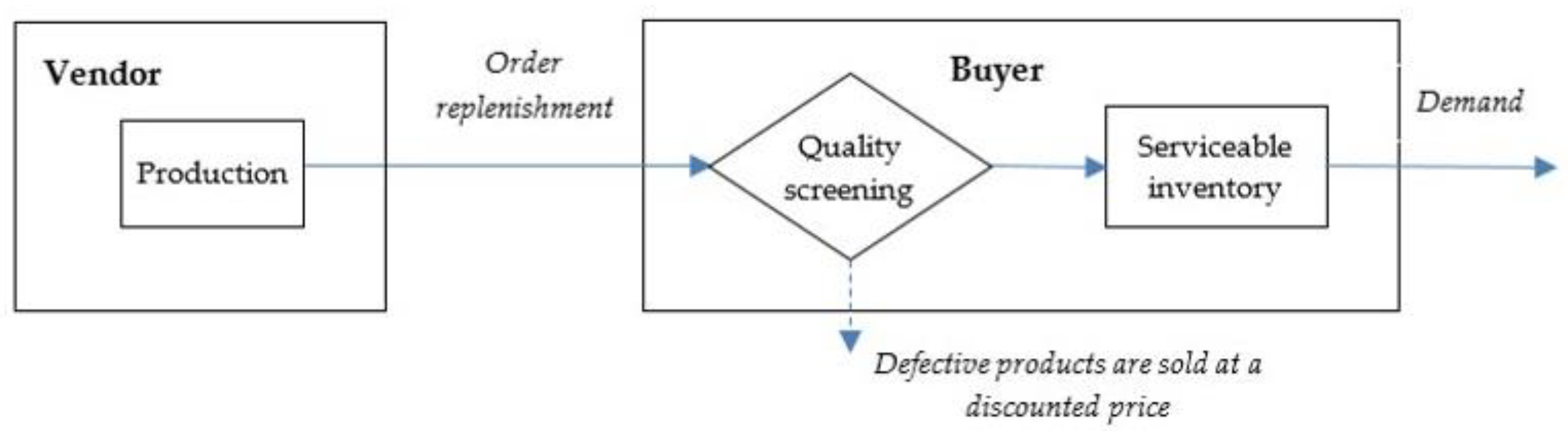
4.1. Model Development with Retailer Inspection
4.1.1. Retailer Cost and Emission
4.1.2. Manufacturer Cost and Emission
4.1.3. The Integrated Manufacturer and Retailer Cost Function
4.1.4. Methodology and Solution Search
- Step 1.
- Substitute the T1 and T functions in Equations (15) and (16) into ETC;
- Step 2.
- Input all the known parameters;
- Step 3.
- Set n = 1;
- Step 4.
- Derive the partial derivative of ETC with respect to T2 and set it to zero. Solve the equation to find the value of T2;
- Step 5.
- Use the known n and T2 to find the value of T1 and T using Equations (15) and (16).
- Step 6.
- Derive the corresponding ETC;
- Step 7.
- If ETC(n) > ETC(n − 1), then n* = n − 1 and go to Step 8; otherwise, set n = n + 1 and go back to Step 4;
- Step 8.
- Use n* and the corresponding T* to find Q* from Equation (4) and calculate R = PT1*.
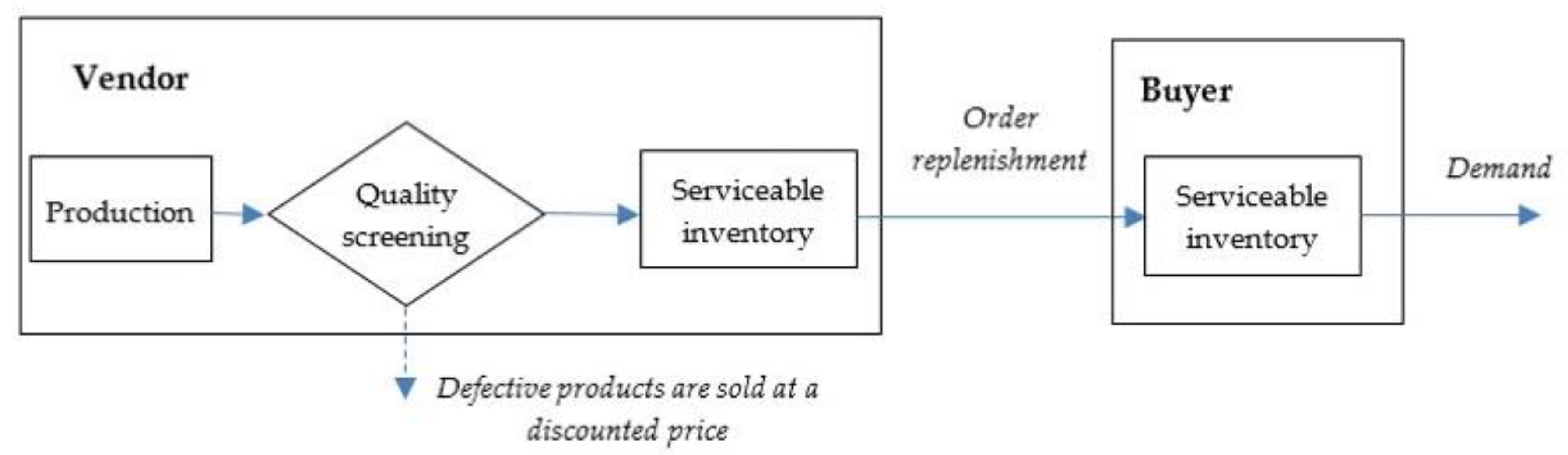
4.2. Model Development with Manufacturer Inspection
4.2.1. Retailer Cost and Emission
4.2.2. Manufacturer Cost and Emission
4.2.3. The Integrated Manufacturer and Retailer Cost Function
4.2.4. Methodology and Solution Search
- Step 1.
- Substitute the T1 and T functions in Equations (36) and (37) into ETC;
- Step 2.
- Input all the known parameters;
- Step 3.
- Set n = 1;
- Step 4.
- Derive the partial derivative of ETC with respect to T2 and set it to zero. Solve the equation to find the value of T2;
- Step 5.
- Use the known n and T2 to find the value of T1 and T using Equations (36) and (37).
- Step 6.
- Derive the corresponding ETC;
- Step 7.
- If ETC(n) > ETC(n-1) then n* = n − 1 and go to step 8, otherwise set n = n + 1 and back to Step 4;
- Step 8.
- Use n* and the corresponding T* to find Q* from Equation (24) and calculate R = PT1*.
5. Numerical Example and Management Insights
5.1. Numerical Example 1
5.2. Numerical Example 2
6. Conclusions and Future Research
Author Contributions
Funding
Acknowledgments
Conflicts of Interest
References
- Glock, C.H. The joint economic lot size problem: A review. Int. J. Prod. Econ. 2012, 135, 671–686. [Google Scholar] [CrossRef]
- Luo, Z.; Gunasekaran, A.; Dubey, R.; Childe, S.J.; Papadopoulos, T. Antecedents of low carbon emissions supply chains. Int. J. Clim. Chang. Strateg. Manag. 2017, 9, 707–727. [Google Scholar] [CrossRef]
- Das, C.; Jharkharia, S. Low carbon supply chain: A state-of-the-art literature review. J. Manuf. Technol. Manag. 2018, 29, 398–428. [Google Scholar] [CrossRef]
- Kazemi, N.; Abdul-Rashid, S.H.; Ghazilla, R.A.R.; Shekarian, E.; Zanoni, S. Economic order quantity models for items with imperfect quality and emission considerations. Int. J. Syst. Sci. Oper. Logist. 2018, 5, 99–115. [Google Scholar] [CrossRef]
- Sarkar, B.; Ahmed, W.; Choi, S.B.; Tayyab, M. Sustainable inventory management for environmental impact through partial backordering and multi-trade-credit period. Sustainability 2018, 10, 4761. [Google Scholar] [CrossRef]
- Taleizadeh, A.A.; Soleymanfar, V.R.; Govindan, K. Sustainable economic production quantity models for inventory system with shortage. J. Clean. Prod. 2018, 174, 1011–1020. [Google Scholar] [CrossRef]
- Sarkar, B.; Ganguly, B.; Sarkar, M.; Pareek, S. Effect of variable transportation and carbon emission in a three-echelon supply chain model. Transp. Res. Part E Logist. Transp. Rev. 2016, 91, 112–128. [Google Scholar] [CrossRef]
- Sarkar, B.; Ahmed, W.; Kim, N. Joint effects of variable carbon emission cost and multi-delay-in-payments under single-setup-multiple-delivery policy in a global sustainable supply chain. J. Clean. Prod. 2018, 185, 421–445. [Google Scholar] [CrossRef]
- Daryanto, Y.; Wee, H.M. Single vendor-buyer integrated inventory model for deteriorating items considering carbon emission. In Proceedings of the 8th International Conference on Industrial Engineering and Operations Management (IEOM), Bandung, Indonesia, 6–8 March 2018; pp. 544–555. [Google Scholar]
- Wahab, M.I.M.; Mamun, S.M.H.; Ongkunarak, P. EOQ models for a coordinated two-level international supply chain considering imperfect items and environmental impact. Int. J. Prod. Econ. 2011, 134, 151–158. [Google Scholar] [CrossRef]
- Jauhari, W.A.; Pamuji, A.S.; Rosyidi, C.N. Cooperative inventory model for vendor-buyer system with unequal-sized shipment, defective items and carbon emission cost. Int. J. Logist. Syst. Manag. 2014, 19, 163–186. [Google Scholar] [CrossRef]
- Sarkar, B.; Saren, S.; Sarkar, M.; Seo, Y.W. A Stackelberg game approach in an integrated inventory model with carbon-emission and setup cost reduction. Sustainability 2016, 8, 1244. [Google Scholar] [CrossRef]
- Jauhari, W.A. A collaborative inventory model for vendor-buyer system with stochastic demand, defective items and carbon emission cost. Int. J. Logist. Syst. Manag. 2018, 29, 241–269. [Google Scholar] [CrossRef]
- Gautam, P.; Khanna, A. An imperfect production inventory model with setup cost reduction and carbon emission for an integrated supply chain. Uncertain Supply Chain Manag. 2018, 6, 271–286. [Google Scholar] [CrossRef]
- Tiwari, S.; Daryanto, Y.; Wee, H.M. Sustainable inventory management with deteriorating and imperfect quality items considering carbon emissions. J. Clean. Prod. 2018, 192, 281–292. [Google Scholar] [CrossRef]
- Rosenblatt, M.J.; Lee, H.L. Economic production cycles with imperfect production processes. IIE Trans. 1986, 18, 48–55. [Google Scholar] [CrossRef]
- Porteus, E.L. Optimal lot sizing, process quality improvement and setup cost reduction. Oper. Res. 1986, 34, 137–144. [Google Scholar] [CrossRef]
- Salameh, M.K.; Jaber, M.Y. Economic production quantity model for items with imperfect quality. Int. J. Prod. Econ. 2000, 64, 59–64. [Google Scholar] [CrossRef]
- Huang, C.K. An integrated vendor-buyer cooperative inventory model for items with imperfect quality. Prod. Plan. Control 2002, 13, 355–361. [Google Scholar] [CrossRef]
- Goyal, S.K.; Huang, C.K.; Chen, K.C. A simple integrated production policy of an imperfect item for vendor and buyer. Prod. Plan. Control 2003, 14, 596–602. [Google Scholar] [CrossRef]
- Wee, H.M.; Yu, J.C.P.; Wang, K.J. An integrated production-inventory model for deteriorating items with imperfect quality and shortage backordering considerations. In Proceedings of the International Conference on Computational Science and Its Applications (ICCSA), Glasgow, UK, 8–11 May 2006; Springer: Berlin/Heidelberg, Germany, 2006; pp. 885–897. [Google Scholar]
- Lee, S.; Kim, D. An optimal policy for a single vendor single-buyer integrated production-distribution model with both deteriorating and defective items. Int. J. Prod. Econ. 2014, 147, 161–170. [Google Scholar] [CrossRef]
- Bazan, E.; Jaber, M.Y.; Zanoni, S.; Zavanella, L.E. Vendor managed inventory (VMI) with consignment stock (CS) agreement for a two-level supply chain with an imperfect production process with/without restoration interruptions. Int. J. Prod. Econ. 2014, 157, 289–301. [Google Scholar] [CrossRef]
- Sarkar, B.; Shaw, B.K.; Kim, T.; Sarkar, M.; Shin, D. An integrated inventory model with variable transportation cost, two-stage inspection, and defective items. J. Ind. Manag. Optim. 2017, 13, 1975–1990. [Google Scholar] [CrossRef]
- Yu, H.F.; Hsu, W.K. An integrated inventory model with immediate return for defective items under unequal-sized shipments. J. Ind. Prod. Eng. 2017, 34, 70–77. [Google Scholar] [CrossRef]
- Benjaafar, S.; Li, Y.; Daskin, M. Carbon footprint and the management of supply chains: Insights from simple models. IEEE Trans. Autom. Sci. Eng. 2013, 10, 99–116. [Google Scholar] [CrossRef]
- Fahimnia, B.; Sarkis, J.; Dehghanian, F.; Banihashemi, N.; Rahman, S. The impact of carbon pricing on a closed-loop supply chain: An Australian case study. J. Clean. Prod. 2013, 59, 210–225. [Google Scholar] [CrossRef]
- Bozorgi, A.; Pazour, J.; Nazzal, D. A new inventory model for cold items that considers costs and emissions. Int. J. Prod. Econ. 2014, 155, 114–125. [Google Scholar] [CrossRef]
- Bozorgi, A. Multi-product inventory model for cold items with cost and emission consideration. Int. J. Prod. Econ. 2016, 176, 123–142. [Google Scholar] [CrossRef]
- Hariga, M.; As’ad, R.; Shamayleh, A. Integrated economic and environmental models for a multi stage cold supply chain under carbon tax regulation. J. Clean. Prod. 2017, 166, 1357–1371. [Google Scholar] [CrossRef]
- Ghosh, A.; Jha, J.K.; Sarmah, S.P. Optimizing a two-echelon serial supply chain with different carbon policies. Int. J. Sustain. Eng. 2016, 9, 363–377. [Google Scholar] [CrossRef]
- Toptal, A.; Çetinkaya, B. How supply chain coordination affects the environment: A carbon footprint perspective. Ann. Oper. Res. 2017, 250, 487–519. [Google Scholar] [CrossRef]
- Bouchery, Y.; Ghaffari, A.; Jemai, Z.; Tan, T. Impact of coordination on cost and carbon emissions for a two-echelon serial economic order quantity problem. Eur. J. Oper. Res. 2017, 260, 520–533. [Google Scholar] [CrossRef]
- Dwicahyani, A.R.; Jauhari, W.A.; Rosyidi, C.N.; Laksono, P.W. Inventory decisions in a two-echelon system with remanufacturing, carbon emission, and energy effects. Cogent Eng. 2017, 4, 1–17. [Google Scholar] [CrossRef]
- Li, J.; Su, Q.; Ma, L. Production and transportation outsourcing decisions in the supply chain under single and multiple carbon policies. J. Clean. Prod. 2017, 141, 1109–1122. [Google Scholar] [CrossRef]
- Wangsa, I.D. Greenhouse gas penalty and incentive policies for a joint economic lot size model with industrial and transport emissions. Int. J. Ind. Eng. Comput. 2017, 8, 453–480. [Google Scholar]
- Anvar, S.H.; Sadegheih, A.; Zad, M.A.V. Carbon emission management for greening supply chains at the operational level. Environ. Eng. Manag. J. 2018, 17, 1337–1347. [Google Scholar]
- Hariga, M.; Babekian, S.; Bahroun, Z. Operational and environmental decisions for a two-stage supply chain under vendor managed consignment inventory partnership. Int. J. Prod. Res. 2018. [Google Scholar] [CrossRef]
- Ji, S.; Zhao, D.; Peng, X. Joint decisions on emission reduction and inventory replenishment with overconfidence and low-carbon preference. Sustainability 2018, 10, 1119. [Google Scholar]
- Wang, S.; Ye, B. A comparison between just-in-time and economic order quantity models with carbon emissions. J. Clean. Prod. 2018, 187, 662–671. [Google Scholar] [CrossRef]
- Ghosh, A.; Sarmah, S.P.; Jha, J.K. Collaborative model for a two-echelon supply chain with uncertain demand under carbon tax policy. Sādhanā 2018, 43, 144. [Google Scholar] [CrossRef]
- Ma, X.; Ho, W.; Ji, P.; Talluri, S. Coordinated pricing analysis with the carbon tax scheme in a supply chain. Decis. Sci. 2018, 49, 863–900. [Google Scholar] [CrossRef]
- Darom, N.A.; Hishamuddin, H.; Ramli, R.; Nopiah, Z.M. An inventory model of supply chain disruption recovery with safety stock and carbon emission consideration. J. Clean. Prod. 2018, 197, 1011–1021. [Google Scholar] [CrossRef]
- Huang, H.; He, Y.; Li, D. Pricing and inventory decisions in the food supply chain with production disruption and controllable deterioration. J. Clean. Prod. 2018, 180, 280–296. [Google Scholar] [CrossRef]
- Daryanto, Y.; Wee, H.M.; Astanti, R.D. Three-echelon supply chain model considering carbon emission and item deterioration. Transp. Res. Part E Logist. Transp. Rev. 2019, 122, 368–383. [Google Scholar] [CrossRef]
- Kundu, S.; Chakrabarti, T. A fuzzy rough integrated multi-stage supply chain inventory model with carbon emissions under inflation and time-value of money. Int. J. Math. Oper. Res. 2019, 14, 123–145. [Google Scholar] [CrossRef]
- Shalke, P.N.; Paydar, M.M.; Hajiaghaei-Keshteli, M. Sustainable supplier selection and order allocation through quantity discounts. Int. J. Manag. Sci. Eng. Manag. 2018, 13, 20–32. [Google Scholar]
- Moheb-Alizadeh, H.; Handfield, R. An integrated chance-constrained stochastic model for efficient and sustainable supplier selection and order allocation. Int. J. Prod. Res. 2018, 56, 6890–6916. [Google Scholar] [CrossRef]
- Moheb-Alizadeh, H.; Handfield, R. Sustainable supplier selection and order allocation: A novel multi-objective programming model with a hybrid solution approach. Comput. Ind. Eng. 2019, 129, 192–209. [Google Scholar] [CrossRef]
- Cao, W.; Hu, Y.; Li, C.; Wang, X. Single setup multiple delivery model of JIT system. Int. J. Adv. Manuf. Technol. 2007, 33, 1222–1228. [Google Scholar] [CrossRef]
- Volvo Truck Corporation. Emissions from Volvo’s Truck. Issue 3. 09 March 2018. Available online: http://www.volvotrucks.com/content/dam/volvo/volvo-trucks/markets/global/pdf/our-trucks/Emis_eng_10110_14001.pdf (accessed on 25 September 2018).
- Yang, P.C.; Wee, H.M. Economic ordering policy of deteriorated item for vendor and buyer: An integrated approach. Prod. Plan. Control 2000, 11, 474–480. [Google Scholar] [CrossRef]
- Jaggi, C.K.; Goel, S.K.; Mittal, M. Economic order quantity model for deteriorating items with imperfect quality and permissible delay in payment. Int. J. Ind. Eng. Comput. 2011, 2, 237–248. [Google Scholar] [CrossRef]
- Swenseth, S.R.; Godfrey, M.R. Incorporating transportation costs into inventory replenishment decisions. Int. J. Prod. Econo. 2002, 77, 113–130. [Google Scholar] [CrossRef]
- Nie, L.; Xu, X.; Zhan, D. Incorporating transportation costs into JIT lot splitting decisions for coordinated supply chains. J. Adv. Manuf. Syst. 2006, 5, 111–121. [Google Scholar] [CrossRef]
- Rahman, M.N.A.; Leuveano, R.A.C.; bin Jafar, F.A.; Saleh, C.; Deros, B.M.; Mahmood, W.M.F.W.; Mahmood, W.H.W. Incorporating logistic costs into a single vendor-buyer JELS model. Appl. Math. Model. 2016, 40, 10809–10819. [Google Scholar] [CrossRef]
- Wangsa, I.D.; Wee, H.M. An integrated vendor-buyer inventory model with transportation cost and stochastic demand. Int. J. Syst. Sci. Oper. Logist. 2018, 5, 295–309. [Google Scholar]
- Hsu, L.F. Erratum to: An optimal policy for a single-vendor single-buyer integrated production-distribution model with both deteriorating and defective items. [Int. J. Prod. Econ. 147 (2014) 161–170]. Int. J. Prod. Econ. 2016, 178, 187–188. [Google Scholar] [CrossRef]
- Misra, R.B. Optimum production lot size model for a system with deteriorating inventory. Int. J. Prod. Res. 1975, 13, 495–505. [Google Scholar] [CrossRef]
- The United States Environmental Protection Agency (US. EPA). Emission Facts: Average Carbon Dioxide Emissions Resulting from Gasoline and Diesel Fuel. February 2005. Available online: https://nepis.epa.gov/ (accessed on 25 September 2018).
- McCarthy, J.E. EPA Standards for Greenhouse Gas Emissions from Power Plants: Many Questions, Some Answers. CRS Report for Congress, 7–5700. 2013. Available online: http://nationalaglawcenter.org/wp-content/uploads/assets/crs/R43127.pdf (accessed on 25 September 2018).
- Goyal, S.K. An integrated inventory model for a single supplier-single customer problem. Int. J. Prod. Res. 1977, 15, 107–111. [Google Scholar] [CrossRef]


| Authors | Imperfect Quality | Deteriorating Item | Variable Transportation Cost | Carbon Emission | |
|---|---|---|---|---|---|
| Vendor’s Inspection | Buyer’s Inspection | ||||
| Huang (2002) | √ | ||||
| Goyal et al. (2003) | √ | ||||
| Wee et al. (2006) | √ | √ | |||
| Wahab et al. (2011) | √ | √ | |||
| Benjaafar et al. (2013) | √ | ||||
| Lee and Kim (2014) | √ | √ | |||
| Bazan et al. (2014) | √ | ||||
| Bozorgi et al. (2014) | √ | ||||
| Jauhari et al. (2014) | √ | √ | |||
| Bozorgi (2016) | √ | ||||
| Ghosh et al. (2016) | √ | ||||
| Sarkar et al. (2016b) | √ | √ | √ | ||
| Yu and Hsu (2017) | √ | ||||
| Sarkar et al. (2017) | √ | √ | |||
| Toptal and Çetinkaya (2017) | √ | ||||
| Bouchery et al. (2017) | √ | ||||
| Dwicahyani et al. (2017) | √ | ||||
| Wangsa (2017) | √ | ||||
| Li et al. (2017) | √ | ||||
| Anvar et al. (2018) | √ | ||||
| Hariga et al. (2018) | √ | ||||
| Ji et al. (2018) | √ | ||||
| Wang and Ye (2018) | √ | ||||
| Gosh et al. (2018) | √ | ||||
| Ma et al. (2018) | √ | ||||
| Darom et al. (2018) | √ | ||||
| Jauhari (2018) | √ | √ | |||
| Gautam and Khanna (2018) | √ | √ | |||
| Wangsa and Wee (2018) | √ | ||||
| Tiwari et al. (2018) | √ | √ | √ | ||
| Kundu and Chakrabarti (2019) | √ | ||||
| This paper | √ | √ | √ | √ | √ |
| Symbol | Definition |
|---|---|
| D | demand rate (unit/year); |
| P | production rate (unit/year); |
| R | production quantity; R = PT1; |
| 𝜃 | deterioration rate; (0 ≤ 𝜃 < 1); |
| u | the probability of defective products per delivery lot size; |
| x | quality screening rate (unit/year); |
| ic | fixed quality inspection cost ($/cycle); |
| uc | unit inspection cost ($/unit); |
| c | retailer’s ordering cost ($/order); |
| hd | retailer’s holding cost ($/unit/year); |
| dd | retailer’s deteriorating cost ($/unit); |
| s | manufacturer’s setup cost ($/order); |
| hp | manufacturer’s holding cost ($/unit/year); |
| dp | manufacturer’s deteriorating cost ($/unit); |
| tf | manufacturer’s fixed transportation cost per delivery ($/delivery); |
| tv | fuel price for manufacturer’s variable transportation cost ($/liter); |
| d | distance traveled from vendor to buyer (km); |
| w | product weight (ton/unit); |
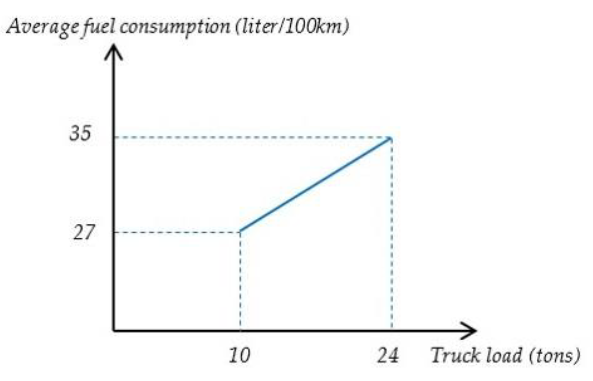
| c1 | average vehicle fuel consumption when empty (liter/km); |
| c2 | average additional fuel consumption per ton of load (liter/km/ton); |
| Tx | carbon emission tax ($/tonCO2); |
| Fe | average emissions from fuel combustion (tonCO2/liter); |
| Ee | average emissions from electricity generation (tonCO2/kWh); |
| e1 | transportation emission cost ($/km); e1 = c1FeTx; |
| e2 | average additional transportation emission cost per unit product ($/unit/km); e2 = c2wFeTx; |
| ec | average warehouse energy consumption per unit product (kWh/unit/year); |
| we | warehouse emissions cost per unit product ($/unit/year); we = ecEeTx; |
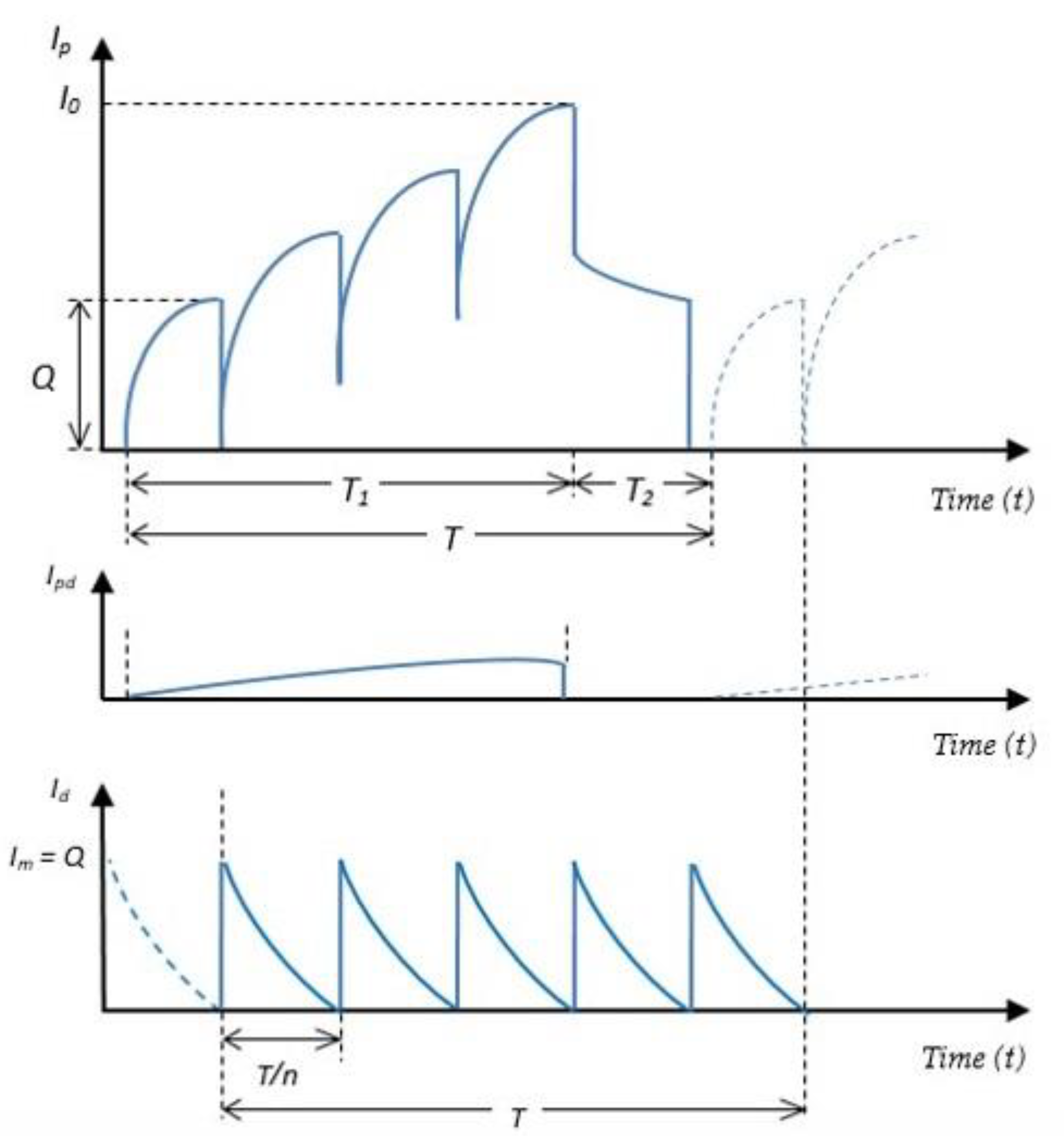
| T | cycle length; |
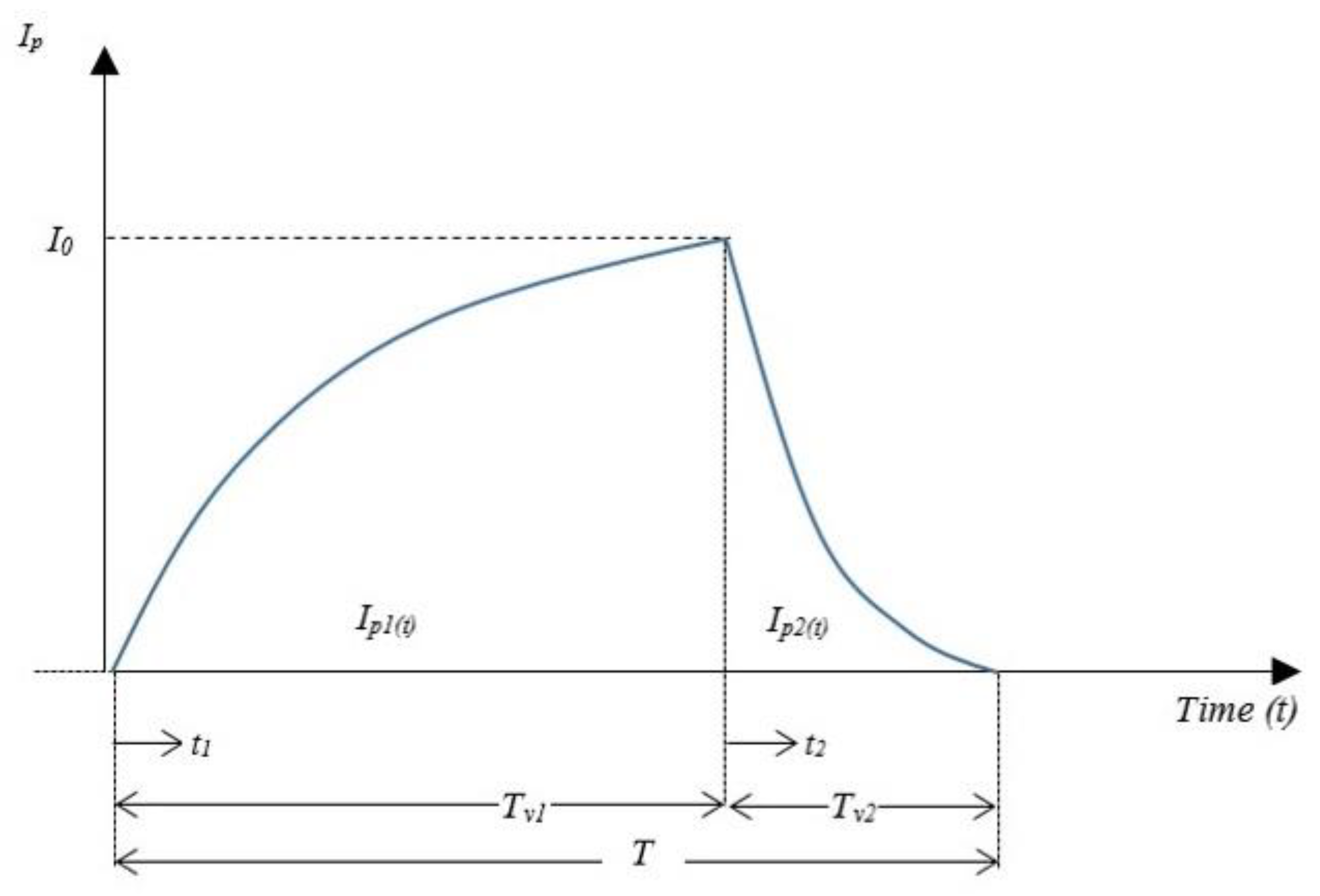
| T1 | production period for the manufacturer in each cycle; |
| T2 | nonproduction period for the manufacturer in each cycle; |
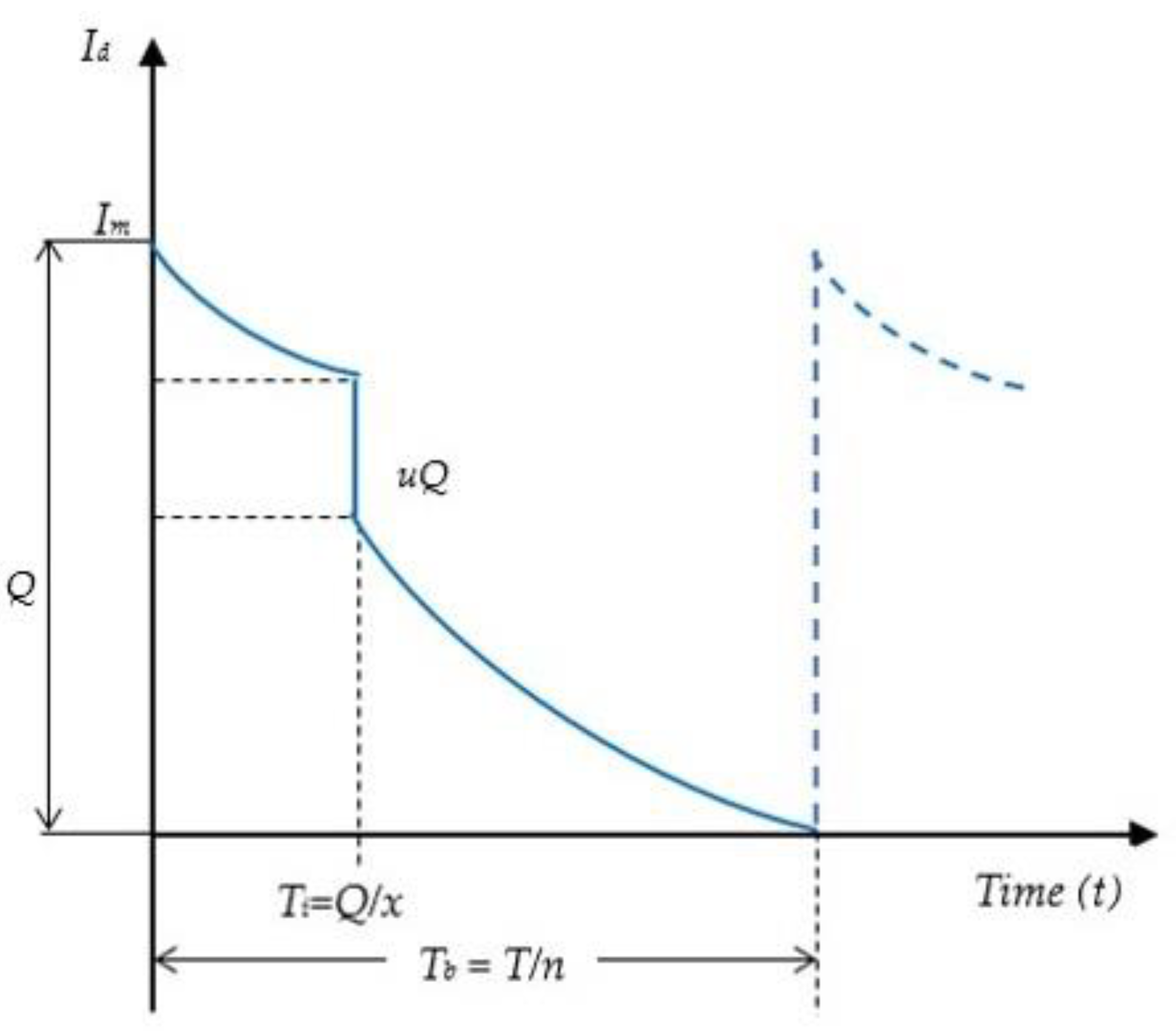
| Ti | inspection time per delivery for the retailer; |
| Tb | inventory cycle length per delivery for the retailer; Tb = T/n; |
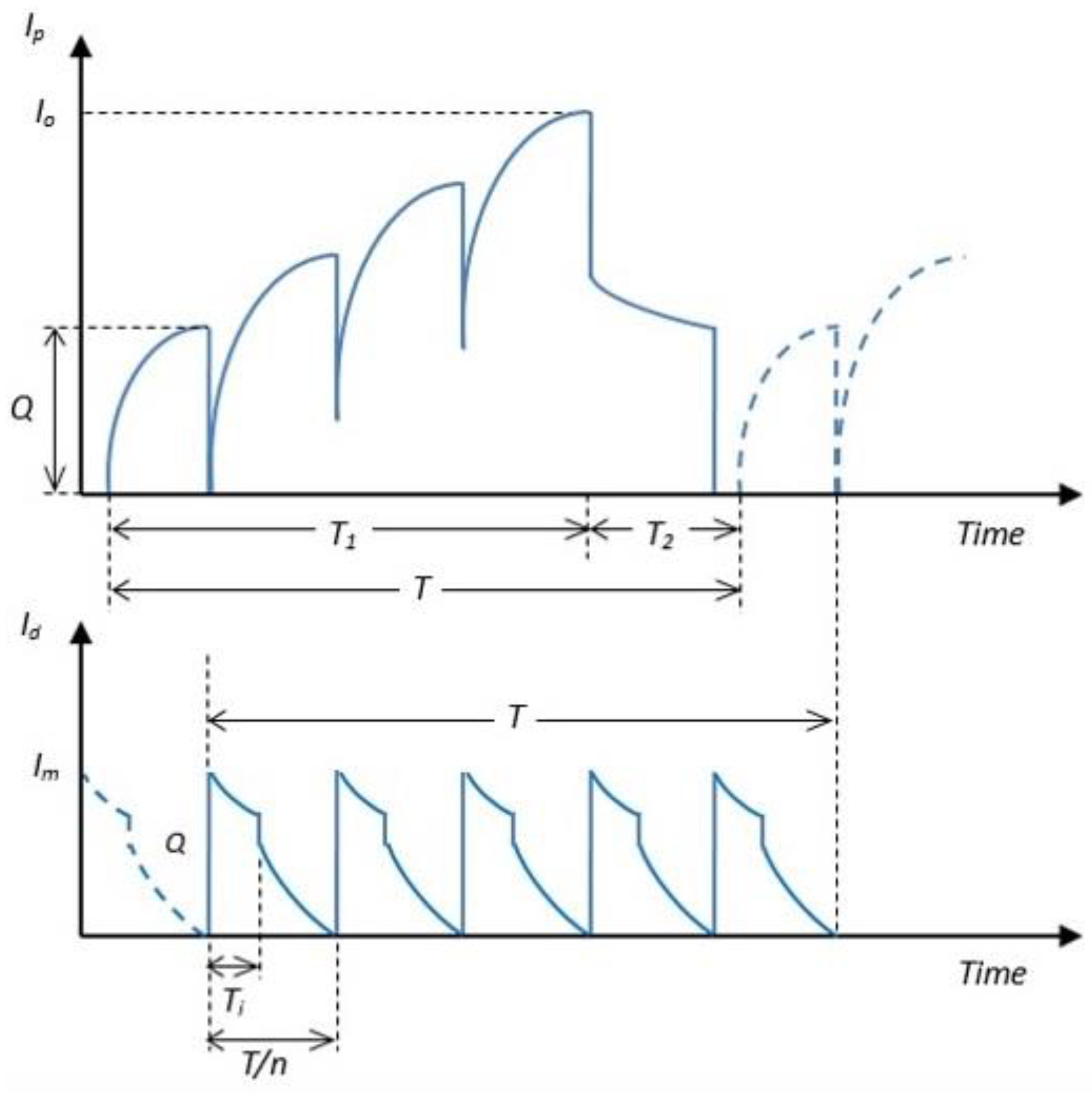
| Ip(t) | manufacturer’s inventory level at time t; |
| Ipd(t) | manufacturer’s inventory for defective products at time t; |
| Id(t) | retailer’s inventory level at time t; |
| ETCd | retailer’s expected total cost per year ($/year); |
| ETCp | manufacturer’s expected total cost per year ($/year); |
| ETC | joint expected total cost per year ($/year); |
| ETEd | retailer’s expected total carbon emissions per year (tonCO2/year); |
| ETEp | manufacturer’s expected total carbon emissions per year (tonCO2/year); |
| ETE | joint expected total carbon emissions per year (tonCO2/year); |
| Decision variables | |
| Q | delivery lot size (unit); |
| n | number of deliveries per order (positive integer). |
| * | indicates optimal solution |
| n | T2(10−5) | T1 (10−5) | T (10−5) | ETCd | ETCp | ETC | ETE |
|---|---|---|---|---|---|---|---|
| 1 | 4960 | 1703 | 6663 | 2,348,991 | 1,017,400 | 3,366,391 | 18.460 |
| 2 | 5641 | 1937 | 7578 | 1,463,323 | 1,568,493 | 3,031,816 | 21.333 |
| 3 | 5961 | 2048 | 8009 | 1,122,012 | 1,799,193 | 2,921,205 | 23.501 |
| 4 | 6161 | 2117 | 8278 | 941,509 | 1,930,509 | 2,872,018 | 25.422 |
| 5 | 6306 | 2167 | 8473 | 830,673 | 2,017,748 | 2,848,421 | 27.216 |
| 6 | 6422 | 2206 | 8628 | 756,370 | 2,081,526 | 2,837,896 | 28.935 |
| 7 * | 6518 | 2240 | 8758 | 703,611 | 2,131,311 | 2,834,922 | 30.598 |
| 8 | 6603 | 2269 | 8872 | 664,620 | 2,172,067 | 2,836,687 | 32.218 |
| 9 | 6680 | 2295 | 8976 | 634,952 | 2,206,651 | 2,841,603 | 33.805 |
| 10 | 6751 | 2320 | 9071 | 611,889 | 2,236,823 | 2,848,712 | 35.360 |
| n | T2(10−5) | T1(10−5) | T (10−5) | ETCd | ETCp | ETC | ETE |
|---|---|---|---|---|---|---|---|
| 1 | 4977 | 1709 | 6686 | 2,041,005 | 1,312,795 | 3,353,800 | 18.22 |
| 2 | 5653 | 1941 | 7595 | 1,167,506 | 1,844,193 | 3,011,699 | 21.07 |
| 3 | 5963 | 2048 | 8011 | 827,178 | 2,067,759 | 2,894,937 | 23.21 |
| 4 | 6151 | 2113 | 8264 | 644,684 | 2,195,273 | 2,839,957 | 25.12 |
| 5 | 6282 | 2158 | 8441 | 530,652 | 2,280,088 | 2,810,741 | 26.91 |
| 6 | 6384 | 2193 | 8577 | 425,568 | 2,342,142 | 2,794,711 | 28.63 |
| 7 | 6467 | 2222 | 8689 | 395,714 | 2,390,607 | 2,786,322 | 30.29 |
| 8 | 6538 | 2246 | 8784 | 352,240 | 2,430,297 | 2,782,747 | 31.92 |
| 9 * | 6601 | 2268 | 8869 | 318,411 | 2,463,985 | 2,782,396 | 33.52 |
| 10 | 6658 | 2288 | 8945 | 290,923 | 2,493,378 | 2,784,301 | 35.11 |
| Decision Variables and Cost Items | Model 1 | Model 2 | Saving (%) |
|---|---|---|---|
| Number of deliveries per cycle (n*) | 7 | 9 | |
| Cycle time (T) | 0.08758 | 0.08869 | |
| Delivery lot size (Q); units | 6387.7 | 4929.6 | |
| Ordering cost ($) | 22,835.7 | 22,550.7 | 1.25 |
| Inspection cost ($) | 295,230.7 | 0 | 100 |
| Inventory holding cost ($) | 190,027.5 | 147,863.7 | 22.2 |
| Deteriorating cost ($) | 195,346.3 | 147,863.7 | 24.3 |
| Emission cost ($) | 171.0 | 133.1 | 22.2 |
| Total retailer’s cost per year ($) | 703,611.2 | 318,909.1 | 54.7 |
| Total retailer’s cost per year after compensation ($) | 690,574.4 | 1.85 | |
| Setup cost ($) | 1,141,784.6 | 1,127,534.2 | 1.25 |
| Inspection cost ($) | 0 | 261,366.3 | −100 |
| Transportation cost ($) | 85,289.5 | 107,690.0 | −26.3 |
| Inventory holding cost ($) | 539,976.9 | 567,658.3 | −5.13 |
| Deteriorating cost ($) | 362,122.2 | 397,345.0 | −9.73 |
| Emission cost ($) | 2,138.0 | 2390.9 | −11.8 |
| Total manufacturer’s cost per year ($) | 2,131,311.2 | 2,463,984.8 | −15.6 |
| Total manufacturer’s cost per year after compensation ($) | 2,091,821.6 | 1.85 | |
| Expected total cost ($) | 2,834,922.4 | 2,782,396.0 | 1.85 |
| Expected total emission (tonCO2/year) | 30.598 | 33.523 | −9.56 |
| Decision Variables and Cost Items | Model 1 | Model 2 adj | Saving (%) |
|---|---|---|---|
| Number of deliveries per cycle (n*) | 7 | 7 | |
| Cycle time (T) | 0.08758 | 0.08704 | |
| Delivery lot size (Q); units | 6,387.7 | 6221.2 | |
| Ordering cost ($) | 22,835.7 | 22,977.4 | −0.62 |
| Inspection cost ($) | 295,230.7 | 0 | 100 |
| Inventory holding cost ($) | 190,027.5 | 186,596.1 | 1.80 |
| Deteriorating cost ($) | 195,346.3 | 186,596.1 | 4.48 |
| Emission cost ($) | 171.0 | 167.9 | 1.81 |
| Total retailer’s cost per year ($) | 703,611.2 | 396,337.5 | 43.7 |
| Total retailer’s cost per year after compensation ($) | 690,428.8 | 1.87 | |
| Setup cost ($) | 1,141,784.6 | 1,148,869.4 | −0.62 |
| Inspection cost ($) | 0 | 261,461.4 | −100 |
| Transportation cost ($) | 85,289.5 | 85,764.5 | −0.55 |
| Inventory holding cost ($) | 539,976.9 | 529,446.7 | 1.95 |
| Deteriorating cost ($) | 362,122.2 | 357,812.1 | 1.20 |
| Emission cost ($) | 2,138.0 | 2117.7 | 0.95 |
| Total manufacturer’s cost per year ($) | 2,131,311.2 | 2,385,471.8 | −11.9 |
| Total manufacturer’s cost per year after compensation ($) | 2,091,380.5 | 1.87 | |
| Expected total cost ($) | 2,834,922.4 | 2,781,809.3 | 1.87 |
| Expected total emission (tonCO2/year) | 30.598 | 30.292 | 1.00 |
| Parameter | Value Change | Model 1 | Model 2 | ||||||||
|---|---|---|---|---|---|---|---|---|---|---|---|
| n * | T | Q a | ETC | %CTC | n * | T | Q b | ETC | %CTC | ||
| P = 2,000,000 | +50% | 7 | 0.0816 | 5949.3 | 3,024,249 | 6.68 | 8 | 0.0819 | 5120.3 | 2,966,117.1 | 6.60 |
| +25% | 7 | 0.0839 | 6117.1 | 2,948,615 | 4.01 | 8 | 0.0842 | 5263.2 | 2,892,821.2 | 3.97 | |
| 0 | 7 | 0.0876 | 6387.7 | 2,834,922 | 0 | 9 | 0.0887 | 4929.6 | 2,782,396.0 | 0 | |
| −25% | 8 | 0.0959 | 6120.6 | 2,643,862 | −6.74 | 9 | 0.0957 | 5322.0 | 2,596,679.1 | −6.67 | |
| −50% | 8 | 0.1147 | 7321.0 | 2,253,495 | −20.5 | 11 | 0.1153 | 5296.5 | 2,217,427.4 | −20.3 | |
| D = 500,000 | +50% | 8 | 0.0816 | 7811.6 | 3,190,858 | 12.5 | 10 | 0.0822 | 6168.2 | 3,136,392.1 | 12.7 |
| +25% | 8 | 0.0841 | 6705.8 | 3,044,190 | 7.38 | 9 | 0.0840 | 5833.6 | 2,989,178.5 | 7.43 | |
| 0 | 7 | 0.0876 | 6387.7 | 2,834,922 | 0 | 9 | 0.0887 | 4929.6 | 2,782,396.0 | 0 | |
| −25% | 7 | 0.0958 | 5242.7 | 2,548,150 | −10.1 | 8 | 0.0962 | 4510.9 | 2,499,238.8 | −10.2 | |
| −50% | 6 | 0.1100 | 4683.3 | 2,151,051 | −24.1 | 8 | 0.1120 | 3501.7 | 2,108,977.7 | −24.2 | |
| c = 2000 | +50% | 7 | 0.0880 | 6415.9 | 2,846,315 | 0.40 | 9 | 0.0891 | 4951.6 | 2,793,646.2 | 0.40 |
| +25% | 7 | 0.0878 | 6401.8 | 2,840,625 | 0.20 | 9 | 0.0889 | 4940.6 | 2,788,027.5 | 0.20 | |
| 0 | 7 | 0.0876 | 6387.7 | 2,834,922 | 0 | 9 | 0.0887 | 4929.6 | 2,782,396.0 | 0 | |
| −25% | 7 | 0.0874 | 6373.5 | 2,829,207 | −0.20 | 9 | 0.0885 | 4918.6 | 2,776,752.0 | −0.20 | |
| −50% | 7 | 0.0872 | 6359.3 | 2,823,479 | −0.40 | 9 | 0.0883 | 4907.5 | 2,771,095.4 | −0.41 | |
| s = 100,000 | +50% | 9 | 0.1074 | 6090.8 | 3,348,784 | 18,1 | 11 | 0.1081 | 4917.3 | 3,292,159.7 | 18.3 |
| +25% | 8 | 0.0979 | 6250.1 | 3,104,546 | 9.51 | 10 | 0.0988 | 4945.1 | 3,049,823.5 | 9.61 | |
| 0 | 7 | 0.0876 | 6387.7 | 2,834,922 | 0 | 9 | 0.0887 | 4929.6 | 2,782,396.0 | 0 | |
| −25% | 6 | 0.0760 | 6464.7 | 2,529,737 | −10.8 | 8 | 0.0773 | 4834.4 | 2,480,006.3 | −10.9 | |
| −50% | 5 | 0.0625 | 6383.9 | 2,169,316 | −23.5 | 6 | 0.0631 | 5257.7 | 2,122,805.7 | −23.7 | |
| ic = 500 | +50% | 7 | 0.0883 | 6437.1 | 2,854,827 | 0.70 | 9 | 0.0888 | 4935.1 | 2,785,213.3 | 0.10 |
| +25% | 7 | 0.0879 | 6412.4 | 2,844,894 | 0.35 | 9 | 0.0887 | 4932.4 | 2,783,805.1 | 0.05 | |
| 0 | 7 | 0.0876 | 6387.7 | 2,834,922 | 0 | 9 | 0.0887 | 4929.6 | 2,782,396.0 | 0 | |
| −25% | 7 | 0.0872 | 6362.9 | 2,824,912 | −0.35 | 9 | 0.0886 | 4926.8 | 2,780,986.3 | −0.05 | |
| −50% | 7 | 0.0869 | 6338.0 | 2,814,883 | −0.71 | 9 | 0.0886 | 4924.1 | 2,779,575.6 | −0.10 | |
| uc = 0.5 | +50% | 7 | 0.0876 | 6387.5 | 2,962,557 | 4.50 | 9 | 0.0887 | 4929.0 | 2,910,260.4 | 4.60 |
| +25% | 7 | 0.0876 | 6387.6 | 2,898,740 | 2.25 | 9 | 0.0887 | 4929.3 | 2,846,328.1 | 2.30 | |
| 0 | 7 | 0.0876 | 6387.7 | 2,834,922 | 0 | 9 | 0.0887 | 4929.6 | 2,782,396.0 | 0 | |
| −25% | 7 | 0.0876 | 6387.8 | 2,771,105 | −2.25 | 9 | 0.0887 | 4929.9 | 2,718,463.9 | −2.30 | |
| –50% | 7 | 0.0876 | 6387.9 | 2,707,289 | −4.50 | 9 | 0.0887 | 4930.2 | 2,654,531.7 | −4.60 | |
| hd = 60 | +50% | 9 | 0.0872 | 4947.9 | 2,916,253 | 2,87 | 11 | 0.0880 | 4003.7 | 2,848,604.1 | 2.38 |
| +25% | 8 | 0.0873 | 5571.5 | 2,878,457 | 1.54 | 10 | 0.0883 | 4014.8 | 2,817,636.9 | 1.27 | |
| 0 | 7 | 0.0876 | 6387.7 | 2,834,922 | 0 | 9 | 0.0887 | 4929.6 | 2,782,396.0 | 0 | |
| −25% | 6 | 0.0882 | 7502.8 | 2,782,702 | −1.84 | 7 | 0.0885 | 6327.8 | 2,739,318.4 | −1.55 | |
| −50% | 5 | 0.0893 | 9119.2 | 2,716,341 | −4.18 | 5 | 0.0889 | 8901.6 | 2,680,745.8 | −3.65 | |
| hp = 40 | +50% | 5 | 0.0779 | 7955.9 | 3,075,129 | 8.47 | 5 | 0.0776 | 7768.5 | 3,033,547.3 | 9.03 |
| +25% | 6 | 0.0823 | 7002.8 | 2,962,650 | 4.51 | 7 | 0.0827 | 5908.5 | 2,915,155.6 | 4.77 | |
| 0 | 7 | 0.0876 | 6387.7 | 2,834,922 | 0 | 9 | 0.0887 | 4929.6 | 2,782,396.0 | 0 | |
| −25% | 8 | 0.0940 | 5999.5 | 2,691,834 | −5.05 | 10 | 0.0951 | 4758.0 | 2,634,200.0 | −5.33 | |
| −50% | 9 | 0.1020 | 5786.3 | 2,531,836 | −10.7 | 13 | 0.1051 | 4044.5 | 2,468,523.7 | −11.3 | |
| dd = 600 | +50% | 9 | 0.0872 | 49441 | 2,918,318 | 2,94 | 11 | 0.0880 | 4003.7 | 2,848,604.1 | 2.38 |
| +25% | 8 | 0.0873 | 5569.0 | 2,879,619 | 1.58 | 10 | 0.0883 | 4416.4 | 2,817,636.9 | 1.27 | |
| 0 | 7 | 0.0876 | 6387.7 | 2,834,922 | 0 | 9 | 0.0887 | 4929.6 | 2,782,396.0 | 0 | |
| −25% | 6 | 0.0882 | 7507.4 | 2,781,144 | −1.90 | 7 | 0.0885 | 6327.8 | 2,739,318.4 | −1.55 | |
| −50% | 3 | 0.0872 | 14852.7 | 2,703,928 | −4.62 | 5 | 0.0889 | 8901.6 | 2,680,745.8 | −3.65 | |
| dp = 400 | +50% | 7 | 0.0820 | 5981.9 | 3,010,061 | 6,18 | 6 | 0.0806 | 6721.3 | 2,957,798.8 | 6.30 |
| +25% | 7 | 0.0847 | 6174.8 | 2,923,924 | 3.14 | 7 | 0.0839 | 5999.6 | 2,875,189.0 | 3.33 | |
| 0 | 7 | 0.0876 | 6387.7 | 2,834,922 | 0 | 9 | 0.0887 | 4929.6 | 2,782,396.0 | 0 | |
| −25% | 8 | 0.0922 | 5884.4 | 2,738,923 | −3.39 | 10 | 0.0933 | 4668.1 | 2,679,457.1 | −3.70 | |
| −50% | 9 | 0.0976 | 5538.2 | 2,632,492 | −7.14 | 12 | 0.0997 | 4155.5 | 2,566,509.0 | −7.76 | |
| 𝜃 = 0.1 | +50% | 7 | 0.0794 | 5794.4 | 3,100,001 | 9.35 | 9 | 0.0804 | 4470.6 | 3,041,924.7 | 9.33 |
| +25% | 7 | 0.0832 | 6069.2 | 2,970,737 | 4.79 | 9 | 0.0843 | 4683.2 | 2,915,364.1 | 4.78 | |
| 0 | 7 | 0.0876 | 6387.7 | 2,834,922 | 0 | 9 | 0.0887 | 4929.6 | 2,782,396.0 | 0 | |
| −25% | 7 | 0.0927 | 6762.9 | 2,691,447 | −5.06 | 9 | 0.0939 | 5219.8 | 2,641,938.0 | −5.05 | |
| −50% | 7 | 0.0989 | 7213.9 | 2,538,850 | −10.4 | 8 | 0.0992 | 5516.8 | 2,492,404.9 | −10.4 | |
| tf = 1000 | +50% | 6 | 0.0874 | 7440.5 | 2,872,436 | 1.32 | 7 | 0.0883 | 6308.3 | 2,826,288.0 | 1.58 |
| +25% | 7 | 0.0883 | 6437.1 | 2,854,827 | 0.70 | 8 | 0.0886 | 5542.6 | 2,805,413.7 | 0.83 | |
| 0 | 7 | 0.0876 | 6387.7 | 2,834,922 | 0 | 9 | 0.0887 | 4929.6 | 2,782,396.0 | 0 | |
| −25% | 8 | 0.0879 | 5612.0 | 2,814,046 | −0.74 | 10 | 0.0885 | 4425.0 | 2,756,197.9 | −0.94 | |
| −50% | 9 | 0.0880 | 4991.1 | 2,790,972 | −1.55 | 12 | 0.0884 | 3685.7 | 2,725,660.0 | −2.04 | |
| tv = 0.75 | +50% | 7 | 0.0876 | 6391.8 | 2,837,605 | 0.09 | 9 | 0.0888 | 4933.7 | 2,785,501.1 | 0.11 |
| +25% | 7 | 0.0876 | 6389.7 | 2,836,264 | 0.05 | 9 | 0.0887 | 4931.6 | 2,783,948.8 | 0.06 | |
| 0 | 7 | 0.0876 | 6387.7 | 2,834,922 | 0 | 9 | 0.0887 | 4929.6 | 2,782,396.0 | 0 | |
| −25% | 7 | 0.0876 | 6385.7 | 2,833,581 | −0.05 | 9 | 0.0886 | 4927.6 | 2,780,842.7 | −0.06 | |
| −50% | 7 | 0.0875 | 6383.6 | 2,832,239 | −0.09 | 9 | 0.0886 | 4925.5 | 2,779,289.1 | −0.11 | |
| d = 100 | +50% | 7 | 0.0877 | 6392.8 | 2,838,309 | 0.12 | 9 | 0.0888 | 4934.7 | 2,786,313.0 | 0.14 |
| +25% | 7 | 0.0876 | 6390.3 | 2,836,616 | 0.06 | 9 | 0.0887 | 4932.2 | 2,784,355.0 | 0.07 | |
| 0 | 7 | 0.0876 | 6387.7 | 2,834,922 | 0 | 9 | 0.0887 | 4929.6 | 2,782,396.0 | 0 | |
| −25% | 7 | 0.0875 | 6385.1 | 2,833,229 | −0.06 | 9 | 0.0886 | 4927.0 | 2,780,436.7 | −0.07 | |
| −50% | 7 | 0.0875 | 6382.6 | 2,831,535 | −0.12 | 9 | 0.0886 | 4924.5 | 2,778,476.4 | −0.14 | |
| E[u] = 0.02 | +50% | 7 | 0.0874 | 6437.8 | 2,843,908 | 0.32 | 9 | 0.0887 | 4931.3 | 2,784,137.7 | 0.063 |
| +25% | 7 | 0.0875 | 6412.6 | 2,839,414 | 0.16 | 9 | 0.0887 | 4930.5 | 2,783,248.6 | 0.031 | |
| 0 | 7 | 0.0876 | 6387.7 | 2,834,922 | 0 | 9 | 0.0887 | 4929.6 | 2,782,396.0 | 0 | |
| −25% | 7 | 0.0877 | 6363.1 | 2,830,435 | −0.16 | 9 | 0.0887 | 4928.7 | 2,781,579.0 | −0.029 | |
| −50% | 7 | 0.0878 | 6338.7 | 2,825,951 | −0.32 | 9 | 0.0887 | 4927.7 | 2,780,796.5 | −0.058 | |
| w = 0.01 | +50% | 7 | 0.0876 | 6387.7 | 2,835,956 | 0.04 | 9 | 0.0887 | 4929.6 | 2,783,408.9 | 0.036 |
| +25% | 7 | 0.0876 | 6387.7 | 2,835.439 | 0.02 | 9 | 0.0887 | 4929.6 | 2,782,902.6 | 0.018 | |
| 0 | 7 | 0.0876 | 6387.7 | 2,834,922 | 0 | 9 | 0.0887 | 4929.6 | 2,782,396.0 | 0 | |
| −25% | 7 | 0.0876 | 6387.7 | 2,834,405 | −0.02 | 9 | 0.0887 | 4929.6 | 2,781,889.5 | −0.018 | |
| −50% | 7 | 0.0876 | 6.387.7 | 2,833,889 | −0.04 | 9 | 0.0887 | 4929.6 | 2,781,383.0 | −0.036 | |
| c1, c2= 0.27, 0.0057 | +50% | 7 | 0.0876 | 6388.7 | 2,835,627 | 0.02 | 9 | 0.0887 | 4930.5 | 2,783,244.8 | 0.031 |
| +25% | 7 | 0.0876 | 6388.2 | 2,835,275 | 0.01 | 9 | 0.0887 | 4930.0 | 2,782,838.6 | 0.016 | |
| 0 | 7 | 0.0876 | 6387.7 | 2,834,922 | 0 | 9 | 0.0887 | 4929.6 | 2,782,396.0 | 0 | |
| −25% | 7 | 0.0876 | 6387.2 | 2,834,570 | −0.01 | 9 | 0.0887 | 4928.9 | 2,782,026.3 | −0.013 | |
| −50% | 7 | 0.0876 | 6386.7 | 2,834,218 | −0.02 | 9 | 0.0887 | 4928.4 | 2,781,620.2 | −0.028 | |
| ec = 1.44 | +50% | 7 | 0.0876 | 6386.6 | 2,835,372 | 0.016 | 9 | 0.0887 | 4928.7 | 2,782,845.7 | 0.016 |
| +25% | 7 | 0.0876 | 6387.1 | 2,835,148 | 0.008 | 9 | 0.0887 | 4929.2 | 2,782,620.8 | 0.008 | |
| 0 | 7 | 0.0876 | 6387.7 | 2,834,922 | 0 | 9 | 0.0887 | 4929.6 | 2,782,396.0 | 0 | |
| −25% | 7 | 0.0876 | 6388.3 | 2,834,698 | −0.008 | 9 | 0.0887 | 4930.0 | 2,782,171.2 | −0.008 | |
| −50% | 7 | 0.0876 | 6388.8 | 2,834,472 | −0.016 | 9 | 0.0887 | 4930.5 | 2,781,946.2 | −0.016 | |
| Tx = 75 | +50% | 7 | 0.0876 | 6387.7 | 2,836,077 | 0.04 | 9 | 0.0887 | 4929.8 | 2,783,658.0 | 0.045 |
| +25% | 7 | 0.0876 | 6387.7 | 2,835,500 | 0.02 | 9 | 0.0887 | 4929.7 | 2,783,027.1 | 0.023 | |
| 0 | 7 | 0.0876 | 6387.7 | 2,834,922 | 0 | 9 | 0.0887 | 4929.6 | 2,782,396.0 | 0 | |
| −25% | 7 | 0.0876 | 6387.7 | 2,834,345 | −0.02 | 9 | 0.0887 | 4929.5 | 2,781,764.9 | −0.023 | |
| −50% | 7 | 0.0876 | 6387.6 | 2,833,768 | −0.04 | 9 | 0.0887 | 4929.4 | 2,781,134.2 | −0.045 | |
© 2019 by the authors. Licensee MDPI, Basel, Switzerland. This article is an open access article distributed under the terms and conditions of the Creative Commons Attribution (CC BY) license (http://creativecommons.org/licenses/by/4.0/).
Share and Cite
Daryanto, Y.; Wee, H.M.; Widyadana, G.A. Low Carbon Supply Chain Coordination for Imperfect Quality Deteriorating Items. Mathematics 2019, 7, 234. https://doi.org/10.3390/math7030234
Daryanto Y, Wee HM, Widyadana GA. Low Carbon Supply Chain Coordination for Imperfect Quality Deteriorating Items. Mathematics. 2019; 7(3):234. https://doi.org/10.3390/math7030234
Chicago/Turabian StyleDaryanto, Yosef, Hui Ming Wee, and Gede Agus Widyadana. 2019. "Low Carbon Supply Chain Coordination for Imperfect Quality Deteriorating Items" Mathematics 7, no. 3: 234. https://doi.org/10.3390/math7030234
APA StyleDaryanto, Y., Wee, H. M., & Widyadana, G. A. (2019). Low Carbon Supply Chain Coordination for Imperfect Quality Deteriorating Items. Mathematics, 7(3), 234. https://doi.org/10.3390/math7030234