1. Introduction
In 1965, Zadeh [
1] initiated fuzzy set theory which provides a useful mathematical tool for modelling and manipulating uncertainty based on the perspective of gradualness. The notion of fuzzy sets is closely associated with soft computing which deals with imprecision, uncertainty, partial truth and approximation to achieve tractability, robustness and low solution cost [
2]. Atanassov [
3,
4] proposed the concept of intuitionistic fuzzy sets in 1983, which is characterized by membership and non-membership functions. Atanassov’s intuitionistic fuzzy sets extend Zadeh’s fuzzy sets in a meaningful way, due to its convenience to capture uncertainty caused by indecisiveness and lack of commitment in human cognition [
5]. Bustince and Burillo [
6] revealed that the concept of vague sets, proposed by Gau and Buehrer [
7], could be identified with intuitionistic fuzzy sets. Wang and He [
8] showed that intuitionistic fuzzy sets can be seen as
L-fuzzy sets. Deschrijver and Kerre further examined the relationships among fuzzy sets,
L-fuzzy sets, intuitionistic fuzzy sets, interval-valued fuzzy sets and interval-valued intuitionistic fuzzy sets in [
9].
In 1999, Molodtsov [
10] proposed soft set theory as another formal method for handling uncertainty. The rationale of soft sets relies on the idea of parameterization, which suggests that complicated things should be perceived from various aspects, and each aspect only provides an approximate description of the whole entity of high complexity [
11]. Maji et al. [
12] defined a number of algebraic operations for soft sets and examined some related properties. Ali et al. [
13,
14] introduced several new operations in soft set theory to further consolidate theoretical aspects of soft sets. It is worth noting that soft sets are closely related to other soft computing models such as rough sets and fuzzy sets [
15,
16]. Maji et al. [
17] introduced fuzzy soft sets, extending both fuzzy sets and soft sets in a natural way. They further combined soft sets with intuitionistic fuzzy sets, and brought forth the notion of intuitionistic fuzzy soft sets in [
18]. In addition, soft sets and their extensions have been successfully applied to algebra [
19,
20,
21,
22], data analysis [
11,
23], decision making [
24,
25,
26,
27,
28,
29,
30], graph theory [
31] and mathematical logic [
32].
The membership degree and non-membership degree of each element in an intuitionistic fuzzy set can be combined together to form an ordered pair, which was called an intuitionistic fuzzy value (IFV) by Xu and Yager in [
33]. This convenient representation has been widely used in the literature. From the theoretical aspect, it provides a solid basis for constructing and investigating various measures [
34,
35], operations [
36], aggregation operators [
37], ranking methods [
38,
39] and generalizations [
40,
41] of intuitionistic fuzzy sets. From the practical aspect, the use of this representation greatly facilitates the development of decision making [
5,
42,
43,
44,
45] and group decision making [
46,
47,
48] in an intuitionistic fuzzy setting. The modelling and managing of uncertainty is of great importance for the acquisition of desirable solutions to decision making problems. IFVs can be used to describe and quantify subjective uncertainty in human cognition from the aspects of affirmation, objection and hesitation [
45]. This makes them elementary components in multiple attribute decision making (MADM) based on intuitionistic fuzzy sets. As a result, it becomes vital to develop efficient methods for the computation, aggregation and comparison of IFVs. Xu and Yager [
33,
37] proposed some fundamental operations for IFVs, which laid a firm foundation for the aggregation of intuitionistic fuzzy information. Based on the algebraic sum and scalar product operations of IFVs, Xu [
37] further developed the intuitionistic fuzzy weighted averaging (IFWA) operator. To compare IFVs, Chen [
42] proposed the score function, which can synthesize both positive and negative evaluations. Later, Hong and Choi [
49] indicated that the score function is unable to distinguish some apparently different IFVs with the same score. To address this issue, they proposed another useful measure called accuracy function in [
49]. Using both the score function and accuracy function, Xu [
33] pioneered a novel approach to the ranking of IFVs. As pointed out by Bustince et al. [
50], the Xu-Yager order is a lexicographic order refining the usual partial order on the lattice of IFVs. Furthermore, Bustince et al. initiated a general notion called admissible orders and proposed a useful method to build admissible orders by virtue of aggregation functions in [
50].
It is worth noting that lexicographic orders like Xu-Yager order play an indispensable role in comparing IFVs since it is impossible to represent such orders using only one real-valued function. In fact, this can trace back to a famous counter-example called the Debreu chain [
51], which revealed that contrary to the inveterate belief widely held by economists, there indeed exist a preference order relation which is not representable by a utility function. Recently, we proposed two lexicographic orders
and
based on the expectation score function in [
40]. We also showed that the order
coincides with the Xu-Yager order. This paper aims to construct some new lexicographic orders by virtue of the membership, non-membership, score, accuracy and expectation score functions. We present some equivalent characterizations and illustrative examples in order to ascertain abundant relationships among various lexicographic orders. Motivated by the fact that the IFWA operator is often used together with the Xu-Yager order for solving intuitionistic fuzzy MADM problems, we endeavor to explore compatible properties of these lexicographic orders with respect to the algebraic sum and scalar product operations of IFVs. In addition, we revisit a benchmark problem, which was originally raised by Herrera and Herrera-Viedma [
52], and further investigated by Wei [
53], so as to give comparative analysis of different lexicographic orders and highlight the practical value of the obtained results for solving intuitionistic fuzzy MADM problems in real-world scenarios.
The rest of this paper is organized as follows.
Section 2 briefly recalls some basic concepts including fuzzy sets, intuitionistic fuzzy sets and intuitionistic fuzzy soft sets.
Section 3 mainly introduces binary relations and order relations. In
Section 4, we define a variety of new lexicographic orders for comparing IFVs. We also give some equivalent characterizations and illustrative examples so as to ascertain the relationships among various lexicographic orders.
Section 5 is devoted to the investigation of compatible properties of lexicographic orders. In
Section 6, we revisit a benchmark problem regarding risk investment to compare different lexicographic orders and emphasize the pragmatic value of the obtained results for solving real-world intuitionistic fuzzy MADM problems. Finally, we summarize this study and point out possible future works in the last section.
2. Preliminaries
In this section, we recall some basic concepts regarding fuzzy sets, intuitionistic fuzzy sets and intuitionistic fuzzy soft sets. These notions will be useful for subsequent discussion.
Let U be a fixed nonempty set, known as the universe of discourse. A fuzzy set in U is defined by its membership function . For each , the membership degree specifies the grade to which the element x belongs to the fuzzy set . By , we mean that for all . Clearly if and . In what follows, the collection of all fuzzy sets in U will be denoted by .
Definition 1. [
4]
An intuitionistic fuzzy set in a universe U is given bywhere the functions and assign membership grade and non-membership grade of the element x to the intuitionistic fuzzy set A, respectively. In addition, it should be satisfied that for all . Notice that is called the degree of hesitancy (or indeterminacy) of x to A. In the following, denotes the collection of all intuitionistic fuzzy sets in U.
Let . Then we have the following notions:
;
;
if and only if and for all .
By
, we mean that
and
. Clearly, every fuzzy set can be viewed as an intuitionistic fuzzy set. It was shown in [
8,
9] that intuitionistic fuzzy sets can be viewed as
L-fuzzy sets with respect to the complete lattice
, where
, and the corresponding lattice order
is defined as
for all
. Each ordered pair
is called an
intuitionistic fuzzy value. According to this point of view, the intuitionistic fuzzy set
can be identified with the
L-fuzzy set
such that
for all
.
Let
denote the power set of
U and let
(called the parameter space and simply denoted by
E) be the set of all parameters associated with objects in
U. There is no further restriction on parameters. The parameter space
E might be an infinite set even if
U is a finite set. To serve pragmatic purpose, attributes, criteria, or characteristics of objects in
U are often chosen as parameters. Following Molodtsov [
10], a soft set over
U is defined as a pair
, where
and
is a set-valued mapping, called the
approximate function of the soft set
S.
By combining soft sets with intuitionistic fuzzy sets, Maji et al. [
18] initiated the following notion.
Definition 2. [
18]
A pair is called an intuitionistic fuzzy soft set over U, where and is a mapping. 3. Binary Relations and Order Relations
In this section, let us recall some basic notions regarding binary relations and order relations.
Definition 3. A binary relation R between two sets A and B is a subset of the direct product . In particular, is called a (homogeneous) binary relation on A.
Let R be a binary relation between A and B. If , we say that a is R-related b (or are R-related), which is denoted by . The domain of R is the set of all such that for some . The range of R is the set of all such that for some .
Definition 4. A binary relation R on a set A is said to be:
reflexive if for all .
irreflexive (or strict) if for all .
symmetric if , then for all .
antisymmetric if and , then for all .
asymmetric if , then for all .
transitive if and , then for all .
complete if , then or for all .
total (or strong complete) if or for all .
Definition 5. A binary relation ⪯ on a set A is called a preorder if it is reflexive and transitive.
Definition 6. An antisymmetric preorder ⪯ on A is called a partial order.
Definition 7. A complete preorder ⪯ on A is called a weak order.
Definition 8. A weak order ⪯ on A is called a linear order (or total order) if it is antisymmetric.
A set A together with a partial order ⪯ on A is called a poset and is denoted by . If ⪯ is a total order, the poset is called a chain.
Definition 9. [
50]
A partial order ⪯ on is said to be admissible if- (1)
⪯ is a linear order on ;
- (2)
For all , implies .
Definition 10. Let and be two posets. The lexicographic order ⪯ on is defined byfor all . In the above definition, means and . It is easy to show that the lexicographic order ≤ is reflexive, antisymmetric and transitive. Thus it is a partial order on the Cartesian product .
Let
denote the set of all closed subintervals of the unit interval. That is,
With respect to the relation
given by
the set
becomes a poset with the minimum
and the maximum
. In order to extend the partial order
to a linear order, Bustince et al. [
50] introduced the following lexicographic orders of intervals.
Definition 11. [
50]
The binary relation on is defined aswhere and are intervals in . Definition 12. [
50]
The binary relation on is defined aswhere and are intervals in . As shown below, Bustince et al. [
50] pointed out that lexicographic orders like
and
are indispensable since it is impossible to represent them using only one real-valued function.
Theorem 1. [
50]
Let ⪯ be an admissible order on . Then it cannot be induced by means of a single continuous function . 4. Lexicographic Orders of IFVs
The following concept was pioneered by Chen and Tan [
42] to solve MADM problems in an intuitionistic fuzzy setting.
Definition 13. [
42]
The score function is a mapping given by for all . The score function aims to calculate the net effect of positive and negative evaluations. Later, Hong and Choi [
49] pointed out that the score function might fail to differentiate some obviously distinct IFVs with the same score. To overcome this difficulty, they developed another function as follows.
Definition 14. [
49]
The accuracy function is a mapping given by for all . Using the score function and the accuracy function, Xu and Yager [
33] developed a method for comparing IFVs in the following way.
Definition 15. [
33]
Let and be two IFVs. Then can be compared as follows:if , A is smaller than B and denoted by ;
if , then we have:
- (1)
if , A is equivalent to B and denoted by ;
- (2)
if , A is smaller than B and denoted by ;
- (3)
if , A is greater than B and denoted by .
It is worth noting that Definition 15 can be simplified as a binary relation
on the lattice of IFVs:
for all
. The relation
is a linear order on
, which will be called the Xu-Yager lexicographic order of IFVs in the following.
Xu [
37] showed that for all
,
Thus the Xu-Yager lexicographic order is an admissible order on .
Definition 16. [
40]
A partial order ⪯ on is said to be bounded if- (1)
for all ;
- (2)
for all .
Definition 17. [
40]
A partial order ⪯ on is said to be normal if- (1)
and implies for all ;
- (2)
and implies for all .
It is easy to see that every admissible order on is bounded and normal.
Definition 18. [
40]
The expectation score function is a mapping such thatfor all . Based on the expectation score function, Feng et al. [
40] proposed the following lexicographic order of IFVs.
Definition 19. [
40]
Let and be IFVs in . The binary relation on is defined as Theorem 2. [
40]
The relation is an admissible order on . By interchanging the membership grade with the expectation score, Feng et al. [
40] introduced another lexicographic order of IFVs as follows.
Definition 20. [
40]
Let and be IFVs in . The binary relation on is defined as Theorem 3. [
40]
Let and be IFVs in . Then The above assertion indicates that
coincides with the Xu-Yager lexicographic order
. Moreover, Feng et al. [
40] established the following equivalent characterizations for the Xu-Yager lexicographic order.
Theorem 4. [
40]
Let and be IFVs in . Then the following are equivalent:- (1)
;
- (2)
;
- (3)
;
- (4)
;
- (5)
.
Definition 21. Let and be IFVs in . The binary relation on is given by Definition 22. Let and be IFVs in . The binary relation on is given by Corollary 1. Let and be IFVs in . Then Proof. This follows directly from Theorem 4. □
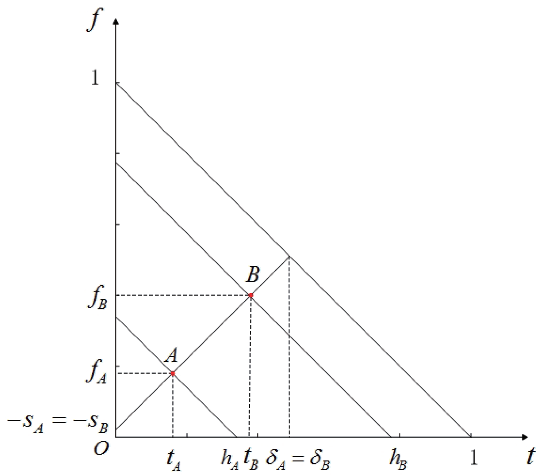
The results established in Theorem 4 and Corollary 1 indicate that the lexicographic orders
,
,
and
, in spite of being defined in terms of different measures, will always produce the same results when we use them to compare or rank IFVs. This equivalence is illustrated by
Figure 1.
Definition 23. Let and be IFVs in . The binary relation on is given by Definition 24. Let and be IFVs in . The binary relation on is given by Corollary 2. Let and be IFVs in . Then Proof. This follows directly from Theorem 4. □
As shown in the example below, and are different lexicographic orders of IFVs.
Example 1. Consider two IFVsandIt is easy to see that , and . Also we have , and . Since and , we deduce that . On the other hand, is not true since and . Similarly, we can show that holds while is not true. This shows that and are different. From Theorem 3, it follows that and are distinct. Using Corollary 1 and Corollary 2, many similar results can easily be deduced, which are no longer stated here.
Motivated by Bustince’s ordering of intervals, we introduce the following order relations for IFVs.
Definition 25. Let and be IFVs in . The binary relation on is given by It is interesting to see that coincides with the order relation .
Theorem 5. Let and be IFVs in . Then if and only if .
Proof. First, suppose that . Then the following two cases should considered.
(1) If , then .
(2) If
and
, we have
Thus
and
. That is,
.
Conversely, assume that . Then we consider the following two cases.
(1) If , then .
(2) If
and
, we have
Thus and . That is, . □
Theorem 6. Let and be IFVs in . Then the following are equivalent:
- (1)
;
- (2)
;
- (3)
;
- (4)
.
Proof. Note first that (1) and (2) are equivalent as shown in the proof of Theorem 5.
Next, we can also show that (1) and (3) are equivalent. In fact, suppose that
and
are two IFVs such that
and
. Then we have
Conversely, assume that
and
. Then we can deduce that
Thus (1) and (3) are equivalent.
Finally, it remains to prove that (1) and (4) are equivalent. To show this, assume first that
and
. Then we have
Conversely, assume that
and
. Then we can deduce that
Thus (1) and (4) are equivalent as well. This completes the entire proof. □
Definition 26. Let and be IFVs in . The binary relation on is given by Corollary 3. Let and be IFVs in . Then Proof. This follows directly from Theorem 6. □
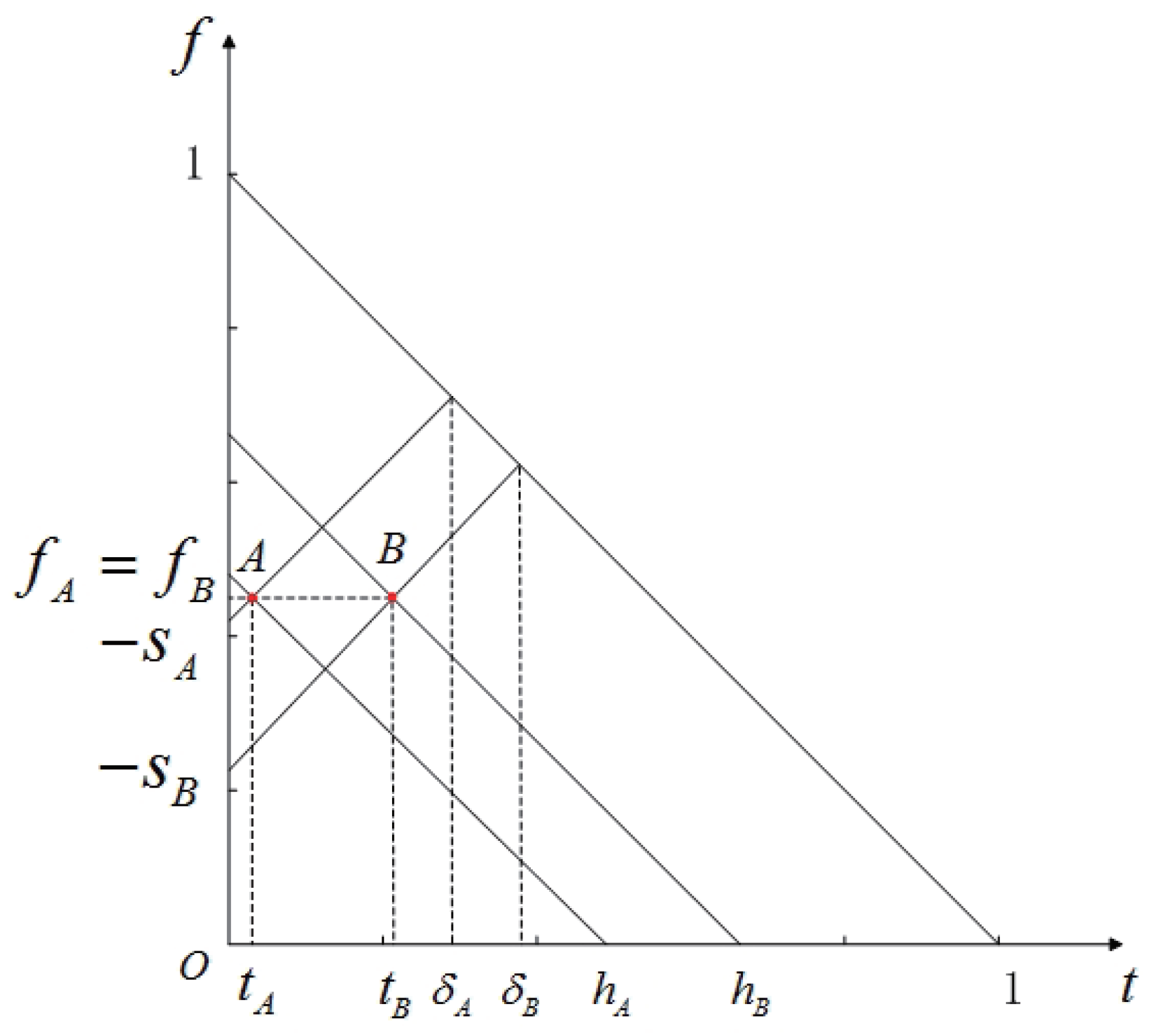
The results established in Theorem 6 and Corollary 3 indicate that the lexicographic orders
,
and
, in spite of being defined in terms of different measures, will always produce the same results when we use them to compare or rank IFVs. This equivalence is illustrated by
Figure 2.
It is worth noting that and are distinct lexicographic orders of IFVs as illustrated by the following example.
Example 2. Let and be two IFVs in . Then we have and . Thus it is clear that holds while is not true since and . In a similar fashion, we can prove that holds while is not true. Hence and are distinct.
According to Theorem 3, it follows that and are different. Using Corollary 1 and Corollary 3, a number of similar results can easily be deduced, which are no longer stated here. In addition, it should be noted that and are different lexicographic orders of IFVs as shown below.
Example 3. Let us consider two IFVsandIt is easy to see that and . Note first that since . On the other hand, is not true since . Similarly, we can prove that holds while is not true. This shows that and are distinct. From Corollary 2, it follows that and are different. Using Corollary 2 and Corollary 3, other similar results can easily be deduced, which are no longer stated here.
Motivated by Bustince’s ordering of intervals, we introduce the following order relations for IFVs.
Definition 27. Let and be IFVs in . The binary relation on is given by Definition 28. Let and be IFVs in . The binary relation on is given by Theorem 7. Let and be IFVs in . Then if and only if .
Proof. First, assume that . The following two cases should be considered.
(1) If , then .
(2) If
and
, we have
Thus
and
. That is,
.
Conversely, suppose that . Then we consider the following two cases.
(1) If , then .
(2) If
and
, we have
Thus
and
. That is,
. □
Theorem 8. Let and be IFVs in . Then the following are equivalent:
- (1)
;
- (2)
;
- (3)
;
- (4)
.
Proof. Note first that (1) and (4) are equivalent as shown in the proof of Theorem 7.
Next, we can also show that (1) and (2) are equivalent. In fact, suppose that
and
are two IFVs such that
and
. Then we have
Conversely, assume that
and
. Then we can deduce that
Thus (1) and (2) are equivalent.
Finally, it remains to prove that (1) and (3) are equivalent. To show this, assume first that
and
. Then we have
Conversely, assume that
and
. Then we can deduce that
Thus (1) and (3) are equivalent as well. This completes the entire proof of this theorem. □
Definition 29. Let and be IFVs in . The binary relation on is given by Definition 30. Let and be IFVs in . The binary relation on is given by Corollary 4. Let and be IFVs in . Then Proof. This follows directly from Theorem 8. □
The results established in Theorem 8 and Corollary 4 indicate that the lexicographic orders
,
,
and
, in spite of being defined in terms of different measures, will always produce the same results when we use them to compare or rank IFVs. This equivalence is illustrated by
Figure 3.
To complete our discussion, it suffices to show the differences among the rest of lexicographic orders of IFVs by several illustrative examples as follows.
Example 4. Consider two IFVsandIt is clear that and . Thus it follows that holds while is not true since and . Similarly, we can deduce that holds while is false. Therefore, and are distinct. From Theorem 3, it follows that and are different. Using Corollary 1 and Corollary 4, other similar results can easily be deduced, which are no longer stated here.
Example 5. Let and be two IFVs in . Thus it is clear that holds while is not true since and . Similarly, we can show that holds while is false. This shows that and are distinct.
According to Theorem 5, we can see that and are different as well. Using Corollary 3 and Corollary 4, other similar results can easily be deduced, which are no longer stated here.
Example 6. Consider two IFVsandSince and , it is clear that holds while is not true since and . In a similar fashion, it can be verified that is true while does not hold. Hence and are different. From Corollary 2, it follows that and are different. By virtue of Corollary 2 and Corollary 4, other similar results can easily be deduced, which are no longer stated here.
Theorem 9. The relation is an admissible order on .
Proof. First, we prove that is a linear order on . Let , be two IFVs in . Then the following four cases should be considered.
(1) If , then .
(2) If , then .
(3) If and , then .
(4) If and , then .
Thus we have either or for all . This means that is a linear order on .
Next, assume that
. Then we have
and
. Therefore, we can deduce that
If
, then
; otherwise, we have
and
, which also implies
.
Therefore, is an admissible order on . □
Theorem 10. The relation is an admissible order on .
Proof. The proof is similar to that of Theorem 9 and thus omitted. □
To summarize the discussion in this section, we demonstrate the relationships among thirteen lexicographic orders of IFVs with
Figure 4. Note that the meaning of the symbols or graphic elements used in
Figure 4 is as follows:
As shown in
Figure 4, all the lexicographic orders investigated in this section are admissible orders, which can be divided into four categories. The lexicographic orders from different categories are distinct in essence, while lexicographic orders in the same category are logically equivalent, in spite of being defined in terms of different measures.
5. Compatible Lexicographic Orders
Xu and Yager [
33,
37] initiated some fundamental operations for IFVs, which laid a solid foundation for aggregating intuitionistic fuzzy information.
Definition 31. [
37]
Let and be two IFVs in . Let λ be any positive real number. Then we have the following operations:;
.
In what follows, we refer to as the algebraic sum of the IFVs A and B. In addition, is called the scalar product of the positive real number and the IFV A.
Theorem 11. [
37]
Let and be two IFVs in . Let λ, and be positive real numbers. Then we have the following:- (1)
;
- (2)
;
- (3)
.
Definition 32. [
37]
Let () be IFVs in . The intuitionistic fuzzy weighted averaging (IFWA) operator of dimension n is a mapping given bywhere is the weight vector such that () and . Especially, if
, then
is simply written as
and called the
intuitionistic fuzzy averaging (IFA) operator. That is,
The following result is helpful for simplifying the calculation regarding IFWA operators.
Theorem 12. [
37]
Let (
)
. Then we havewhere is the weight vector. Proposition 1. Let and λ be any positive real number. Then we have the following:
- (1)
;
- (2)
;
- (3)
.
- (4)
.
Proof. Straightforward. □
Definition 33. Let ⪯ be a preorder on . Then we say that ⪯ is left compatible with the algebraic sum operation ifwhere , and are IFVs in . Definition 34. Let ⪯ be a preorder on . Then we say that ⪯ is right compatible with the algebraic sum operation ifwhere , and are IFVs in . A lexicographic order ⪯ is said to be compatible with the algebraic sum operation if it is both left and right compatible. Since the algebraic sum operation is commutative, we can immediately obtain the following result.
Proposition 2. Let ⪯ be a preorder on . Then the following statements are equivalent:
- (1)
⪯ is left compatible with the algebraic sum operation;
- (2)
⪯ is right compatible with the algebraic sum operation;
- (3)
⪯ is compatible with the algebraic sum operation.
Proof. Straightforward. □
Definition 35. Let ⪯ be a preorder on . Then we say that ⪯ is pseudo-compatible with the scalar product operation ifwhere and are positive real numbers. Definition 36. Let ⪯ be a preorder on . Then we say that ⪯ is compatible with the scalar product operation if it satisfies:
- (1)
;
- (2)
,
where and are positive real numbers.
Now, let us investigate whether the aforementioned lexicographic orders of IFVs are compatible with the algebraic sum operation.
Theorem 13. Let , and be IFVs in such that . Then we have the following:
- (1)
;
- (2)
;
- (3)
;
- (4)
;
- (5)
;
- (6)
.
Proof. Note that we only need to prove the first assertion. The others can be deduced from it using Corollary 3 and Theorem 11.
To show the first assertion, let us suppose that
holds. Then according to Definition 31, we have
and
Hence, we consider the following two cases:
(1) If
, we have
and so
.
(2) If
and
, then
and also we have
which means that
.
In both cases, we can deduce that . □
Proposition 3. Let , and be IFVs in with . Then Proof. By Definition 31, we have
and
Assume that and . Then the following two cases should be taken into account.
(1) If
, we have
and so
.
(2) If
and
, then
and we deduce that
That is,
.
In both cases, we can deduce that . □
It is worth noting that the condition cannot be removed in the above statement as demonstrated by the following example.
Example 7. Consider two IFVsandNote first that holds since . Let . By calculation, we have and . Thus it is clear thatsince and . This shows that is incompatible with the algebraic sum operation. Using Corollary 4, other similar results can be obtained for lexicographic orders , and , which are no longer stated here.
The following example shows that (or equivalently ) is not compatible with the algebraic sum operation.
Example 8. Consider two IFVsandNote first that and . Thus holds since . Let By calculation, we haveandSince , it follows thatThis shows that is incompatible with the algebraic sum operation. As shown below, is incompatible with the algebraic sum operation.
Example 9. Let us revisit the IFVs in Example 8. It is ease to see that holds since . Note also that holds since . This counterexample indicates that is not compatible with the algebraic sum operation of IFVs.
From Corollary 1, it follows that the lexicographic orders , and are incompatible with the algebraic sum operation of IFVs.
Theorem 14. Let . Then we have
- (1)
;
- (2)
,
where are positive real numbers.
Proof. Let and be two IFVs in . Let and be two positive real numbers. First, assume that . The following two cases should be considered.
(1) If
, then
, which implies that
(2) If
and
, then we have
and
In both cases, we can deduce that . This completes the proof of the first assertion.
Next, suppose that . If , it is clear that since is reflexive. Otherwise, let , and we consider the following three cases.
(1) If
, then
. It follows that
(2) If , then and so .
(3) If
, then
and we have
In all these cases, we can deduce that . This completes the proof of the second assertion. □
The above result shows that the lexicographic order is compatible with the scalar product operation. From Corollary 3, it follows that lexicographic orders and are compatible with the scalar product operation. In addition, we can prove the following result regarding the lexicographic order in a similar way.
Theorem 15. The lexicographic order is compatible with the algebraic sum operation of IFVs.
Proof. Let and be two IFVs in . Let and be two positive real numbers. First, assume that . The following two cases should be considered.
(1) If
, then we have
(2) If
and
, then we have
and
since
.
In both cases, we can deduce that . This completes the proof of the first assertion.
Next, suppose that . If , it is clear that since is reflexive. Otherwise, let , and the following three cases should be considered.
(1) If
, then we have
(2) If , then and so .
(3) If
, then
and we have
since
.
In all these cases, we can deduce that . This completes the proof of the second assertion. □
From Corollary 4 and the above result, it follows that , and are compatible with the scalar product operation.
Example 10. Consider two IFVsandNote that since and . On the other hand, we haveandSince , it is clear that . This counterexample shows that the lexicographic order is incompatible with the scalar product operation. Nevertheless, the following result shows that is pseudo-compatible with the scalar product operation.
Theorem 16. Let . Then we havewhere are positive real numbers. Proof. Let be an IFV in . Let and be two positive real numbers such that . If , then since is reflexive. Otherwise, let , and we consider the following three cases.
(1) If
, then
. Note also that
Thus we can deduce that
which implies that
.
(2) If , then and so .
(3) If
, then
. It follows that
If
, the result follows directly. Otherwise, we have
, which implies that
, and so
.
In all these cases, we can deduce that . This completes the proof. □
Using Corollary 1, other similar results can be obtained for lexicographic orders , and , which are no longer stated here.
Example 11. Consider two IFVsandSince and , we have . Taking , we have and . It follows that since . This shows that (or equivalently ) is incompatible with the scalar product operation. It is worth noting that (or equivalently ) is pseudo-compatible with the scalar product operation as shown below.
Theorem 17. Let . Then we havewhere are positive real numbers. Proof. The proof is similar to that of Theorem 16 and thus omitted. □
At the end of this section, we summarize various compatible properties of different lexicographic orders in
Table 1. For the sake of convenience, we choose only one particular order as the representative in each distinct category of lexicographic orders (see
Figure 4). Note also that the full terms corresponding to the acronyms in
Table 1 are given below:
CAS stands for compatibility with the algebraic sum operation;
CSP stands for compatibility with the scalar product operation;
PCSP stands for pseudo-compatibility with the scalar product operation.
From
Table 1, we can see that all the lexicographic orders discussed in the previous section are pseudo-compatible with the scalar product operation. The orders
and
are compatible with the scalar product. It is worth noting that the order
is the only lexicographic order which satisfies all the compatible properties. In this sense, the order
can perfectly serve the purpose of ranking IFVs in cooperation with the IFWA operator.
6. Numerical Illustration
To demonstrate the practical value of the theoretical results obtained in previous sections, we revisit a benchmark problem regarding risk investment, which was originally raised by Herrera and Herrera-Viedma [
52]. Later on, Wei [
53] considered the same problem in an intuitionistic fuzzy setting. This problem was further investigated by Chen and Tu in [
34]. Note that a similar problem was discussed by Wu and Chen [
54] as well.
Assume that there is an investment bank B which intends to invest a sum of money to the most appropriate company. Let us denote by U the collection of five companies under the consideration of the bank B. Specifically, the alternatives in U for potential investment include:
In order to choose the most suitable company, a committee consisting of ten experts is organized by the bank B to give the evaluation of all companies according to four criteria in . The meaning of the criterion () is as follows:
stands for low investment risk;
stands for high growth rate;
stands for positive social-political impact;
stands for low environmental pollution.
All these criteria are beneficial ones. To facilitate the comparison, the evaluation results are inherited verbatim from [
53]. These results can be described by an intuitionistic fuzzy soft set
over
U, as shown in
Table 2. For instance, the assessment result of the company
with respect to the criterion
is given by the IFV
. This can be interpreted as “four experts in the committee think that the food company causes low environmental pollution, while five experts disagree with this opinion, and also there is one expert who declines to give his/her opinion on this issue”.
Following the way of discussion in [
53], we consider the following two different cases. In both cases, the IFWA operator will be used to aggregate the concerned intuitionistic fuzzy information.
Case 1: In this case, the information about the attribute weights is partly known and the weights can be determined by solving the following single-objective programming model, as established in [
53].
The obtained weight vector is
Using this weight vector, we can calculate the aggregated intuitionistic fuzzy preference value (AIFPV)
(
) as follows:
For instance, the AIFPV
can be obtained by
Moreover, we calculate the score of the AIFPVs. For instance, we have
. Other results regarding the AIFPVs and related measures can be found in
Table 3. In addition, the ranking results of five companies respectively based on the lexicographic orders
,
,
and
are shown in
Table 4.
There are several important points need to be mentioned in view of the results obtained in Case 1:
Firstly, note that the ranking results given by the orders
and
are identical, since the scores
(
) are all different. In such a particular situation, the orders
and
will definitely produce the same ranking result as only the score function is used indeed. Nevertheless, it should be noted that
and
are not logically equivalent in general as shown in
Section 4.
Secondly, recall that Wei [
53] ranked the companies
(
) by means of the order
. The result is as follows:
which is the same as the result given by the order
in
Table 4. In fact, we assert that the orders
and
will always produce the same ranking, because they are logically equivalent according to Corollary 1. It is worth noting that the IFWA operator and the order
was jointly utilized to aggregate the IFVs and rank the alternatives in [
53]. Nevertheless, as mentioned in
Section 5, the order
(or equivalently
) is only pseudo-compatible with the scalar product operation. As illustrated by Example 10, it might happen that
and meanwhile
for
in some cases. Consequently, the order
might give rise to unreasonable ranking results since it is difficult to act perfectly in cooperation with the IFWA operator.
Last but not least, as pointed out in
Section 5, the order
is an admissible order on
which is compatible with both the algebraic sum and scalar product operations. Thus the order
is able to rank IFVs jointly with the IFWA operator in a perfect manner. As a result, the ranking result given by the order
is more reasonable indeed, even though it looks quite different from the results given by other orders in Case 1.
In fact, the orders and might occasionally produce the same ranking result in some other cases. This will be further illustrated in the discussion below.
Case 2: In this case, the information about the attribute weights is completely unknown. For the sake of convenience, we assume that each attribute has the equal weight. That is, the weight vector is
Note that some minor changes are made to the evaluation regarding the company
. The new evaluation information can be expressed by another intuitionistic fuzzy soft set
over
U, as shown in
Table 5.
Based on the intuitionistic fuzzy soft set
and new weight vector
, we can calculate the corresponding AIFPVs and related measures as done in Case 1. The results are shown in
Table 6. Moreover, the ranking results of five companies respectively based on the lexicographic orders
,
,
and
are shown in
Table 7.
We would like to point out the following two issues regarding the results obtained in Case 2.
Firstly, unlike in Case 1, the ranking results given by the orders
and
become different in this case. Specifically, the result given by
is
while the result given by
is
since
,
and
.
Secondly, recall that the ranking result given by the order
is different from the results given by other orders in Case 1. However, in this case, it is interesting to observe that the orders
and
can by chance bring forth the same ranking results:
even though they are distinct in essence as revealed in
Section 4.
Remark 1. To summarize the discussion in above two cases, we conclude that the lexicographic order (or equivalently and ) is most suitable for ranking IFVs in those intuitionistic fuzzy multiple attribute decision making procedures, where IFWA operator are utilized to aggregate the original decision information quantified in terms of IFVs. This is mainly due to the fact that is compatible with both the algebraic sum and scalar product operations. Thus it can cooperate with the IFWA operator and serve the purpose of ranking IFVs in a coordinated way. On the other hand, if other lexicographic orders such as , or will be used in intuitionistic fuzzy multiple attribute decision making, we should consider replacing the IFWA operator with other aggregation operators, which are consistent with the selected lexicographic order.


