An Interval Type-2 Fuzzy Similarity-Based MABAC Approach for Patient-Centered Care

Abstract

Patient-centered care is an essential part of the implementation of integrated medicine, integrating humanistic care into nursing services, enhancing communication between caregivers and patients, and providing personalized service to patients. Based on the similarity of interval type-2 fuzzy numbers (IT2FNs), a novel similarity-based methodology is presented for the selection of the most suitable medical treatment under a patient-centered environment. First, we propose a new similarity based on the geometric properties of interval type-2 fuzzy numbers and present a new property based on the center of gravity. Meanwhile, in order to better highlight the advantages of the proposed similarity, we selected 30 samples for comparative experiments. Second, considering the straightforward logic of the multi-attributive border approximation area comparison (MABAC) method, we extended it based on similarity to make the decision more accurate. Finally, a realistic patient-centered type-2 diabetes treatment selection problem is presented to verify the practicality and effectiveness of the proposed algorithm. A comparative analysis with existing methods is also described.

1. Introduction

With the advancement of human society and medical technology, the medical service mode of disease-centered care has been gradually replaced by patient-centered care (PCC). Patient-centered care can provide patients with a full range of quality services in a variety of ways, including physical, psychological, and social needs [1,2] by satisfying and responding the patient's wants, needs, and preferences, allowing patients to participate in decision-making of their own treatment and care [3]. As Steiger and Balog [4] point out, PCC treats the patient as a unique individual, places the patient in the center of the care process, and takes into account the patient’s beliefs and values, as well as physical and emotional needs [5,6]. PCC provides patients with plenty of opportunities to participate in decision-making, that is, to assume that the patient can quantify their needs and make decisions that meet their specific needs and wants [7]. However, it is difficult to provide patients with appropriate advice so that they can make decisions easily. First, the degree of the patient's involvement in decision-making is highly inconsistent [8]. Some patients are willing to participate actively in discussions on treatment options, but others are more dependent on the decision of the attending physician. Second, despite the active participation of patients, the patient's medical skills and knowledge is not enough to support them to make a decision by themselves, but may delay the treatment of the disease [9]. Third, in the process of patient-centered decision-making, there are many restrictions here, such as the subjective ambiguity of the patient, uncertainty of the decision-making environment, and the complexity of objective things. Hence, it is not adequate to determine the values with a certain number. Instead, it is easy to express the linguistic assessment values using interval type-2 fuzzy numbers (IT2FNs) [10,11].

In real life, decision makers (DMs) prefer to use linguistic terms to explain the criteria of various kinds of alternatives [12,13,14,15,16,17]. Zadeh [18] put forward a new concept called linguistic variables, which can correspond to different fuzzy sets, such as triangular fuzzy numbers, intuitionistic fuzzy numbers, interval type-2 fuzzy sets, etc. The concept of linguistic variables can effectively be applied to deal with complicated or unexplained situations and are frequently represented by type-2 fuzzy sets [19]. The general type-2 fuzzy numbers (GT2FNs) have been around for decades as one of the major areas in the field of fuzzy sets [20]. This is because many applications in the use of GT2FNs have a strong performance, compared to other fuzzy sets [21]. For example, GT2FNs are most widely applied to the fuzzy recognition, decision making, knowledge classification, medical diagnosis, clustering, control systems, databases, and so on [22,23,24,25,26,27,28,29]. With regard to patient-centered decision-making, it is not easy for patients to express the subjective ideas of the medical care. Therefore, it is better to represent a higher order fuzzy set rather than an exact membership grade. Wei and Chen [30] extended the GT2FNs to IT2FNs, giving the decision maker greater freedom to take the decision. Moreover, the primary and secondary functions of IT2FNs can express uncertain information more accurately and have lower computational complexity than GT2FNs. Therefore, many studied have focused on the research topic of IT2FNs [31,32,33,34]. In our study, IT2FNs are applied to develop the new algorithm to solve the medical treatment selection decision-making problem in a patient-centered environment.

In recent years, a lot of researchers have proposed various methods to expand the degree of similarity between fuzzy numbers [35,36,37,38,39,40]. However, these similarity measures have their own shortcomings, such as the results do not agree with intuition, or the results cannot calculate for the denominator when it is equal to 0. Due to this situation, in this paper, based on the difference of proportion, geometric distance, height, and center-of-gravity distance of two interval type-2 fuzzy numbers, we developed a new similarity measure within an interval type-2 fuzzy environment. Then, we confirmed the basic properties and proposed a new property that is based the center of gravity. Next, comparative analysis of 30 different sets of generalized type-2 fuzzy numbers was conducted, and its results prove the superiority of the proposed similarity measure. Finally, the proposed similarity measure is used to handle the medical treatment options selection problem in interval type-2 fuzzy environment.

Pamučar and Ćirović [41] proposed the multi-attributive border approximation area comparison (MABAC) method in 2015, which has a straightforward computation procedure and expresses the systematic and logical decision theory. Furthermore, the MABAC method subsequently was further developed in References [42,43,44], which applied the MABAC method for material selection problems under interval-valued intuitionistic fuzzy environments. Peng and Yang [44] presented a new approach to R&D project selection problems to find the best project based on both Pythagorean fuzzy sets and MABAC. As far as we know, the studies of the MABAC methods are few. This paper proposes a similarity-based MABAC approach under the interval type-2 fuzzy numbers.

In recent years, there are many similarity-based multiple criteria decision making (MCDM) methods, such as References [45,46], which can improve the method’s flexibility. Until now, related studies of similarity-based MABAC method under an interval type-2 fuzzy numbers environment have been not seen. Therefore, paying attention to this aspect is a meaningful subject. Therefore, we focus our attention on extending the MABAC method to accommodate the interval type-2 fuzzy environment and look at their application to medical treatment selection problems in this paper. Then, we summarize the motives and contributions of this paper as follows:

• There are several motivations for using IT2FNs. First, common fuzzy numbers, such as triangular fuzzy numbers and generalized type-2 fuzzy numbers, have some limitations regarding directly dealing with uncertain information. In practical applications, the same linguistic term may represent different meanings for different people. IT2FNs give DMs greater freedom in the determination of the membership function, and it can better describe and deal with inaccurate information. Second, compared with GT2FNs, IT2FNs have lower computational complexity. Therefore, IT2FNs is applied to develop the new algorithm to solve the medical treatment selection decision-making problem in a patient-centered environment.
• Considering the existing interval type-2 fuzzy similarity measures, there are some limitations for some particular sets. Therefore, we propose a new similarity, which represents the degree of closeness between two IT2FNs. Moreover, we not only present a new property of the similarity measure, but it also overcomes the drawback of other existing interval type-2 fuzzy similarity measures. Through a large number of comparative experiments, the advantages of the proposed interval type-2 fuzzy similarity are confirmed. Thereby, the proposed similarity algorithm is more scientific and effective.
• Due to the computational complexity of the interval type-2 fuzzy similarity, we need a simpler and more straightforward approach to making decisions. Compared to other decision-making methods, MABAC is more simplified and straightforward. MABAC is applied to solve the computational complexity of IT2FNs and interval type-2 fuzzy similarity, which is helpful to improve the performance of the interval type-2 fuzzy similarity in practice. Moreover, in order to optimize the composition of the proposed algorithm and improve the efficiency and accuracy of the calculation process, we propose a similarity-based MABAC method. The proposed method is less complex and more straightforward than the other methods.

The remainder of this paper is organized as follows. In Section 2, we briefly introduce the definition of GT2FNs, IT2FNs, and their arithmetic. In Section 3, we present a new similarity measure and extend it in IT2FNs. Furthermore, we also prove a new property of the new similarity measure. Finally, we use thirty sets of GT2FNs to make a comparison with the existing similarity measures. In Section 4, based on the proposed similarity, the MABAC approach is developed under interval type-2 fuzzy environments. In Section 5, we introduce a procedure for the patient-centered care problem based on the modified MABAC method. Then, we use a real treatment selection problem to illustrate the proposed method and compare it with other existing methods. Finally, the conclusions are discussed in Section 6.

2. Preliminaries

In this section, we briefly introduce the concept of generalized type-2 fuzzy set (GT2FS) and IT2FNs. Then, we review the arithmetic operations between interval type-2 fuzzy numbers.

Definition 1

[24]. A GT2FS $\tilde{A}$ in the universe of discourse can be denoted by its membership function ${\mu }_{\tilde{A}}\left(x\right)$, where $x\in X$, $u\in J_x\subseteq \left[0,1\right]$ and $0\le {\mu }_{\tilde{A}}\left(x\right)\le 1$, and $\tilde{A}$ is given as follows:

$$\tilde{A}=\left\{\left(\left(x,u\right),{\mu }_{\tilde{A}}\left(x,u\right)|\forall x\in X,\forall u\in J_x\subseteq \left[0,1\right]\right)\right\}.$$

If $\tilde{A}$ is continuous, it also can be expressed as:

$$\tilde{A}=\left\{{\displaystyle {\int }_{x\in X}\frac{{\mu }_{\tilde{A}}\left(x\right)}{x}}\right\}=\left\{{\displaystyle {\int }_{x\in X}{\displaystyle {\int }_{u\in J_{x\subseteq \left[0,1\right]}^u}\frac{{\mu }_{\tilde{A}}\left(x\right)}{x}}}\right\}=\left\{\frac{{\displaystyle {\int }_{x\in X}\left[{\displaystyle {\int }_{u\in J_{x\subseteq \left[0,1\right]}^u}\frac{f_x\left(x,u\right)}{u}}\right]}}{x}\right\},$$

where$\int \int$represents the union for$x$and$u$, and$J_x$is called the primary membership of$x$in$\tilde{A}$.

If${\mu }_{\tilde{A}}\left(x\right)=1$for$\forall x\in X$,$\tilde{A}$is called an interval type-2 fuzzy set (IT2FS) and represented by:

$$\tilde{A}=\left\{\left(\left(x,u\right),{\mu }_{\tilde{A}}\left(x,u\right)=1|\forall x\in X,\forall u\in J_x\subseteq \left[0,1\right]\right)\right\}.$$

Definition 2

[47]. Let $\tilde{A}$ be an IT2FS in the universe of discourse $X$ and $U$, where $\tilde{A}$ is equal to the union of all its embedded T2FSs ${\tilde{A}}_e^j$. An embedded T1FS $A_e^j$ is the domain of each ${\tilde{A}}_e^j$, and $\tilde{A}$ can therefore be expressed as follows:

$$\tilde{A}=1/{\displaystyle \underset{j=1}{\overset{n_A}{\cup }}{A}_e^j},$$

where $n_A$ is the number of embedded T1FS $A_e^j$. For convenience, $\tilde{A}$ can be denoted as $\tilde{A}={\displaystyle {\cup }_{i=1}^n{A}_i}$, where $A_i$ is an embedded T1FS. When $X$ has only one element, IT2FS $\tilde{A}$ is reduced to interval type-2 fuzzy numbers (IT2FNs).

Definition 3

[48]. Let $\tilde{\tilde{A}}$ be an IT2FNs, which can be represented as follows:

$$\tilde{\tilde{A}}=\left[{\tilde{\tilde{A}}}^L,{\tilde{\tilde{A}}}^U\right]=\left[\left(a_1^L,a_2^L,a_3^L,a_4^L;w_{{\tilde{\tilde{A}}}^L}\right),\left(a_1^U,a_2^U,a_3^U,a_4^U;w_{{\tilde{\tilde{A}}}^U}\right)\right].$$

$\tilde{\tilde{A}}$ is shown in Figure 1, where $0\le a_1^L\le a_2^L\le a_3^L\le a_4^L\le 1$, $0\le a_1^U\le a_2^U\le a_3^U\le a_4^U\le 1$, $0\le w_{{\tilde{\tilde{A}}}^L}\le w_{{\tilde{\tilde{A}}}^U}\le 1$, $w_{{\tilde{\tilde{A}}}^U}\ne 0$, and ${\tilde{\tilde{A}}}^L\subset {\tilde{\tilde{A}}}^U$. Figure 1 shows that interval type-2 fuzzy number $\tilde{\tilde{A}}$ is composed of two type-2 fuzzy numbers ${\tilde{\tilde{A}}}^L$ and ${\tilde{\tilde{A}}}^U$, where ${\tilde{\tilde{A}}}^L$ is referred to as the lower type-2 fuzzy number and ${\tilde{\tilde{A}}}^U$ is referred to as the upper type-2 fuzzy number.

Suppose there are two interval-valued fuzzy numbers $\tilde{\tilde{A}}$ and $\tilde{\tilde{B}}$, denoted as

$$\tilde{\tilde{A}}=\left[{\tilde{\tilde{A}}}^L,{\tilde{\tilde{A}}}^U\right]=\left[\left(a_1^L,a_2^L,a_3^L,a_4^L;w_{{\tilde{\tilde{A}}}^L}\right),\left(a_1^U,a_2^U,a_3^U,a_4^U;w_{{\tilde{\tilde{A}}}^U}\right)\right]$$

and

$$\tilde{\tilde{B}}=\left[{\tilde{\tilde{B}}}^L,{\tilde{\tilde{B}}}^U\right]=\left[\left(b_1^L,b_2^L,b_3^L,b_4^L;w_{{\tilde{\tilde{B}}}^L}\right),\left(b_1^U,b_2^U,b_3^U,b_4^U;w_{{\tilde{\tilde{B}}}^U}\right)\right],$$

where $0\le a_1^L\le a_2^L\le a_3^L\le a_4^L\le 1$, $0\le a_1^U\le a_2^U\le a_3^U\le a_4^U\le 1$, $0\le b_1^L\le b_2^L\le b_3^L\le b_4^L\le 1$, and $0\le b_1^U\le b_2^U\le b_3^U\le b_4^U\le 1$. Then, by Reference [49], the operational laws between the interval type-2 fuzzy numbers $\tilde{\tilde{A}}$ and $\tilde{\tilde{B}}$ are defined as follows:

(1) Interval type-2 fuzzy numbers addition operation:

$$\begin{gathered} \stackrel{\approx }{A}\oplus \stackrel{\approx }{\mathrm{B}}=\left[\left(a_1^L,a_2^L,a_3^L,a_4^L;w_{\stackrel{\approx }{A^L}}\right),\left(a_1^U,a_2^U,a_3^U,a_4^U;w_{\stackrel{\approx }{A^U}}\right)\right] \\ \oplus \left[\left(b_1^L,b_2^L,b_3^L,b_4^L;w_{\stackrel{\approx }{B^L}}\right),\left(b_1^U,b_2^U,b_3^U,b_4^U;w_{\stackrel{\approx }{B^U}}\right)\right] \\ =[\left(a_1^L+b_1^L-a_1^L{b}_1^L,a_2^L+b_2^L-a_2^L{b}_2^L,a_3^L+b_3^L-a_3^L{b}_3^L,a_4^L+b_4^L-a_4^L{b}_4^L;\min \left(w_{\stackrel{\approx }{A^L}},w_{\stackrel{\approx }{B^L}}\right)\right), \\ \left(a_1^U+b_1^U-a_1^U{b}_1^U,a_2^U+b_2^U-a_2^U{b}_2^U,a_3^U+b_3^U-a_3^U{b}_3^U,a_4^U+b_4^U-a_4^U{b}_4^U;\min \left(w_{\stackrel{\approx }{A^U}}{w}_{\stackrel{\approx }{B^U}}\right)\right)]. \end{gathered}$$

(2) Interval type-2 fuzzy numbers subtraction operation:

$$\begin{gathered} \begin{array}{l}\stackrel{\approx }{A}\mathsf{\Theta }\stackrel{\approx }{\mathrm{B}}=\left[\left(a_1^L,a_2^L,a_3^L,a_4^L;w_{\stackrel{\approx }{A^L}}\right),\left(a_1^U,a_2^U,a_3^U,a_4^U;w_{\stackrel{\approx }{A^U}}\right)\right]\\ \mathsf{\Theta }\left[\left(b_1^L,b_2^L,b_3^L,b_4^L;w_{\stackrel{\approx }{B^L}}\right),\left(b_1^U,b_2^U,b_3^U,b_4^U;w_{\stackrel{\approx }{B^U}}\right)\right]\end{array} \\ =[\left(a_1^L-b_1^L,a_2^L-b_2^L,a_3^L-b_3^L,a_4^L-b_4^L;\min \left(w_{\stackrel{\approx }{A^L}},w_{\stackrel{\approx }{B^L}}\right)\right),\left(a_1^U-b_1^U,a_2^U-b_2^U,a_3^U-b_3^U,a_4^U-b_4^U;\min \left(w_{\stackrel{\approx }{A^U}}{w}_{\stackrel{\approx }{B^U}}\right)\right)]. \end{gathered}$$

(3) Interval type-2 fuzzy numbers multiplication operation:

$$\begin{gathered} \begin{array}{l}\stackrel{\approx }{A}\otimes \stackrel{\approx }{\mathrm{B}}=\left[\left(a_1^L,a_2^L,a_3^L,a_4^L;w_{\stackrel{\approx }{A^L}}\right),\left(a_1^U,a_2^U,a_3^U,a_4^U;w_{\stackrel{\approx }{A^U}}\right)\right]\\ \otimes \left[\left(b_1^L,b_2^L,b_3^L,b_4^L;w_{\stackrel{\approx }{B^L}}\right),\left(b_1^U,b_2^U,b_3^U,b_4^U;w_{\stackrel{\approx }{B^U}}\right)\right]\end{array} \\ =\left[\left(a_1^L{b}_1^L,a_2^L{b}_2^L,a_3^L{b}_3^L,a_4^L{b}_4^L;\min \left(w_{\stackrel{\approx }{A^L}},w_{\stackrel{\approx }{B^L}}\right)\right),\left(a_1^U{b}_1^U,a_2^U{b}_2^U,a_3^U{b}_3^U,a_4^U{b}_4^U;\min \left(w_{\stackrel{\approx }{A^U}},w_{\stackrel{\approx }{B^U}}\right)\right)\right] \end{gathered}$$

(4) Interval type-2 fuzzy numbers division operation:

$$\begin{gathered} \begin{array}{l}\stackrel{\approx }{A}\varnothing \stackrel{\approx }{\mathrm{B}}=\left[\left(a_1^L,a_2^L,a_3^L,a_4^L;w_{\stackrel{\approx }{A^L}}\right),\left(a_1^U,a_2^U,a_3^U,a_4^U;w_{\stackrel{\approx }{A^U}}\right)\right]\\ \varnothing \left[\left(b_1^L,b_2^L,b_3^L,b_4^L;w_{\stackrel{\approx }{B^L}}\right),\left(b_1^U,b_2^U,b_3^U,b_4^U;w_{\stackrel{\approx }{B^U}}\right)\right]\end{array} \\ =[\left(a_1^L/b_4^L,a_2^L/b_3^L,a_3^L/b_2^L,a_4^L/b_1^L;\min \left(w_{\stackrel{\approx }{A^L}},w_{\stackrel{\approx }{B^L}}\right)\right), \\ \left(a_1^U/b_4^U,a_2^U/b_3^U,a_3^U/b_2^U,a_4^U/b_1^U;\min \left(w_{\stackrel{\approx }{A^U}},w_{\stackrel{\approx }{B^U}}\right)\right)] \end{gathered}$$

where

$$a/b=\{\begin{array}{l}\frac{a}{b},\mathrm{if}\mathrm{a}\text{<}\mathrm{b},\\ 1,\mathrm{otherwise}.\end{array}$$

Definition 4

[50]. An interval type-2 fuzzy number can be represented as $\stackrel{\approx }{A}=\left[\stackrel{\approx }{A^L},\stackrel{\approx }{A^U}\right]=\left[\left(a_1^L,a_2^L,a_3^L,a_4^L;w_{\stackrel{\approx }{A^L}}\right),\left(a_1^U,a_2^U,a_3^U,a_4^U;w_{\stackrel{\approx }{A^U}}\right)\right]$ $\left(i=1,2,\dots ,n\right)$, and $p,q\ge 0$, then the aggregation function given as:

$$ITFGB{M}^{p,q}\left(\stackrel{\approx }{A_1},\stackrel{\approx }{A_2},\dots ,\stackrel{\approx }{A_n}\right)=\frac{1}{p+q}{\left(\underset{\begin{array}{l}i,j=1\\ i\ne j\end{array}}{\overset{n}{\otimes }}\left(p\stackrel{\approx }{A_i}\oplus q\stackrel{\approx }{A_j}\right)\right)}^{1/n(n-1)}$$

(1)

is called the interval type-2 fuzzy geometric Bonferroni mean (ITFGBM) operator.

3. New Similarity Measures for Interval Type-2 Fuzzy Numbers

3.1. The New Similarity Measures

In this section, we present a new similarity measure between GT2FNs and IT2FNs. This method combines the concept of geometric distance, the center of gravity (COG) distance, proportion, and height of a type-2 fuzzy number.

Definition 5.

Let$\stackrel{\sim }{A}=\left(a_1,a_2,a_3,a_4;w_{\stackrel{\sim }{A}}\right)$and$\stackrel{\sim }{B}=\left(b_1,b_2,b_3,b_4;w_{\stackrel{\sim }{B}}\right)$be two generalized type-2 fuzzy numbers, then the similarity between these two fuzzy numbers, is defined as:

$$S(\stackrel{\sim }{A},\stackrel{\sim }{B})=\left(1-\frac{1}{8}{\displaystyle \sum _{i=1}^4\left|a_i-b_i\right|}-\frac{d(A^{\ast },B^{\ast })}{2}\right)\times \left(1-\frac{1}{2}\times \left(\left|pr(\stackrel{\sim }{A})-pr(\stackrel{\sim }{B})\right|+\left|w_{\stackrel{\sim }{A}}-w_{\stackrel{\sim }{B}}\right|\right)\right),$$

(2)

where

$$pr(\stackrel{\sim }{A})=\frac{(a_4+a_3-a_2-a_1)\times w_{\stackrel{\sim }{A}}}{2},$$

$$\begin{gathered} pr(\stackrel{\sim }{B})=\frac{(b_4+b_3-b_2-b_1)\times w_{\stackrel{\sim }{B}}}{2}, \\ d({\stackrel{\sim }{A}}^{\ast },{\stackrel{\sim }{B}}^{\ast })=\frac{\sqrt{{(x_{{\stackrel{\sim }{A}}^{\ast }}-x_{{\stackrel{\sim }{B}}^{\ast }})}^2+{(y_{{\stackrel{\sim }{A}}^{\ast }}-y_{{\stackrel{\sim }{B}}^{\ast }})}^2}}{\sqrt{1.25}}, \\ {y}_{{\stackrel{\sim }{A}}^{}}^{\ast }=\{\begin{array}{l}\frac{{\displaystyle w_{\stackrel{\sim }{A}}}\times \left(\frac{a_3^{}-a_2^{}}{a_4^{}-a_1^{}}+2\right)}{6}\mathrm{if}{a}_1^{}\ne a_4^{}\mathrm{and}0<w_{\stackrel{\sim }{A}}^{}\le 1,\\ \frac{W_{\stackrel{\sim }{A}}^{}}{2},\mathrm{if}{a}_1^{}=a_4^{}\mathrm{and}0<w_{\stackrel{\sim }{A}}^{}\le 1,\end{array} \\ {x}_{{\stackrel{\sim }{A}}^{}}^{\ast }=\{\begin{array}{l}\frac{y_{{\stackrel{\sim }{A}}^{}}^{\ast }\left(a_3^{}+a_2^{}\right)+\left(a_4^{}+a_1^{}\right)\left(w_{\stackrel{\sim }{A}}^{}-y_{{\stackrel{\sim }{A}}^{}}^{\ast }\right)}{2w_{\stackrel{\sim }{A}}^{}}{\mathrm{if}w}_{\stackrel{\sim }{A}}\ne 0,\\ \frac{a_4+a_1}{2}{\mathrm{if}w}_{\stackrel{\sim }{A}}=0,\end{array} \\ {y}_{{\stackrel{\sim }{B}}^{}}^{\ast }=\{\begin{array}{l}\frac{w_{\stackrel{\sim }{B}}^{}\times \left(\frac{b_3^{}-b_2^{}}{b_4^{}-b_1^{}}+2\right)}{6}\mathrm{if}{b}_1^{}\ne b_4^{}\mathrm{and}0<w_{\stackrel{\sim }{B}}^{}\le 1,\\ \frac{W_{\stackrel{\sim }{B}}^{}}{2},\mathrm{if}{b}_1^{}=b_4^{}\mathrm{and}0<w_B^{}\le 1,\end{array} \\ {x}_{{\stackrel{\sim }{B}}^{}}^{\ast }=\{\begin{array}{l}\frac{y_{{\stackrel{\sim }{B}}^{}}^{\ast }\left(b_3^{}+b_2^{}\right)+\left(b_4^{}+b_1^{}\right)\left(w_{\stackrel{\sim }{B}}^{}-y_{{\stackrel{\sim }{B}}^{}}^{\ast }\right)}{2w_{\stackrel{\sim }{B}}^{}}{\mathrm{if}w}_{\stackrel{\sim }{B}}\ne 0,\\ \frac{b_4+b_1}{2}{\mathrm{if}w}_{\stackrel{\sim }{B}}=0.\end{array} \end{gathered}$$

Definition 6.

Let$\stackrel{\approx }{A}=\left[\stackrel{\approx }{A^L},\stackrel{\approx }{A^U}\right]=\left[\left(a_1^L,a_2^L,a_3^L,a_4^L;w_{\stackrel{\approx }{A^L}}\right),\left(a_1^U,a_2^U,a_3^U,a_4^U;w_{\stackrel{\approx }{A^U}}\right)\right]$and$\stackrel{\approx }{B}=\left[\stackrel{\approx }{B^L},\stackrel{\approx }{B^U}\right]=\left[\left(b_1^L,b_2^L,b_3^L,b_4^L;w_{\stackrel{\approx }{B^L}}\right),\left(b_1^U,b_2^U,b_3^U,b_4^U;w_{\stackrel{\approx }{B^U}}\right)\right]$be two interval type-2 fuzzy numbers, where$0\le a_1^L\le a_2^L\le a_3^L\le a_4^L\le 1$,$0\le a_1^U\le a_2^U\le a_3^U\le a_4^U\le 1$,$0\le b_1^L\le b_2^L\le b_3^L\le b_4^L\le 1$, and$0\le b_1^U\le b_2^U\le b_3^U\le b_4^U\le 1$. Based on Equation (2), the lower fuzzy similarity$S\left(\stackrel{\approx }{A^L},\stackrel{\approx }{B^L}\right)$and the upper similarity$S\left(\stackrel{\approx }{A^U},\stackrel{\approx }{B^U}\right)$are calculated. Then, the new similarity measures of two interval type-2 fuzzy numbers can be calculated as follows:

$$S(\stackrel{\approx }{A^{}},\stackrel{\approx }{B^{}})=\sqrt{S(\stackrel{\approx }{A^L},\stackrel{\approx }{B^L})\times S(\stackrel{\approx }{A^U},\stackrel{\approx }{B^U})}$$

(3)

where

$$S(\stackrel{\approx }{A^L},\stackrel{\approx }{B^L})=\left(1-\frac{1}{8}{\displaystyle \sum _{i=1}^4\left|a_i^L-b_i^L\right|}-\frac{d(A^L{}^{\ast },B^L{}^{\ast })}{2}\right)\times \left(1-\frac{1}{2}\left\{\left|pr(\stackrel{\approx }{A^L})-pr(\stackrel{\approx }{B^L})\right|+\left|w_{\stackrel{\approx }{A^L}}-w_{\stackrel{\approx }{B^L}}\right|\right\}\right),$$

(4)

$$S(\stackrel{\approx }{A^U},\stackrel{\approx }{B^U})=\left(1-\frac{1}{8}{\displaystyle \sum _{i=1}^4\left|a_i^U-b_i^U\right|}-\frac{d(A^U{}^{\ast },B^U{}^{\ast })}{2}\right)\times \left(1-\frac{1}{2}\left\{\left|pr(\stackrel{\approx }{A^U})-pr(\stackrel{\approx }{B^U})\right|+\left|w_{\stackrel{\approx }{A^U}}-w_{\stackrel{\approx }{B^U}}\right|\right\}\right).$$

(5)

Now, some properties of this presented similarity measure between interval-valued fuzzy numbers are deduced as follows:

Property 1.

$S\left(\stackrel{\approx }{A},\stackrel{\approx }{B}\right)=1$if and only if$\stackrel{\approx }{A}=\stackrel{\approx }{B}$.

Proof. 

When $\stackrel{\approx }{A}=\stackrel{\approx }{B}$, there are $a_i^L=b_i^L$, $a_i^U=b_i^U$, $w_{\stackrel{\approx }{A^L}}=w_{\stackrel{\approx }{B^L}}$, and $w_{\stackrel{\approx }{A^U}}=w_{\stackrel{\approx }{B^U}}$. Then, there are $pr\left(\stackrel{\approx }{A^L}\right)=pr\left(\stackrel{\approx }{B^L}\right)$ and $pr\left(\stackrel{\approx }{A^U}\right)=pr\left(\stackrel{\approx }{B^U}\right)$. Based on Equation (1), the lower similarity and the upper similarity are calculated as follows:

$$\begin{gathered} S\left(\stackrel{\approx }{A^L},\stackrel{\approx }{B^L}\right)=\left(1-\frac{1}{8}{\displaystyle \sum _{i=1}^4\left|a_i^L-b_i^L\right|}-\frac{d\left(A^L{}^{\ast },B^L{}^{\ast }\right)}{2}\right)\times \left(1-\frac{1}{2}\left\{\left|pr\left(\stackrel{\approx }{A^L}\right)-pr\left(\stackrel{\approx }{B^L}\right)\right|+\left|w_{\stackrel{\approx }{A^L}}-w_{\stackrel{\approx }{B^L}}\right|\right\}\right) \\ =(1-0)\times (1-0)=1, \end{gathered}$$

$$\begin{gathered} S\left(\stackrel{\approx }{A^U},\stackrel{\approx }{B^U}\right)=\left(1-\frac{1}{8}{\displaystyle \sum _{i=1}^4\left|a_i^U-b_i^U\right|}-\frac{d\left(A^U{}^{\ast },B^U{}^{\ast }\right)}{2}\right)\times \left(1-\frac{1}{2}\left\{\left|pr\left(\stackrel{\approx }{A^U}\right)-pr\left(\stackrel{\approx }{B^U}\right)\right|+\left|w_{\stackrel{\approx }{A^U}}-w_{\stackrel{\approx }{B^U}}\right|\right\}\right) \\ =(1-0)\times (1-0)=1, \\ S\left(\stackrel{\approx }{A^{}},\stackrel{\approx }{B^{}}\right)=\sqrt{S\left(\stackrel{\approx }{A^L},\stackrel{\approx }{B^L}\right)\times S\left(\stackrel{\approx }{A^U},\stackrel{\approx }{B^U}\right)}=\sqrt{1\times 1}=1. \end{gathered}$$

Conversely, if $S\left(\stackrel{\approx }{A},\stackrel{\approx }{B}\right)=1$, there are $S\left(\stackrel{\approx }{A^L},\stackrel{\approx }{B^L}\right)=1$ and $S\left(\stackrel{\approx }{A^U},\stackrel{\approx }{B^U}\right)=1$. Therefore, there are $a_i^U=b_i^U$, $a_i^L=b_i^L$, $w_{\stackrel{\approx }{A^L}}=w_{\stackrel{\approx }{B^L}}$, and $w_{\stackrel{\approx }{A^U}}=w_{\stackrel{\approx }{B^U}}$. Therefore, $S\left(\stackrel{\approx }{A},\stackrel{\approx }{B}\right)=1$ if and only if two interval-valued type-2 fuzzy numbers $\tilde{\tilde{A}}$ and $\tilde{\tilde{B}}$ are identical. ☐

Property 2.

$$S\left(\stackrel{\approx }{A},\stackrel{\approx }{B}\right)=S\left(\stackrel{\approx }{B},\stackrel{\approx }{A}\right).$$

Proof. 

We know that:

$$S\left(\stackrel{\approx }{A^{}},\stackrel{\approx }{B^{}}\right)=\sqrt{S\left(\stackrel{\approx }{A^L},\stackrel{\approx }{B^L}\right)\times S\left(\stackrel{\approx }{A^L},\stackrel{\approx }{B^L}\right)},$$

$$S\left(\stackrel{\approx }{B^{}},\stackrel{\approx }{A^{}}\right)=\sqrt{S\left(\stackrel{\approx }{B^L},\stackrel{\approx }{A^L}\right)\times S\left(\stackrel{\approx }{B^U},\stackrel{\approx }{A^U}\right)},$$

where

$$S\left(\stackrel{\approx }{A^L},\stackrel{\approx }{B^L}\right)=\left(1-\frac{1}{8}{\displaystyle \sum _{i=1}^4\left|a_i^L-b_i^L\right|}-\frac{d\left(A^L{}^{\ast },B^L{}^{\ast }\right)}{2}\right)\times \left(1-\frac{1}{2}\left\{\left|pr\left(\stackrel{\approx }{A^L}\right)-pr\left(\stackrel{\approx }{B^L}\right)\right|+\left|w_{\stackrel{\approx }{A^L}}-w_{\stackrel{\approx }{B^L}}\right|\right\}\right),$$

$$S\left(\stackrel{\approx }{B^L},\stackrel{\approx }{A^L}\right)=\left(1-\frac{1}{8}{\displaystyle \sum _{i=1}^4\left|b_i^L-a_i^L\right|}-\frac{d\left(B^L{}^{\ast },A^L{}^{\ast }\right)}{2}\right)\times \left(1-\frac{1}{2}\left\{\left|pr\left(\stackrel{\approx }{B^L}\right)-pr\left(\stackrel{\approx }{A^L}\right)\right|+\left|w_{\stackrel{\approx }{B^L}}-w_{\stackrel{\approx }{A^L}}\right|\right\}\right),$$

where

$$\frac{1}{8}{\displaystyle \sum _{i=1}^4\left|a_i^L-b_i^L\right|}=\frac{1}{8}{\displaystyle \sum _{i=1}^4\left|b_i^L-a_i^L\right|}$$

$$\begin{gathered} d\left(A^L{}^{\ast },B^L{}^{\ast }\right)=d\left(B^L{}^{\ast },A^L{}^{\ast }\right), \\ \left|pr\left(\stackrel{\approx }{A^L}\right)-pr\left(\stackrel{\approx }{B^L}\right)\right|=\left|pr\left(\stackrel{\approx }{B^L}\right)-pr\left(\stackrel{\approx }{A^L}\right)\right|, \\ \left|w_{\stackrel{\approx }{A^L}}-w_{\stackrel{\approx }{B^L}}\right|=\left|w_{\stackrel{\approx }{B^L}}-w_{\stackrel{\approx }{A^L}}\right|, \end{gathered}$$

since $S\left(\stackrel{\approx }{A^L},\stackrel{\approx }{B^L}\right)=S\left(\stackrel{\approx }{B^L},\stackrel{\approx }{A^L}\right)$. Furthermore, similar to the lower similarity, the upper similarity also has $S\left(\stackrel{\approx }{A^U},\stackrel{\approx }{B^U}\right)=S\left(\stackrel{\approx }{B^U},\stackrel{\approx }{A^U}\right)$. Hence, $S\left(\stackrel{\approx }{A},\stackrel{\approx }{B}\right)=S\left(\stackrel{\approx }{B},\stackrel{\approx }{A}\right)$. ☐

Property 3.

Let$\stackrel{\approx }{A}$and$\stackrel{\approx }{B}$be two real numbers between 0 and 1, where$\stackrel{\approx }{A}=a$and$\stackrel{\approx }{B}=b$. Then:

$$S\left(\stackrel{\approx }{A},\stackrel{\approx }{B}\right)=1-\left|a-b\right|.$$

Proof. 

If $\tilde{\tilde{A}}$ and $\tilde{\tilde{B}}$ are two real numbers, then we can see that:

$$\stackrel{\approx }{A}=\left[\left(a_1^L,a_2^L,a_3^L,a_4^L;w_{\stackrel{\approx }{A^L}}\right),\left(a_1^U,a_2^U,a_3^U,a_4^U;w_{\stackrel{\approx }{A^U}}\right)\right]=\left[\left(a,a,a,a;1\right),\left(a,a,a,a;1\right)\right]=\left(a,a,a,a;1\right)=a,$$

$$\stackrel{\approx }{B}=\left[\left(b_1^L,b_2^L,b_3^L,b_4^L;w_{\stackrel{\approx }{B^L}}\right),\left(b_1^U,b_2^U,b_3^U,b_4^U;w_{\stackrel{\approx }{B^U}}\right)\right]=\left[\left(b,b,b,b;1\right),\left(b,b,b,b;1\right)\right]=\left(b,b,b,b;1\right)=b.$$

According to the definition of the concept of the proportion and height, we know that $pr\left(\stackrel{\approx }{A^L}\right)=pr\left(\stackrel{\approx }{B^L}\right)=0$, $w_{\stackrel{\approx }{A^L}}=w_{\stackrel{\approx }{B^L}}=0$ and $d\left(A^L{}^{\ast },B^L{}^{\ast }\right)=\left|a-b\right|$. We can see that:

$$S\left(\stackrel{\approx }{A^L},\stackrel{\approx }{B^L}\right)=\left(1-\frac{1}{8}{\displaystyle \sum _{i=1}^4\left|a_i^L-b_i^L\right|}-\frac{d\left(A^L{}^{\ast },B^L{}^{\ast }\right)}{2}\right)\times \left(1-\frac{1}{2}\left\{\left|pr\left(\stackrel{\approx }{A^L}\right)-pr\left(\stackrel{\approx }{B^L}\right)\right|+\left|w_{\stackrel{\approx }{A^L}}-w_{\stackrel{\approx }{B^L}}\right|\right\}\right)$$

$$=\left(1-\frac{\left|a-b\right|}{2}-\frac{\left|a-b\right|}{2}\right)\times \left(1-0\right)=1-\left|a-b\right|.$$

Furthermore, similar to the lower similarity, the upper similarity $S\left(\stackrel{\approx }{A^U},\stackrel{\approx }{B^U}\right)=1-\left|a-b\right|$. Therefore:

$$S\left(\stackrel{\approx }{A^{}},\stackrel{\approx }{B^{}}\right)=\sqrt{S\left(\stackrel{\approx }{A^L},\stackrel{\approx }{B^L}\right)\times S\left(\stackrel{\approx }{A^U},\stackrel{\approx }{B^U}\right)}=\sqrt{\left(1-\left|a-b\right|\right)\times \left(1-\left|a-b\right|\right)}=1-\left|a-b\right|.$$

 ☐

Property 4.

$S\left(\stackrel{\approx }{A},\stackrel{\approx }{B}\right)=0$if and only if$\stackrel{\approx }{A}=\left[\left(0,0,0,0;0\right),\left(0,0,0,0;0\right)\right]$and$\stackrel{\approx }{B}=\left[\left(1,1,1,1;1\right),\left(1,1,1,1;1\right)\right]$.

Proof. 

When there are $\stackrel{\approx }{A}=\left[\left(0,0,0,0;0\right),\left(0,0,0,0;0\right)\right]$ and $\stackrel{\approx }{B}=\left[\left(1,1,1,1;1\right),\left(1,1,1,1;1\right)\right]$, there are $\frac{1}{8}{\displaystyle \sum _{i=1}^4\left|a_i^L-b_i^L\right|}=\frac{1}{2}$, $d\left(A^L{}^{\ast },B^L{}^{\ast }\right)=1$, and $\left|pr\left(\stackrel{\approx }{A^L}\right)-pr\left(\stackrel{\approx }{B^L}\right)\right|=0$, $\left|w_{\stackrel{\approx }{A^L}}-w_{\stackrel{\approx }{B^L}}\right|=0$. Therefore:

$$S\left(\stackrel{\approx }{A^L},\stackrel{\approx }{B^L}\right)=\left(1-\frac{1}{8}{\displaystyle \sum _{i=1}^4\left|a_i^L-b_i^L\right|}-\frac{d\left(A^L{}^{\ast },B^L{}^{\ast }\right)}{2}\right)\times \left(1-\frac{1}{2}\left\{\left|pr\left(\stackrel{\approx }{A^L}\right)-pr\left(\stackrel{\approx }{B^L}\right)\right|+\left|w_{\stackrel{\approx }{A^L}}-w_{\stackrel{\approx }{B^L}}\right|\right\}\right)$$

$$=\left(1-\frac{1}{2}-\frac{1}{2}\right)\times \left(1-0\right)=0.$$

Furthermore, similar to the lower similarity, the upper similarity $S\left(\stackrel{\approx }{A^U},\stackrel{\approx }{B^U}\right)=0$. Therefore, we can see that $S\left(\stackrel{\approx }{A^{}},\stackrel{\approx }{B^{}}\right)=\sqrt{S\left(\stackrel{\approx }{A^L},\stackrel{\approx }{B^L}\right)\times S\left(\stackrel{\approx }{A^U},\stackrel{\approx }{B^U}\right)}=\sqrt{0\times 0}=0$. ☐

The Property 4 also coincides with our intuition.

Property 5.

(a) If$\stackrel{\approx }{A}$,$\stackrel{\approx }{B}$, and$\stackrel{\approx }{C}$are of the same shape, and$x_{\stackrel{\approx }{A}}^{\ast }\le x_{\stackrel{\approx }{B}}^{\ast }\le x_{\stackrel{\approx }{C}}^{\ast }$, then$S\left(\stackrel{\approx }{A},\stackrel{\approx }{B}\right)>S\left(\stackrel{\approx }{A},\stackrel{\approx }{C}\right)\ge 0$, or$S\left(\stackrel{\approx }{A},\stackrel{\approx }{B}\right)=S\left(\stackrel{\approx }{A},\stackrel{\approx }{C}\right)$.

(b) If$x_{\stackrel{\approx }{A}}^{\ast }=x_{\stackrel{\approx }{B}}^{\ast }=x_{\stackrel{\approx }{C}}^{\ast }$and$\stackrel{\approx }{A}\subseteq \stackrel{\approx }{B}\subseteq \stackrel{\approx }{C}$, then$S\left(\stackrel{\approx }{A},\stackrel{\approx }{B}\right)\ge S\left(\stackrel{\approx }{A},\stackrel{\approx }{C}\right)\ge 0$.

Proof. 

(a) When $\stackrel{\approx }{A}$, $\stackrel{\approx }{B}$, and $\stackrel{\approx }{C}$ have the same shape, then $\stackrel{\approx }{A^L}$, $\stackrel{\approx }{B^L}$, and $\stackrel{\approx }{C^L}$ also have the same shape, so

$$pr\left(\stackrel{\approx }{A^L}\right)=pr\left(\stackrel{\approx }{B^L}\right)=pr\left(\stackrel{\approx }{C^L}\right),$$

$$w_{\stackrel{\approx }{A^L}}=w_{\stackrel{\approx }{B^L}}=w_{\stackrel{\approx }{C^L}},$$

and

$$y_{\stackrel{\approx }{A^L}}^{\ast }=y_{\stackrel{\approx }{B^L}}^{\ast }=y_{\stackrel{\approx }{C^L}}^{\ast }=\frac{w_{\stackrel{\approx }{A^L}}}{2}=\frac{w_{\stackrel{\approx }{B^L}}}{2}=\frac{w_{\stackrel{\approx }{C^L}}}{2}.$$

Furthermore, according to the definition of the point of gravity, $x_{\stackrel{\approx }{A}}^{\ast }\le x_{\stackrel{\approx }{B}}^{\ast }\le x_{\stackrel{\approx }{C}}^{\ast }$ implies $\left|a_i^L-b_i^L\right|<\left|a_i^L-c_i^L\right|$. Then, $\frac{1}{8}{\displaystyle \sum _{i=1}^4\left|a_i^L-b_i^L\right|}<\frac{1}{8}{\displaystyle \sum _{i=1}^4\left|a_i^L-c_i^L\right|}$ and $d\left(\stackrel{\approx }{A^L},\stackrel{\approx }{B^L}\right)<d\left(\stackrel{\approx }{A^L},\stackrel{\approx }{C^L}\right)$. Therefore:

$$s\left(\stackrel{\approx }{A^L},\stackrel{\approx }{B^L}\right)=\left(1-\frac{1}{8}{\displaystyle \sum _{i=1}^4\left|a_i^L-b_i^L\right|}-\frac{d\left(A^L{}^{\ast },B^L{}^{\ast }\right)}{2}\right)\times \left(1-\frac{1}{2}\left\{\left|pr\left(\stackrel{\approx }{A^L}\right)-pr\left(\stackrel{\approx }{B^L}\right)\right|+\left|w_{\stackrel{\approx }{A^L}}-w_{\stackrel{\approx }{B^L}}\right|\right\}\right)$$

$$\begin{gathered} =\left(1-\frac{1}{8}{\displaystyle \sum _{i=1}^4\left|a_i^L-b_i^L\right|}-\frac{d\left(A^L{}^{\ast },B^L{}^{\ast }\right)}{2}\right)\times \left(1-0\right) \\ \text{>}\left(1-\frac{1}{8}{\displaystyle \sum _{i=1}^4\left|a_i^L-c_i^L\right|}-\frac{d\left(A^L{}^{\ast },C^L{}^{\ast }\right)}{2}\right)=s\left(\stackrel{\approx }{A^L},\stackrel{\approx }{C^L}\right). \end{gathered}$$

Furthermore, similar to the lower similarity, the upper similarity $S\left(\stackrel{\approx }{A^U},\stackrel{\approx }{B^U}\right)>S\left(\stackrel{\approx }{A^U},\stackrel{\approx }{C^U}\right)\ge 0.$ Hence, we can see that:

$$S\left(\stackrel{\approx }{A^{}},\stackrel{\approx }{B^{}}\right)=\sqrt{S\left(\stackrel{\approx }{A^L},\stackrel{\approx }{B^L}\right)\times S\left(\stackrel{\approx }{A^U},\stackrel{\approx }{B^U}\right)}>\sqrt{S\left(\stackrel{\approx }{A^L},\stackrel{\approx }{C^L}\right)\times S\left(\stackrel{\approx }{A^U},\stackrel{\approx }{C^U}\right)}\ge 0.$$

(b) When $x_{\stackrel{\approx }{A^L}}^{\ast }=x_{\stackrel{\approx }{B^L}}^{\ast }=x_{\stackrel{\approx }{C^L}}^{\ast }$ and $\stackrel{\approx }{A^L}\subseteq \stackrel{\approx }{B^L}\subseteq \stackrel{\approx }{C^L}$, there are $y_{\stackrel{\approx }{A}}^{\ast }\le y_{\stackrel{\approx }{B}}^{\ast }\le y_{\stackrel{\approx }{C}}^{\ast }$, $\left|pr\left(\stackrel{\approx }{A^L}\right)-pr\left(\stackrel{\approx }{B^L}\right)\right|\le \left|pr\left(\stackrel{\approx }{A^L}\right)-pr\left(\stackrel{\approx }{C^L}\right)\right|$, $\left|w_{\stackrel{\approx }{A^L}}-w_{\stackrel{\approx }{B^L}}\right|\le \left|w_{\stackrel{\approx }{A^L}}-w_{\stackrel{\approx }{C^L}}\right|$, and $\left|a_i^L-b_i^L\right|<\left|a_i^L-c_i^L\right|$.

Then:

$$s\left(\stackrel{\approx }{A^L},\stackrel{\approx }{B^L}\right)=\left(1-\frac{1}{8}{\displaystyle \sum _{i=1}^4\left|a_i^L-b_i^L\right|}-\frac{d\left(A^L{}^{\ast },B^L{}^{\ast }\right)}{2}\right)\times \left(1-\frac{1}{2}\left\{\left|pr\left(\stackrel{\approx }{A^L}\right)-pr\left(\stackrel{\approx }{B^L}\right)\right|+\left|w_{\stackrel{\approx }{A^L}}-w_{\stackrel{\approx }{B^L}}\right|\right\}\right)$$

$$\begin{gathered} >\left(1-\frac{1}{8}{\displaystyle \sum _{i=1}^4\left|a_i^L-c_i^L\right|}-\frac{d\left(A^L{}^{\ast },C^L{}^{\ast }\right)}{2}\right)\times \left(1-\frac{1}{2}\left\{\left|pr\left(\stackrel{\approx }{A^L}\right)-pr\left(\stackrel{\approx }{B^L}\right)\right|+\left|w_{\stackrel{\approx }{A^L}}-w_{\stackrel{\approx }{B^L}}\right|\right\}\right) \\ =S\left(\stackrel{\approx }{A^L},\stackrel{\approx }{C^L}\right). \end{gathered}$$

Furthermore, similar to the lower similarity, the upper similarity $S\left(\stackrel{\approx }{A^U},\stackrel{\approx }{B^U}\right)>S\left(\stackrel{\approx }{A^U},\stackrel{\approx }{C^U}\right)\ge 0;$ therefore,

$$S\left(\stackrel{\approx }{A^{}},\stackrel{\approx }{B^{}}\right)=\sqrt{S\left(\stackrel{\approx }{A^L},\stackrel{\approx }{B^L}\right)\times S\left(\stackrel{\approx }{A^U},\stackrel{\approx }{B^U}\right)}>\sqrt{S\left(\stackrel{\approx }{A^L},\stackrel{\approx }{C^L}\right)\times S\left(\stackrel{\approx }{A^U},\stackrel{\approx }{C^U}\right)}\ge 0.$$

 ☐

3.2. Experimental Results and Analysis

In this section, we selected 30 different sets of GT2FNs given in Figure 2 to operate an comparative experiment with the existing similarity measures [30,32,35,36,37,38,39]. In these 30 cases, they mainly show many counter-intuitive problems. The final calculation result, shown in

Table 1. Comparative analysis of the calculation results.

Sets	Chen (1996) [35]	Chen and Chen (2001) [36]	Chen and Chen (2007) [32]	Wei and Chen (2009) [30]	Cui and Xu (2010) [39]	Hejazi et al. (2011) [37]	Patra and Mondal (2015) [38]	The Proposed Method
1	0.975	0.8357	0.9499	0.9499	0.9627	0.9004	0.9506	0.9386
2	0.6	0.3086	0.5846	0.5846	0.6194	0.5555	0.585	0.6039
3	0.8	0.5486	0.7794	0.7794	0.8072	0.7407	0.78	0.7870
4	0.975	0.1671	0.2859	0.2859	0.8434	0.0644	0.5021	0.4160
5	0.9	-	0.1583	0.1583	0.7704	0	0.36	0.3149
6	1	1	1	1	1	1	1	1
7	0.6	0.36	0.6	0.6	0.6211	0.6	0.6	0.6211
8	0.8	0.64	0.8	0.8	0.8126	0.8	0.8	0.8106
9	1	0.8	0.8248	0.8248	0.9652	0.668	0.88	0.8332
10	0.9	0.4397	0.3167	0.3167	0.8626	0.0996	0.54	0.4958
11	0.9	0.6075	0.7093	0.7093	0.8933	0.2624	0.684	0.6584
12	0.9	-	0.1920	0.1920	0.8039	0	0.378	0.4092
13	1	-	0.9820	0.9820	0.9983	0	0.994	0.8829
14	1	-	1	1	1	-	1	1
15	1	0.75	0.7834	0.7834	0.9702	0.5979	0.885	0.8467
16	0.8	0.48	0.6267	0.6267	0.8057	0.4783	0.708	0.7701
17	0.8	-	0.1760	0.1760	0.7509	0	0.432	0.3999
18	1	-	0.9825	0.9825	0.9985	0	0.9943	0.8831
19	0.9	0.76	0.5939	0.5939	0.9231	0.3653	0.756	0.7748
20	0.9	-	0	0	0.8287	0	0.486	0.3237
21	0.9	-	0.1920	0.1920	0.8039	0	0.468	0.4092
22	0.9	-	0.9	0.9	0.9053	-	0.9	0.9053
23	0.9	-	0	0	0.9276	-	0.9	0.9276
24	0.8	-	-	-	0.8106	-	0.8	0.8106
25	0.8	0.4	0.4	0.4	0.8	0.225	0.4	0.8110
26	1	-	-	-	1	-	1	1
27	1	-	0	0	0.9978	0	0.995	0.9928
28	0	-	0	0	0	0	0	0
29	0.7	0.6518	0.28	0.6222	0.7166	0.5012	0.63	0.6443
30	0.7	0.6206	0.28	0.7	0.7166	0.7	0.7	0.7158

, indicates that our proposed similarity measures have better performance than those similarity measures. The detailed experimental results are briefly discussed as follows:

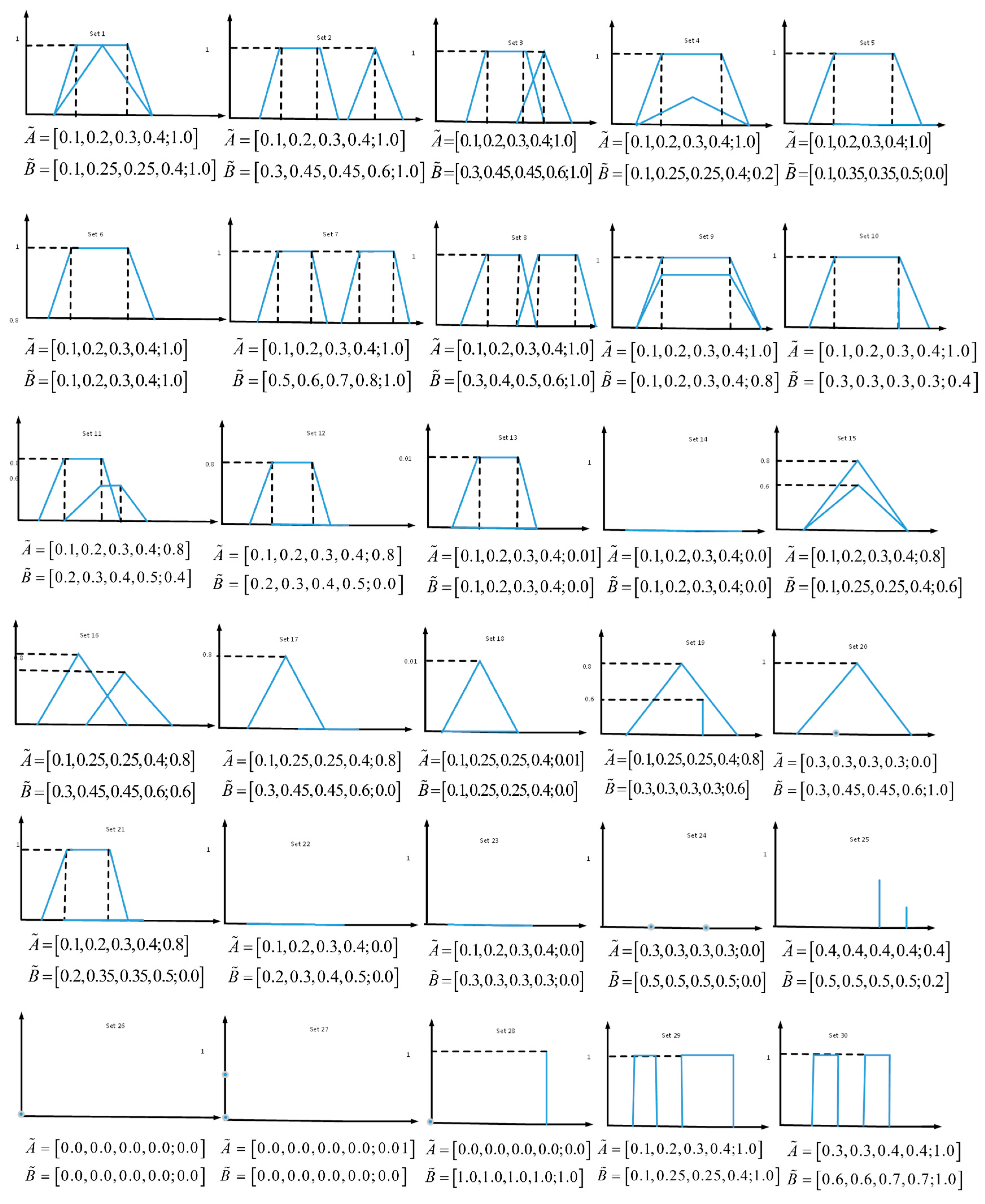
• From sets 9, 13, 15, 18, and 27 of Figure 2 and Table 1, we can see that the graphical representations of these sets were different, but looking at the calculation results of the method of Reference [35], the degree of similarity between $\tilde{A}$ and $\tilde{B}$ were equal to 1. However, from the results of Table 1, the degree of our proposed similarity was not equal to 1. This is in line with our intuition. Therefore, this proves that our method is better than that found in Reference [35].
• From sets 22 and 23 of Figure 2 and Table 1, as shown in Figure 2, the height and area of these geometric figures were equal to 0, but their perimeters are different. This means that the two type-2 fuzzy numbers were different. However, from Reference [38], the results from Table 1 were equal. Furthermore, our proposed similarity measure gives different results for these two type-2 fuzzy sets. This is more in line with human intuition. Hence, this shows that our method is superior to the method of Reference [38].
• From sets 24 and 26 of Figure 2 and Table 1, we can see that $\stackrel{\approx }{A}$ and $\stackrel{\approx }{B}$ have the same shape, perimeter, and height. However, according to the methods of References [30,32,36,37], it is difficult to obtain the similarity between $\stackrel{\approx }{A}$ and $\stackrel{\approx }{B}$ and unreasonable results are obtained. Moreover, from set 27, according to the results of the method of References [30,37], we find that the similarity was equal to 0. However, the similarity of geometrical figures was almost equal. Instead, the similarity of our methods was equal to 0.9928. This proves that our proposed similarity measure is more reasonable.
• From set 28 of Figure 2 and Table 1, we know that $\stackrel{\approx }{A}$ and $\stackrel{\approx }{B}$ were two completely different type-2 fuzzy numbers. Therefore, the similarity of our proposed method was equal to 0. However, from the calculation results of Reference [36], the results were unreasonable. Hence, our method is superior that found in Reference [36].
• From sets 29 and 30 of Figure 2 and Table 1, according to Reference [39], we can see that the result of the similarity measure of $\stackrel{\approx }{A}$ and $\stackrel{\approx }{B}$ were the same, but their graphical representation shows that they were different. In contrast, the results of the similarity of our methods were different. Therefore, our proposed method shows better performance.

In summary, the experimental results more clearly illustrate the advantages of the proposed similarity over other existing similarity measures. Its result is more intuitive and reasonable.

4. An Interval Type-2 Fuzzy Similarity-Based MABAC Approach in MCDM

Pamučar and Ćirović [41] originally introduced a new MCDM method, called multi-attributive border approximation area comparison (MABAC) method. Because of its directness and stability, this method becomes a practical decision tool. In this section, we present a modified MABAC based on similarity for handling MCDM problems under an interval type-2 fuzzy environment. The detailed process of the proposed method can be shown in Figure 3. Assume that X, is a set of alternatives and C is a set of attributes, where $X=\{x_1,x_2,\dots ,x_n\}$ and $C=\{c_1,c_2,\dots c_m\}$. Suppose the attribute weights are completely determined using DMs; that is, the weight vector $W={(w_j)}_{1\times m}$ of the attribute $c_j(j=1,2,\dots ,m)$ can be obtained in advance, where $w_j$ is an IT2FN. Let $R={(r_{ij})}_{n\times m}$ be an interval type-2 fuzzy decision matrix, where $r_{ij}$ is a linguistic term for the alternative $x_i$ with respect to the attribute $c_j$. Then, we can transform linguistic values into IT2FNs based on the corresponding rules in the

Table 2. Linguistic variables and their corresponding IT2FNs.

Importance	Rating	Corresponding IT2FNs
Absolutely low (AL)	Absolutely poor (AP)	[(0.0,0.0,0.0,0.0;1.0),(0.0,0.0,0.0,0.0;1.0)]
Very low (VL)	Very poor (VP)	[(0.0075,0.0075,0.015,0.0525;0.8),(0.0,0.0,0.02,0.07;1.0)]
Low (L)	Poor (P)	[(0.0875,0.12,0.16,0.1825;0.8),(0.04,0.10,0.18,0.23;1.0)]
Medium low (ML)	Medium poor (MP)	[(0.2325,0.255,0.325,0.3575;0.8),(0.17,0.22,0.36,0.42;1.0)]
Medium (M)	Fair (F)	[(0.4025,0.4525,0.5375,0.5675;0.8),(0.32,0.41,0.58,0.65;1.0)]
Medium high (MH)	Medium good (MG)	[(0.65,0.6725,0.7575,0.79;0.8),(0.58,0.63,0.80,0.86;1.0)]
High (H)	Good (G)	[(0.7825,0.815,0.885,0.9075;0.8),(0.72,0.78,0.92,0.97;1.0)]
Very high (VH)	Very good (VG)	[(0.9475,0.985,0.9925,0.9925;0.8),(0.93,0.98,1.0,1.0;1.0)]
Absolutely high (AH)	Absolutely good (AG)	[(1.0,1.0,1.0,1.0;1.0),(1.0,1.0,1.0,1.0;1.0)]

. In order to solve the aforementioned MCDM problems, a similarity-based MABAC method can be proposed consisting of the follow steps.

Step 1. Determine the alternatives and attributes, and construct the linguistic decision matrix $R={(r_{ij})}_{n\times m}(i=1,\dots ,n;j=1,\dots m)$, shown as follows:

$$R=\left[\begin{array}{cccc}{r}_{11}& r_{12}& \dots & r_{1m}\\ r_{21}& r_{22}& \dots & r_{2m}\\ ⋮& ⋮& \ddots & ⋮\\ r_{n1}& r_{n2}& \dots & r_{nm}\end{array}\right].$$

Based on Table 2, the linguistic value is converted to IT2FNs. This paper transforms the linguistic decision matrix $R={\left(r_{ij}\right)}_{n\times m}$ into the interval type-2 fuzzy decision matrix $T={\left(\stackrel{\approx }{t_{ij}}\right)}_{n\times m}$:

$$T=\left[\begin{array}{cccc}{\stackrel{\approx }{t}}_{11}& {\stackrel{\approx }{t}}_{12}& \dots & {\stackrel{\approx }{t}}_{1m}\\ {\stackrel{\approx }{t}}_{21}& {\stackrel{\approx }{t}}_{22}& \dots & {\stackrel{\approx }{t}}_{2m}\\ ⋮& ⋮& \ddots & ⋮\\ {\stackrel{\approx }{t}}_{n1}& {\stackrel{\approx }{t}}_{n2}& \dots & {\stackrel{\approx }{t}}_{nm}\end{array}\right].$$

Step 2. Normalize the interval type-2 decision matrix $T={\left(\stackrel{\approx }{t_{ij}}\right)}_{n\times m}$ into $N={\left({\stackrel{\approx }{n}}_{ij}\right)}_{n\times m}$. The normalization procedure is calculated as follows. For each attribute, $\stackrel{\approx }{r_{j+}^U}=\underset{1\le i\le m}{\max }\left(t_{ij4}^U\right)$ and $\stackrel{\approx }{r_{j-}^U}=\underset{1\le i\le m}{\min }\left(t_{ij1}^U\right),j=1,2,..,m$.

If $C_j$ is a benefit attribute, the normalization operation is as follows:

$${\stackrel{\approx }{n}}_{ij}=\left[\left(\frac{\stackrel{\approx }{r_{ij1}^L}-\stackrel{\approx }{r_{j-}^U}}{\stackrel{\approx }{r_{j+}^U}-\stackrel{\approx }{r_{j-}^U}},\frac{\stackrel{\approx }{r_{ij2}^L}-\stackrel{\approx }{r_{j-}^U}}{\stackrel{\approx }{r_{j+}^U}-\stackrel{\approx }{r_{j-}^U}},\frac{\stackrel{\approx }{r_{ij3}^L}-\stackrel{\approx }{r_{j-}^U}}{\stackrel{\approx }{r_{j+}^U}-\stackrel{\approx }{r_{j-}^U}},\frac{\stackrel{\approx }{r_{ij4}^L}-\stackrel{\approx }{r_{j-}^U}}{\stackrel{\approx }{r_{j+}^U}-\stackrel{\approx }{r_{j-}^U}};w_{R_{ij}}^L\right),\left(\frac{\stackrel{\approx }{r_{ij1}^U}-\stackrel{\approx }{r_{j-}^U}}{\stackrel{\approx }{r_{j+}^U}-\stackrel{\approx }{r_{j-}^U}},\frac{\stackrel{\approx }{r_{ij2}^U}-\stackrel{\approx }{r_{j-}^U}}{\stackrel{\approx }{r_{j+}^U}-\stackrel{\approx }{r_{j-}^U}},\frac{\stackrel{\approx }{r_{ij3}^U}-\stackrel{\approx }{r_{j-}^U}}{\stackrel{\approx }{r_{j+}^U}-\stackrel{\approx }{r_{j-}^U}},\frac{\stackrel{\approx }{r_{ij4}^U}-\stackrel{\approx }{r_{j-}^U}}{\stackrel{\approx }{r_{j+}^U}-\stackrel{\approx }{r_{j-}^U}};w_{R_{ij}}^U\right)\right].$$

(6)

If $C_j$ is a cost attribute, the normalization operation is as follows:

$${\stackrel{\approx }{n}}_{ij}=\left[\left(\frac{\stackrel{\approx }{r_{j+}^U}-\stackrel{\approx }{r_{ij4}^L}}{\stackrel{\approx }{r_{j+}^U}-\stackrel{\approx }{r_{j-}^U}},\frac{\stackrel{\approx }{r_{j+}^U}-\stackrel{\approx }{r_{ij3}^L}}{\stackrel{\approx }{r_{j+}^U}-\stackrel{\approx }{r_{j-}^U}},\frac{\stackrel{\approx }{r_{j+}^U}-\stackrel{\approx }{r_{ij2}^L}}{\stackrel{\approx }{r_{j+}^U}-\stackrel{\approx }{r_{j-}^U}},\frac{\stackrel{\approx }{r_{j+}^U}-\stackrel{\approx }{r_{ij1}^L}}{\stackrel{\approx }{r_{j+}^U}-\stackrel{\approx }{r_{j-}^U}};w_{R_{ij}}^L\right),\left(\frac{\stackrel{\approx }{r_{j+}^U}-\stackrel{\approx }{r_{ij4}^U}}{\stackrel{\approx }{r_{j+}^U}-\stackrel{\approx }{r_{j-}^U}},\frac{\stackrel{\approx }{r_{j+}^U}-\stackrel{\approx }{r_{ij3}^U}}{\stackrel{\approx }{r_{j+}^U}-\stackrel{\approx }{r_{j-}^U}},\frac{\stackrel{\approx }{r_{j+}^U}-\stackrel{\approx }{r_{ij2}^U}}{\stackrel{\approx }{r_{j+}^U}-\stackrel{\approx }{r_{j-}^U}},\frac{\stackrel{\approx }{r_{j+}^U}-\stackrel{\approx }{r_{ij1}^U}}{\stackrel{\approx }{r_{j+}^U}-\stackrel{\approx }{r_{j-}^U}};w_{R_{ij}}^U\right)\right].$$

(7)

Step 3. Determine the weight value $\stackrel{\approx }{w_{ij}}$ of the criterion $C_j$ and calculate the weight matrix. Compute the weighted matrix $V={\left(\stackrel{\approx }{v_{ij}}\right)}_{n\times m}$, where $\stackrel{\approx }{v_{ij}}=\stackrel{\approx }{w_{ij}}\times \stackrel{\approx }{n_{ij}}$.

Step 4. Calculate the border approximation area (BAA) matrix $G={\left({\stackrel{\approx }{g}}_j\right)}_{1\times m}$, where the border approximation area for each criterion is obtained according to Equation (1):

$$[(\frac{1}{p+q}{\left({\displaystyle \prod _{\begin{array}{l}i,j=1\\ i\ne j\end{array}}^n\left(p{v}_{i1}^L+q{v}_{j1}^L\right)}\right)}^{1/n(n-1)},\frac{1}{p+q}{\left({\displaystyle \prod _{\begin{array}{l}i,j=1\\ i\ne j\end{array}}^n\left(p{v}_{i2}^L+q{v}_{j2}^L\right)}\right)}^{1/n(n-1)},$$

$$\begin{gathered} \frac{1}{p+q}{\left({\displaystyle \prod _{\begin{array}{l}i,j=1\\ i\ne j\end{array}}^n\left(p{v}_{i3}^L+q{v}_{j3}^L\right)}\right)}^{1/n(n-1)},\frac{1}{p+q}{\left({\displaystyle \prod _{\begin{array}{l}i,j=1\\ i\ne j\end{array}}^n\left(p{v}_{i4}^L+q{v}_{j4}^L\right)}\right)}^{1/n(n-1)};\underset{i=1,2,\dots n}{\min }\left\{w_i^L\right\}), \\ (\frac{1}{p+q}{\left({\displaystyle \prod _{\begin{array}{l}i,j=1\\ i\ne j\end{array}}^n\left(p{v}_{i1}^U+q{v}_{j1}^U\right)}\right)}^{1/n(n-1)},\frac{1}{p+q}{\left({\displaystyle \prod _{\begin{array}{l}i,j=1\\ i\ne j\end{array}}^n\left(p{v}_{i2}^U+q{v}_{j2}^U\right)}\right)}^{1/n(n-1)}, \end{gathered}$$

$$\frac{1}{p+q}{\left({\displaystyle \prod _{\begin{array}{l}i,j=1\\ i\ne j\end{array}}^n\left(p{v}_{i3}^U+q{v}_{j3}^U\right)}\right)}^{1/n(n-1)},\frac{1}{p+q}{\left({\displaystyle \prod _{\begin{array}{l}i,j=1\\ i\ne j\end{array}}^n\left(p{v}_{i4}^U+q{v}_{j4}^U\right)}\right)}^{1/n(n-1)};\underset{i=1,2,\dots n}{\min }\left\{w_i^U\right\})].$$

(8)

Step 5. Compute of distance matrix $D={(\stackrel{}{d_{ij}})}_{n\times m}$ and $Q={(\stackrel{}{q_{ij}})}_{n\times m}$, where the element of the distance matrix is calculated as follows:

$$d_{ij}=1-s(\stackrel{\approx }{v_{ij}},\stackrel{\approx }{V_j^{}}),$$

(9)

$$q_{ij}=1-s(\stackrel{\approx }{g_j},\stackrel{\approx }{V_j^{}}),$$

(10)

where:

If $C_j$ is a benefit attribute, then we can define the ideal solution as follows:

$${\stackrel{\approx }{V}}_j^{}=\left[\left(v_{j1}^{L+},v_{j2}^{L+},v_{j3}^{L+},v_{j4}^{L+};w_j^{L+}\right),\left(v_{j1}^{U+},v_{j2}^{U+},v_{j3}^{U+},v_{j4}^{U+};w_j^{U+}\right)\right]$$

$$=[\left(\underset{i}{\max }(v_{ij}^L),\underset{i}{\max }(v_{ij}^L),\underset{i}{\max }(v_{ij}^L),\underset{i}{\max }(v_{ij}^L);\underset{i}{\max }(w_{ij}^L)\right),$$

$$\left(\underset{i}{\max }(v_{ij}^U),\underset{i}{\max }(v_{ij}^U),\underset{i}{\max }(v_{ij}^U),\underset{i}{\max }(v_{ij}^U);\underset{i}{\max }(w_{ij}^U)\right)].$$

(11)

If $C_j$ is a cost attribute, then we can define the ideal solution as follows:

$${\stackrel{\approx }{V}}_j^{}=\left[\left(v_{j1}^{L-},v_{j2}^{L-},v_{j3}^{L-},v_{j4}^{L-};w_j^{L-}\right),\left(v_{j1}^{U-},v_{j2}^{U-},v_{j3}^{U-},v_{j4}^{U-};w_j^{U-}\right)\right]$$

$$=[\left(\underset{i}{\min }(v_{ij}^L),\underset{i}{\min }(v_{ij}^L),\underset{i}{\min }(v_{ij}^L),\underset{i}{\min }(v_{ij}^L);\underset{i}{\min }(w_{ij}^L)\right),$$

$$\left(\underset{i}{\min }(v_{ij}^U),\underset{i}{\min }(v_{ij}^U),\underset{i}{\min }(v_{ij}^U),\underset{i}{\min }(v_{ij}^U);\underset{i}{\min }(w_{ij}^U)\right)].$$

(12)

$s\left(\stackrel{\approx }{v_{ij}},\stackrel{\approx }{V_j}\right)$ denotes that the similarity between the weighted matrix $V$ and the ideal solution $\stackrel{\approx }{V_j^{}}$ using Equation (3). $s\left(\stackrel{\approx }{g_j},\stackrel{\approx }{V_j}\right)$ denotes that the similarity between the matrix $G$ and the ideal solution using Equation (3). Then, we can obtain the distance matrix $M={(m_{ij})}_{n\times m}$, where:

$$m_{ij}=q_{ij}-d_{ij}.$$

(13)

Step 6. Obtain the ranking orders.

According to the principle of the MABAC method, we can know that if $m_{ij}=0$, the alternative $x_i$ could belongs to the border approximation area ($G$); if $m_{ij}>0$, the alternative $x_i$ belongs to the upper approximation area ($G^{+}$); and if $m_{ij}<0$, the alternative $x_i$ belongs to the lower approximation area ($G^{-}$):

$$x_i\in \{\begin{array}{l}{G}^{+}{,\mathrm{m}}_{\mathrm{ij}}>0,\\ G,{\mathrm{m}}_{\mathrm{ij}}=0,\\ G^{-}{,\mathrm{m}}_{\mathrm{ij}}<0.\end{array}$$

Since the ideal alternative $x_i^{+}$ is located on the upper approximation area ($G^{+}$), whereas the anti-ideal alternative $x_i^{-}$ is located on the lower approximation area ($G^{-}$) (see Figure 4), in order to select the best alternative, the criterion of the alternative is required as much as possible in the upper approximation area ($G^{+}$). Furthermore, by computing the final score value $S_i$, we can rank all the alternatives according to the decreasing value of $S_i$:

$$S(x_i)={\displaystyle \sum _{j=1}^m{m}_{ij}},(i=1,2,\dots n;j=1,2,\dots m).$$

(14)

5. Application in Selecting Medical Treatment

In this section, a patient-centered medical treatment selection problem was used to illustrate the effective application of the approach proposed in Section 4. In order to fully demonstrate the flexibility of the proposed similarity-based MABAC, we compared them with the other methods on the same medical data. The medical treatment selection problem is described as follows.

5.1. Problem Description

The case comes from the Department of Endocrinology, XiangYa Third Hospital in China. The patient was a 38-year-old female who was diagnosed with type-2 diabetes mellitus disease. Type-2 diabetes mellitus is known as adult-onset diabetes, occurring after 35 to 40 years old, accounting for more than 90% of diabetic patients. The disease can cause life-threatening complications, such as retinopathy, lower extremity ulcers, heart disease, and so on. The most typical symptoms of this disease are polydipsia, polyuria, bulimia, weight loss, and so on. In the early stage, the insulin function of patients with type-2 diabetes is not completely lost, so the treatment of this period is critical. If not actively treated, the ability of insulin B cells to secretion insulin will be completely lost, and diabetes complications will follow, and the patient's organs will suffer serious damage.

Based on the patient’s medical history and current physical condition, the attending doctor provided three treatment options, including insulin injection therapy (A₁), stem cell transplant therapy (A₂), and gastric bypass surgery (A₃). In order to facilitate the patients and their families with understanding the related knowledge for each treatment, the physician provided descriptions of the treatment options based on several evaluative criteria, including survival rate (C1), severity of the side effects (C2), severity of the complications (C3), probability of a cure (C4), discomfort index of the treatment (C5), cost (C6), number of days of hospitalization (C7), probability of a recurrence (C8), and self-care capacity (C9). Moreover, the specific description of the three treatment methods is summarized in

Table 3. Descriptions of the treatment methods.

Insulin injection therapy (A1)

(1) A very high survival rate

(2) The possibility of a reactive hypoglycemia

(3) The possibility of an allergic shock as a complication

(4) About a 40% probability of a cure

(5) No pain/discomfort during treatment

(6) Health insurance covers most of the expenses, with a low out-of-pocket expense

(7) Do not need hospitalization

(8) A significantly high probability of a recurrence

(9) A good prognosis for the patient’s self-care ability

Stem cell transplant therapy (A2)

(1) A high survival rate

(2) There are no obvious side effects

(3) The low possibility of diabetic nephropathy and retinopathy

(4) A very high probability of a cure

(5) There is some pain/discomfort during treatment

(6) Health insurance covers some of the expenses, with a moderately higher out-of-pocket expense

(7) A moderate hospitalization

(8) A low probability of a recurrence

(9) A moderate prognosis for the patient’s self-care capacity

Gastric bypass surgery (A3)

(1) A high survival rate

(2) The possibility of a stomach paralysis

(3) The possibility of a ketoacidosis or hypertonic coma

(4) A high probability of a cure

(5) There is some pain/discomfort during treatment

(6) Low coverage by the patient’s health insurance and very high out-of-pocket expenses

(7) A slightly shorter hospitalization than A2

(8) A low probability of a recurrence

(9) A moderate prognosis for the patient’s self-care capacity

. Taking into account the patient-centered principle, the doctor wanted the patient and her family members to participate in the discussion and assessment of treatment options. The assessment results are shown in

Table 4. The criterion importance weights and therapeutic ratings.

Criteria	Importance Weights	Treatment Options
		A1	A2	A3
C1 (survival rate)	AH	VG	G	G
C2 (severity of the side effects)	L	F	G	F
C3 (severity of the complications)	ML	P	MG	P
C4 (probability of a cure)	AH	MP	VG	G
C5 (discomfort index of the treatment)	VL	VG	P	P
C6 (cost)	M	G	MP	AP
C7 (number of days of hospitalization)	VH	AG	MP	F
C8 (probability of a recurrence)	H	AP	G	G
C9 (self-care capacity)	MH	G	F	F

.

5.2. Illustration of the Modified MABAC Approach

The interval type-2 similarity-based MABAC approach, proposed in Section 4, can be applied to solve the medical treatment selection problems.

Step 1. Translate linguistic terms into IT2FNs according to the nine-point linguistic rating scale introduced in Reference [51], which is shown in Table 2. According to Table 3, we can convert the evaluation term into IT2FNs. Then, we can construct a decision matrix $X={\left({\stackrel{\approx }{x}}_{ij}\right)}_{3\times 9}.$

$$X={\left[\begin{array}{ccc}\begin{array}{l}\left[\right(0.9475,0.985,0.9925,0.9925;0.8),\\ (0.93,0.98,1.0,1.0;1.0\left)\right]\end{array}& \begin{array}{l}\left[\right(0.7825,0.815,0.885,0.9075;0.8),\\ (0.72,0.78,0.92,0.97;1.0\left)\right]\end{array}& \begin{array}{l}\left[\right(0.7825,0.815,0.885,0.9075;0.8),\\ (0.72,0.78,0.92,0.97;1.0\left)\right]\end{array}\\ \begin{array}{l}\left[\right(0.4025,0.4525,0.5375,0.5675;0.8),\\ (0.32,0.41,0.58,0.65;1.0\left)\right]\end{array}& \begin{array}{l}\left[\right(0.7825,0.815,0.885,0.9075;0.8),\\ (0.72,0.78,0.92,0.97;1.0\left)\right]\end{array}& \begin{array}{l}\left[\right(0.4025,0.4525,0.5375,0.5675;0.8),\\ (0.32,0.41,0.58,0.65;1.0\left)\right]\end{array}\\ \begin{array}{l}\left[\right(0.0875,0.12,0.16,0.1825;0.8),\\ (0.04,0.10,0.18,0.23;1.0\left)\right]\end{array}& \begin{array}{l}\left[\right(0.65,0.6725,0.7575,0.79;0.8),\\ (0.58,0.63,0.80,0.86;1.0\left)\right]\end{array}& \begin{array}{l}\left[\right(0.0875,0.12,0.16,0.1825;0.8),\\ (0.04,0.10,0.18,0.23;1.0\left)\right]\end{array}\\ \begin{array}{l}\left[\right(0.2325,0.255,0.325,0.3575;0.8),\\ (0.17,0.22,0.36,0.42;1.0\left)\right]\end{array}& \begin{array}{l}\left[\right(0.9475,0.985,0.9925,0.9925;0.8),\\ (0.93,0.98,1.0,1.0;1.0\left)\right]\end{array}& \begin{array}{l}\left[\right(0.7825,0.815,0.885,0.9075;0.8),\\ (0.72,0.78,0.92,0.97;1.0\left)\right]\end{array}\\ \begin{array}{l}\left[\right(0.9475,0.985,0.9925,0.9925;0.8),\\ (0.93,0.98,1.0,1.0;1.0\left)\right]\end{array}& \begin{array}{l}\left[\right(0.0875,0.12,0.16,0.1825;0.8),\\ (0.04,0.10,0.18,0.23;1.0\left)\right]\end{array}& \begin{array}{l}\left[\right(0.0875,0.12,0.16,0.1825;0.8),\\ (0.04,0.10,0.18,0.23;1.0\left)\right]\end{array}\\ \begin{array}{l}\left[\right(0.7825,0.815,0.885,0.9075;0.8),\\ (0.72,0.78,0.92,0.97;1.0\left)\right]\end{array}& \begin{array}{l}\left[\right(0.2325,0.255,0.325,0.3575;0.8),\\ (0.17,0.22,0.36,0.42;1.0\left)\right]\end{array}& \begin{array}{l}\left[\right(0.0,0.0,0.0,0.0;1.0),\\ (0.0,0.0,0.0,0.0;1.0\left)\right]\end{array}\\ \begin{array}{l}\left[\right(1.0,1.0,1.0,1.0;1.0),\\ (1.0,1.0,1.0,1.0;1.0\left)\right]\end{array}& \begin{array}{l}\left[\right(0.2325,0.255,0.325,0.3575;0.8),\\ (0.17,0.22,0.36,0.42;1.0\left)\right]\end{array}& \begin{array}{l}\left[\right(0.4025,0.4525,0.5375,0.5675;0.8),\\ (0.32,0.41,0.58,0.65;1.0\left)\right]\end{array}\\ \begin{array}{l}\left[\right(0.0,0.0,0.0,0.0;1.0),\\ (0.0,0.0,0.0,0.0;1.0\left)\right]\end{array}& \begin{array}{l}\left[\right(0.7825,0.815,0.885,0.9075;0.8),\\ (0.72,0.78,0.92,0.97;1.0\left)\right]\end{array}& \begin{array}{l}\left[\right(0.7825,0.815,0.885,0.9075;0.8),\\ (0.72,0.78,0.92,0.97;1.0\left)\right]\end{array}\\ \begin{array}{l}\left[\right(0.7825,0.815,0.885,0.9075;0.8),\\ (0.72,0.78,0.92,0.97;1.0\left)\right]\end{array}& \begin{array}{l}\left[\right(0.4025,0.4525,0.5375,0.5675;0.8),\\ (0.32,0.41,0.58,0.65;1.0\left)\right]\end{array}& \begin{array}{l}\left[\right(0.4025,0.4525,0.5375,0.5675;0.8),\\ (0.32,0.41,0.58,0.65;1.0\left)\right]\end{array}\end{array}\right]}^T$$

Step 2. Normalize the interval type-2 decision matrix $X={\left({\stackrel{\approx }{x}}_{ij}\right)}_{3\times 9}$ into $N={\left({\stackrel{\approx }{n}}_{ij}\right)}_{3\times 9}.$

In this case, $C_1$,${\mathrm{C}}_4$,${\mathrm{C}}_8$,${\mathrm{C}}_9$ are benefit attributes, and $C_2$,$C_3$,$C_5$,${\mathrm{C}}_6$,${\mathrm{C}}_7$ are cost attributes. The matrix $N={\left({\stackrel{\approx }{n}}_{ij}\right)}_{3\times 9}$ can be calculated according to Equations (6) and (7).

$$N={\left[\begin{array}{ccc}\begin{array}{l}\left[\right(0.8125,0.9464,0.9732,0.9732;0.8),\\ (0.75,0.9286,1.0,1.0;1.0\left)\right]\end{array}& \begin{array}{l}\left[\right(0.9475,0.985,0.9925,0.9925;0.8),\\ (0.93,0.98,1.0,1.0;1.0\left)\right]\end{array}& \begin{array}{l}\left[\right(0.9475,0.985,0.9925,0.9925;0.8),\\ (0.93,0.98,1.0,1.0;1.0\left)\right]\end{array}\\ \begin{array}{l}\left[\right(0.6192,0.6654,0.7962,0.8731;0.8),\\ (0.4923,0.6,0.8615,1.0;1.0\left)\right]\end{array}& \begin{array}{l}\left[\right(0.4325,0.4625,0.5475,0.5975;0.8),\\ (0.35,0.42,0.59,0.68;1.0\left)\right]\end{array}& \begin{array}{l}[(0.21,0.2425,0.3275,0.35;0.8),\\ (0.14,0.2,0.37,0.42;1.0)]\end{array}\\ \begin{array}{l}[(0.8262,0.8537,0.9024,0.9421;0.8),\\ (0.7683,0.8293,0.9268,1.0;1.0)]\end{array}& \begin{array}{l}[(0.21,0.2425,0.3275,0.35;0.8),\\ (0.14,0.2,0.37,0.42;1.0)]\end{array}& \begin{array}{l}[(0.8175,0.84,0.88,0.9125;0.8),\\ (0.77,0.82,0.90,0.96;1.0)]\end{array}\\ \begin{array}{l}\left[\right(0.0753,0.1024,0.1657,0.2259;0.8),\\ (0.0,0.0602,0.2289,0.3012;1.0\left)\right]\end{array}& \begin{array}{l}\left[\right(0.9475,0.985,0.9925,0.9925;0.8),\\ (0.93,0.98,1.0,1.0;1.0\left)\right]\end{array}& \begin{array}{l}\left[\right(0.7825,0.815,0.885,0.9075;0.8),\\ (0.72,0.78,0.92,0.97;1.0\left)\right]\end{array}\\ \begin{array}{l}[(0.0075,0.0075,0.015,0.0524;0.8),\\ (0,0,0.02,0.07;1.0)]\end{array}& \begin{array}{l}[(0.8175,0.84,0.88,0.9125;0.8),\\ (0.77,0.82,0.9,0.96;1.0)]\end{array}& \begin{array}{l}[(0.0075,0.0075,0.015,0.0525;0.8),\\ (0,0,0.02,0.07;1.0)]\end{array}\\ \begin{array}{l}[(0.0925,0.1150,0.1850,0.2175;0.8),\\ (0.03,0.08,0.22,0.28;1.0)]\end{array}& \begin{array}{l}[(0.6425,0.9675,0.745,0.7675;0.8),\\ (0.58,0.64,0.78,0.83;1.0)]\end{array}& \begin{array}{l}[(1,1,1,1;1.0),\\ (1,1,1,1;1.0)]\end{array}\\ \begin{array}{l}[(0.9475,0.9985,0.9925,0.9925;0.8),\\ (0.93,0.98,1,1;1.0)]\end{array}& \begin{array}{l}[(0.6425,0.9675,0.7450,0.7675;0.8),\\ (0.58,0.64,0.78,0.83;1.0)]\end{array}& \begin{array}{l}[(0.4325,0.4625,0.5475,0.5975;0.8),\\ (0.35,0.42,0.59,0.68;1.0)]\end{array}\\ \begin{array}{l}\left[\right(0.0,0.0,0.0,0.0;1.0),\\ (0.0,0.0,0.0,0.0;1.0\left)\right]\end{array}& \begin{array}{l}\left[\right(0.7825,0.815,0.885,0.9075;0.8),\\ (0.72,0.78,0.92,0.97;1.0\left)\right]\end{array}& \begin{array}{l}\left[\right(0.7825,0.815,0.885,0.9075;0.8),\\ (0.72,0.78,0.92,0.97;1.0\left)\right]\end{array}\\ \begin{array}{l}\left[\right(0.0875,0.12,0.16,0.1825;0.8),\\ (0.04,0.10,0.18,0.23;1.0\left)\right]\end{array}& \begin{array}{l}\left[\right(0.4025,0.4525,0.5375,0.5675;0.8),\\ (0.32,0.41,0.58,0.65;1.0\left)\right]\end{array}& \begin{array}{l}\left[\right(0.4025,0.4525,0.5375,0.5675;0.8),\\ (0.32,0.41,0.58,0.65;1.0\left)\right]\end{array}\end{array}\right]}^T$$

Step 3. Determine the weight value $\stackrel{\approx }{w_{ij}}$ of the criterion $C_j(j=1,2,\dots ,9)$ from Table 3, and compute the weighted matrix $V={\left(\stackrel{\approx }{v_{ij}}\right)}_{3\times 9}$.

$$V={\left[\begin{array}{ccc}\begin{array}{l}[(0.7825,0.815,0.885,0.9075;0.8),\\ (0.72,0.78,0.92,0.97;1.0)]\end{array}& \begin{array}{l}[(0.9475,0.985,0.9925,0.9925;0.8),\\ (0.93,0.98,1,1;1.0)]\end{array}& \begin{array}{l}[(0.9475,0.985,0.9925,0.9925;0.8),\\ (0.93,0.98,1,1;1.0)]\end{array}\\ \begin{array}{l}[(0.0081,0.0138,0.0286,0.3262;0.8),\\ (0.0012,0.0080,0.0396,0.0644;1.0)]\end{array}& \begin{array}{l}[(0.0378,0.0555,0.0876,0.109;0.8),\\ (0.0238,0.0440,0.1332,0.1764;1.0)]\end{array}& \begin{array}{l}[(0.0184,0.0291,0.0524,0.0639;0.8),\\ (0.0056,0.02,0.0666,0.0966;1.0)]\end{array}\\ \begin{array}{l}[(0.1901,0.2142,0.0286,0.3262;0.8),\\ (\mathrm{0.1309.0.1804},0.3240,0.4032;1.0)]\end{array}& \begin{array}{l}[(0.0488,0.0618,0.106,0.1251;0.8),\\ (0.0238,0.044,0.1332,0.1764；1.0)]\end{array}& \begin{array}{l}[(0.1901,0.2142,0.0286,0.3262;0.8),\\ (0.1309,0.1804,0.3240,0.4032;1.0)]\end{array}\\ \begin{array}{l}[(0.2325,0.2550,0.325,0.3575;0.8),\\ (0.17,0.22,0.36,0.42;1.0)]\end{array}& \begin{array}{l}[(0.9475,0.9850,0.9925,0.9925;0.8),\\ (0.93,0.98,1,1;1.0)]\end{array}& \begin{array}{l}[(0.7825,0.8150,0.8850,0.9075;0.8),\\ (0.72,0.78,0.92,0.97;1.0)]\end{array}\\ \begin{array}{l}[(0.0001,0.0001,0.0002,0.0028;0.8),\\ (0,0,0.0004,0.0049;1.0)]\end{array}& \begin{array}{l}[(0.0061,0.0063,0.0013,0.0479;0.8),\\ (0,0,0.0180,0.0672;1.0)]\end{array}& \begin{array}{l}[(0.0001,0.0001,0,0.0028;0.8),\\ (0,0,0.0004,0.0049;1.0)]\end{array}\\ \begin{array}{l}[(0.0372,0.0520,0.0994,0.1234;0.8),\\ (0.0096,0.0328,0.1276,0.1820;1.0)]\end{array}& \begin{array}{l}[(0.2586,0.4468,0.4004,0.4356;0.8),\\ (0.1856,0.2624,0.4524,0.5395;1.0)]\end{array}& \begin{array}{l}[(0.4025,0.4525,0.5375,0.5675;0.8),\\ (0.32,0.41,0.58,0.65;1.0)]\end{array}\\ \begin{array}{l}[(0.8978,0.9835,0.9851,0.9851;0.8),\\ (0.8649,0.9604,1,1;1.0)]\end{array}& \begin{array}{l}[(0.6088,0.99530,0.7394,0.7617;0.8),\\ (0.5394,0.6272,0.78,0.83;1.0)]\end{array}& \begin{array}{l}[(0.4098,0.4556,0.5434,0.5930;0.8),\\ (0.3255,0.4116,0.59,0.68;1.0)]\end{array}\\ \begin{array}{l}[(0,0,0,0;1.0),\\ (0,0,0,0;1.0)]\end{array}& \begin{array}{l}[(0.6123,0.6642,0.7832,0.8236;1.0),\\ (0.5184,0.6084,0.8464,0.9409;1.0)]\end{array}& \begin{array}{l}[(0.6123,0.6642,0.7832,0.8236;0.8),\\ (0.5184,0.6084,0.8464,0.9409;1.0)]\end{array}\\ \begin{array}{l}[(0.0569,0.0807,0.1212,0.1442;0.8),\\ (0.0232,0.063,0.144,0.1978;1.0)]\end{array}& \begin{array}{l}[(0.2616,0.3043,0.4072,0.4483;0.8),\\ (0.1856,0.2583,0.4640,0.5590;1.0)]\end{array}& \begin{array}{l}[(0.2616,0.3043,0.4072,0.4483;0.8),\\ (0.1856,0.2583,0.4640,0.5590;1.0)]\end{array}\end{array}\right]}^T$$

Step 4. Compute the border approximation area matrix $G={\left({\stackrel{\approx }{g}}_j\right)}_{1\times 9}$.

The border approximation area vector $G$ can be obtained according to Equation (8).

$$G={\left[\begin{array}{c}[(0.8890,0.9247,0.9553,0.9633;0.8),(0.8540,0.9082,0.9726,0.9899;1.0)]\\ [(0.0388,0.0547,0.0420,0.1122;0.8),(0.0130,0.0393,0.1109,0.1595;1.0)]\\ [(0.1208,0.1415,0.0205,0.2370;0.8),(0.0742,0.1127,0.2409,0.3061;1.0)]\\ [(0.5565,0.5894,0.3056,0.4846;0.8),(0.4846,0.5520,0.6919,0.7413;1.0)]\\ [(0.0004,0.0004,0,0.0072;0.8),(0,0,0.0014,0.0117;1.0)]\\ [(0.1570,0.2191,0.2776,0.3125;0.8),(0.0829,0.1522,0.3223,0.3996;1.0)]\\ [(0.6073,0.7530,0.7342,0.7634;0.8),(0.5335,0.6282,0.7721,0.8264;1.0)]\\ [(0,0,0,0;1.0),(0,0,0,0;1.0)]\\ [(0.1573,0.1955,0.2719,0.3071;0.8),(0.0928,0.1614,0.3141,0.3954;1.0)]\end{array}\right]}^T$$

Step 5. Calculation of the distance matrix $M={(m_{ij})}_{3\times 9}$.

The distance matrix can be obtained according to Equations (9)–(13).

$$M=\left[\begin{array}{ccccccccc}0.1002& 0.0372& -0.0768& 0.2419& -0.0058& -0.1580& 0.2541& 0& -0.1405\\ -0.0634& -0.037& 0.0906& -0.4064& 0.0299& 0.0891& -0.0126& 0.6779& 0.1274\\ -0.0634& 0.0145& -0.0768& -0.2428& -0.0042& 0.2209& -0.1814& 0.6779& 0.1274\end{array}\right]$$

Step 6. Rank all alternatives.

The final score value $S(A_i)$ for each alternative can be obtained using Equation (14).

$$\begin{array}{l}S(A_1)=-0.3527,\\ S(A_2)=1.3279,\\ S(A_3)=1.2091.\end{array}$$

Through the calculation result of the similarity-based MABAC, the medical treatment can be ranked according to $A_2\succ A_3\succ A_1$ where the best alternative is $A_2$.

5.3. Comparison Analysis and Discussion

In order to further verify the effectiveness of the proposed similarity-based MABAC approach in the interval type-2 fuzzy environment, a comparative study was conducted with other approaches on the same decision data from Section 5.

(1) In Reference [52], Wan and Wang proposed an extended VIseKriterijumska Optimizacija I Kompromisno Resenje (VIKOR) method for multiple criteria decision problem.

According to the following formula from Reference [52], under the same medical data conditions, the results are as follows:

$$Q_i=v\frac{\left(S_i-S^{-}\right)}{\left(S^{+}-S^{-}\right)}+\left(1-v\right)\frac{\left(R_i-R^{-}\right)}{\left(R_i-R^{-}\right)},\mathrm{i}=1,2,3,$$

where $S^{+}=\underset{i}{\max }{S}_i$, $S^{-}=\underset{i}{\min }{S}_i$, $R^{+}=\underset{i}{\max }{R}_i$ and $R^{-}=\underset{i}{\max }{R}_i$, where it was supposed that $v=0.5$.

Then $Q_1=0.243,{\mathrm{Q}}_2=0.095,{\mathrm{Q}}_3=0.165$.

The ranking relations were identified as $A_2\succ A_3\succ A_1$. The result is the same as our proposed approach.

(2) In Reference [53], an extended TOPSIS method in an interval type-2 fuzzy environment was proposed by Liu. If we apply this method to the same medical data, we get the following results as shown in

Table 5. The calculation results of ${\Delta }_{\mathrm{ij}}^{+}$.

	C1	C2	C3	C4	C5	C6	C7	C8	C9
A1	0.1778	0.0529	0	0.6465	0.0158	0.3658	0	0.6526	0.2317
A2	0	0.0073	0.1339	0	0	0.1069	0.2099	0	0
A3	0	0.0362	0	0.1178	0.0158	0	0.4122	0	0

and

Table 6. The calculation results of ${\Delta }_{\mathrm{ij}}^{-}$.

	C1	C2	C3	C4	C5	C6	C7	C8	C9
A1	0	0.0287	0.1339	0	0	0	0.4122	0	0
A2	0.1178	0.0604	0	0.6465	0.0158	0.2589	0.2023	0.6526	0.2317
A3	0.1778	0.0406	0.1339	0.5287	0.0002	0.3658	0	0.6526	0.2317

.

According to the method from Reference [53], we can obtain the final value of the alternatives as follows:

$$C_1=0.4374,C_2=0.5745,C_3=0.5717.$$

Therefore, the final ranking was $A_2\succ A_3\succ A_1$.

(3) In order to elaborate on the advantages of the proposed similarity-based MABAC, the traditional MABAC method proposed in Reference [41] was used to deal with the same medical data. We used the Euclidean distance criterion to calculate the distance between the weighted matrix and the border matrix. The distance matrix $M={(m_{ij})}_{3\times 9}$ is shown as follows:

$$M=\left[\begin{array}{ccccccccc}-0.0929& -0.0457& 0.0725& -0.3095& -0.0029& -0.1598& 0.2626& 0& -0.1388\\ 0.0513& 0.007& -0.0862& 0.4211& 0.0252& 0.1184& 0.0154& 0.7372& 0.1266\\ 0.0513& -0.0254& 0.0725& 0.2769& -0.0029& 0.2268& 0.2022& 0.7372& 0.1266\end{array}\right]$$

Then, we obtained the score of the alternatives as follows:

$$S(A_1)=-0.4144,S(A_2)=1.4161,S(A_3)=1.2609.$$

Hence, the final order was $A_2\succ A_3\succ A_1$.

(4) To further illustrate the advantages of the proposed method, we extended the interval-valued ELimination Et Choix Traduisant la REalité (ELECTRE) method [54,55] to the medical treatment selection problem under the interval type-2 fuzzy number. By applying it to the same medical data, the aggregated outranking matrix could be determined as follows:

$$G=\left[\begin{array}{ccc}-& 0& 0\\ 1& -& 0\\ 1& 0& -\end{array}\right].$$

According to the information of the matrix $G$, outranking relationships were given as $\left(A_2,A_3\right)\succ A_1$.

(5) In this paper, the proposed similarity measure was combined with MABAC method to improve the accuracy of medical decision-making. Therefore, in order to further verify the efficiency of the proposed similarity measure, the similarity measure proposed by Patra and Mondal [38] was combined with the MABAC method to make a comparative analysis of the ranking results. First, the comparative similarity measure was extended to the interval type-2 fuzzy environment. Let $\stackrel{\approx }{A}$ and $\stackrel{\approx }{B}$ be two interval type-2 fuzzy numbers. The extended similarity formula is expressed as follows:

$$ar\left({\tilde{\tilde{A}}}^L\right)=\frac{\left(a_4^L+a_3^L-a_2^L-a_1^L\right)\times w_{{\tilde{\tilde{A}}}^L}}{2},$$

(15)

$$ar\left({\tilde{\tilde{A}}}^U\right)=\frac{\left(a_4^U+a_3^U-a_2^U-a_1^U\right)\times w_{{\tilde{\tilde{A}}}^U}}{2},$$

(16)

$$ar\left({\tilde{\tilde{B}}}^L\right)=\frac{\left(b_4^L+b_3^L-b_2^L-b_1^L\right)\times w_{{\tilde{\tilde{B}}}^L}}{2},$$

(17)

$$ar\left({\tilde{\tilde{B}}}^U\right)=\frac{\left(b_4^U+b_3^U-b_2^U-b_1^U\right)\times w_{{\tilde{\tilde{B}}}^U}}{2},$$

(18)

$$\begin{gathered} S\left(\tilde{\tilde{A}},\tilde{\tilde{B}}\right)=\sqrt{S\left({\tilde{\tilde{A}}}^L,{\tilde{\tilde{B}}}^L\right)\times S\left({\tilde{\tilde{A}}}^U,{\tilde{\tilde{B}}}^U\right)}, \\ =\sqrt{\left(1-\frac{1}{4}{\displaystyle \sum _{i=1}^4\left|a_i^L-b_i^L\right|}\right)\times \left(1-\frac{1}{2}\left\{\left|ar\left({\tilde{\tilde{A}}}^L\right)-ar\left({\tilde{\tilde{B}}}^L\right)\right|+\left|w_{{\tilde{\tilde{A}}}^L}-w_{{\tilde{\tilde{B}}}^L}\right|\right\}\right)} \\ \times \sqrt{\left(1-\frac{1}{4}{\displaystyle \sum _{i=1}^4\left|a_i^U-b_i^U\right|}\right)\times \left(1-\frac{1}{2}\left\{\left|ar\left({\tilde{\tilde{A}}}^U\right)-ar\left({\tilde{\tilde{B}}}^U\right)\right|+\left|w_{{\tilde{\tilde{A}}}^U}-w_{{\tilde{\tilde{B}}}^U}\right|\right\}\right)}. \end{gathered}$$

(19)

Then, the same medical data is introduced into the similarity measure and the score of the alternatives is calculated as follows:

$$S(A_1)=-0.1144,S(A_2)=1.0161,S(A_3)=-0.2609.$$

Hence, the final order was $A_2\succ A_1\succ A_3$.

The results of all the methods are compared in

Table 7. Ranking results according to six methods.

Methods	Ranking Results	The Best Alternatives
The extended VIKOR method [52]	$A_2\succ A_3\succ A_1$	$A_2$
The extended TOPSIS method [53]	$A_2\succ A_3\succ A_1$	$A_2$
The traditional MABAC method [41]	$A_2\succ A_3\succ A_1$	$A_2$
The modified ELECTRE method [54]	$\left(A_2,A_3\right)\succ A_1$	$A_2,A_3$
The similarity-based MABAC method [38]	$A_2\succ A_1\succ A_3$	$A_2$
The proposed MABAC method	$A_2\succ A_3\succ A_1$	$A_2$

, $A_2$ was always the best alternative, and $A_1$ was always the worst alternative, except when using the last method. Moreover, we can know that the ranking order of the other five methods gave the same ranking result except for the ELECTRE method and the similarity-based MABAC method. From the ranking relationship of the ELECTRE method, we cannot determine the best treatment alternative. Therefore, the result shows that our proposed approaches were reasonable and effective. In addition, the ranking results of the similarity-based MABAC method showed that the proposed similarity combined with MABAC method had a higher decision accuracy.

Additionally, to prove the proposed MABAC method is superior to the other five methods in the application of type-2 diabetes mellitus medical care selection, the computational time in seconds was calculated, as shown in Figure 5. Among them, the modified ELECTRE method consumed the least amount of time. Although the proposed MABAC method did not consume the least time, it also proved its superiority in time complexity compared with the other four methods.

6. Conclusions

In this paper, the new algorithm of the patient-centered treatment selection problem was studied in detail in an interval type-2 fuzzy environment. The MABAC algorithm was extended to efficiently solve the patient-centered care problem. First, to overcome the limitations of the existing similarity measures, we proposed new similarity measures based on the geometric properties. Simultaneously, it proved to be in accordance with the proposed triangular inequality property, which was first presented in interval type-2 fuzzy environment. Next, a comparative experiment proved the superiority of the proposed similarity measure. Then, in order to optimize the composition of the MCDM method and improve the efficiency and accuracy of the calculation process, we presented a similarity-based MABAC approach to deal with the medical treatment selection problem in patient-centered environment. Finally, a type-2 diabetes treatment selection problem was given to illustrate the viability and flexibility of the proposed similarity-based MABAC method. Meanwhile, a comparison analysis was presented in Table 7 and Figure 5. For future research, we will explore other forms of interval type-2 fuzzy similarity under other background conditions. In addition, we can extend and explore other decision-making methods based on IT2FNs to improve the accuracy of medical care decision-making.

References

1. Redman, R.W. Patient-centered care: An unattainable ideal? Res. Theory Nurs. Pract. 2004, 18, 11. [Google Scholar] [CrossRef] [PubMed]
2. Hu, J.; Chen, D.; Liang, P. A Novel Interval Three-Way Concept Lattice Model with Its Application in Medical Diagnosis. Mathematics 2019, 7, 103. [Google Scholar] [CrossRef]
3. Pelzang, R. Time to learn: Understanding patient-centred care. Br. J. Nurs. 2010, 19, 912–917. [Google Scholar] [CrossRef] [PubMed]
4. Steiger, N.J.; Balog, A. Realizing patient-centered care: Putting patients in the center, not the middle. Front. Health Serv. Manag. 2010, 26, 15–25. [Google Scholar] [CrossRef]
5. Epstein, R.M. The science of patient-centered care. J. Fam. Pract. 2000, 49, 805–807. [Google Scholar] [PubMed]
6. Mccormack, B.; Mccance, T.V. Development of a framework for person-centred nursing. J. Adv. Nurs. 2006, 56, 472–479. [Google Scholar] [CrossRef]
7. Lutz, B.J.; Bowers, B.J. Patient-centered care: Understanding its interpretation and implementation in health care. Res. Theory Nurs. Pract. 2000, 14, 165–183; discussion 183–187. [Google Scholar]
8. Lee, Y.Y.; Lin, J.L. Do patient autonomy preferences matter? Linking patient-centered care to patient-physician relationships and health outcomes. Soc. Sci. Med. 2010, 71, 1811–1818. [Google Scholar] [CrossRef]
9. Edwards, M.; Davies, M.; Edwards, A. What are the external influences on information exchange and shared decision-making in healthcare consultations: A meta-synthesis of the literature. Patient Educ. Couns. 2009, 75, 37–52. [Google Scholar] [CrossRef]
10. Qin, J.; Liu, X. Multi-attribute group decision making using combined ranking value under interval type-2 fuzzy environment. Inf. Sci. 2015, 297, 293–315. [Google Scholar] [CrossRef]
11. Qin, J.; Liu, X.; Pedrycz, W. An extended VIKOR method based on prospect theory for multiple attribute decision making under interval type-2 fuzzy environment. Knowl. Based Syst. 2015, 86, 116–130. [Google Scholar] [CrossRef]
12. Wang, J.Q.; Peng, J.J.; Zhang, H.Y.; Chen, X.H. Outranking approach for multi-criteria decision-making problems with hesitant interval-valued fuzzy sets. Soft Comput. 2017. [Google Scholar] [CrossRef]
13. Zhang, X.Y.; Zhang, H.Y.; Wang, J.Q. Discussing incomplete 2-tuple fuzzy linguistic preference relations in multi-granular linguistic MCGDM with unknown weight information. Soft Comput. 2017, 20, 958–969. [Google Scholar] [CrossRef]
14. Peng, H.-G.; Wang, X.-K.; Wang, T.-L.; Wang, J.-Q. Multi-criteria game model based on the pairwise comparisons of strategies with Z-numbers. Appl. Soft Comput. 2019, 74, 451–465. [Google Scholar] [CrossRef]
15. Sun, R.; Hu, J.; Chen, X. Novel single-valued neutrosophic decision-making approaches based on prospect theory and their applications in physician selection. Soft Comput. 2019, 23, 211–225. [Google Scholar] [CrossRef]
16. Liang, P.; Hu, J.; Liu, Y.; Chen, X. Public resources allocation using an uncertain cooperative game among vulnerable groups. Kybernetes 2018. [Google Scholar] [CrossRef]
17. Yang, Y.; Hu, J.; Liu, Y.; Chen, X. Alternative selection of end-of-life vehicle management in China: A group decision-making approach based on picture hesitant fuzzy measurements. J. Clean. Prod. 2019, 206, 631–645. [Google Scholar] [CrossRef]
18. Zadeh, L.A. The Concept of a Linguistic Variable and its Application to Approximate Reasoning—I. Inf. Sci. 1974, 8, 199–249. [Google Scholar] [CrossRef]
19. Yang, Y.; Hu, J.; Liu, Y. Doctor recommendation based on an intuitionistic normal cloud model considering patient preferences. Cogn. Comput. 2018. [Google Scholar] [CrossRef]
20. Castillo, O.; Amador-Angulo, L.; Castro, J.R.; Garcia-Valdez, M. A comparative study of type-1 fuzzy logic systems, interval type-2 fuzzy logic systems and generalized type-2 fuzzy logic systems in control problems. Inf. Sci. 2016, 354, 257–274. [Google Scholar] [CrossRef]
21. Sanchez, M.A.; Castillo, O.; Castro, J.R. Generalized Type-2 Fuzzy Systems for controlling a mobile robot and a performance comparison with Interval Type-2 and Type-1 Fuzzy Systems. Expert Syst. Appl. 2015, 42, 5904–5914. [Google Scholar] [CrossRef]
22. Yang, Y.; Hu, J.; Sun, R.; Chen, X. Medical tourism estinations prioritization using group decision making method with neutrosophic fuzzy preference relations. Sci. Iran. Trans. E Ind. Eng. 2018, 25, 3744–3764. [Google Scholar]
23. Hu, J.; Zhang, X.; Yang, Y.; Liu, Y.; Chen, X. New doctors ranking system based on VIKOR method. Int. Trans. Oper. Res. 2018. [Google Scholar] [CrossRef]
24. Castillo, O.; Cervantes, L.; Soria, J.; Sanchez, M.; Castro, J.R. A Generalized Type-2 Fuzzy Granular Approach with Applications to Aerospace. Inf. Sci. Int. J. 2016, 354, 165–177. [Google Scholar] [CrossRef]
25. Ontiveros-Robles, E.; Melin, P.; Castillo, O. Comparative analysis of noise robustness of type 2 fuzzy logic controllers. Kybernetika 2018, 54, 175–201. [Google Scholar] [CrossRef]
26. Cervantes, L.; Castillo, O. Type-2 fuzzy logic aggregation of multiple fuzzy controllers for airplane flight control. Inf. Sci. 2015, 324, 247–256. [Google Scholar] [CrossRef]
27. Cazarez-Castro, N.R.; Aguilar, L.T.; Castillo, O. Designing Type-1 and Type-2 Fuzzy Logic Controllers via Fuzzy Lyapunov Synthesis for nonsmooth mechanical systems. Eng. Appl. Artif. Intell. 2012, 25, 971–979. [Google Scholar] [CrossRef]
28. Li, J.; Wang, J.Q.; Hu, J.H. Interval-valued n-person cooperative games with satisfactory degree constraints. Cent. Eur. J. Oper. Res. 2018. [Google Scholar] [CrossRef]
29. Ji, P.; Zhang, H.Y.; Wang, J.Q. A Fuzzy Decision Support Model With Sentiment Analysis for Items Comparison in e-Commerce: The Case Study of PConline.com. IEEE Trans. Syst. Man Cybern. Syst. 2018. [Google Scholar] [CrossRef]
30. Wei, S.H.; Chen, S.M. A new approach for fuzzy risk analysis based on similarity measures of generalized fuzzy numbers. Expert Syst. Appl. 2009, 36, 589–598. [Google Scholar] [CrossRef]
31. Chen, S.M.; Chen, J.H. A new method for ranking generalized fuzzy numbers for handling fuzzy risk analysis problems. In Proceedings of the Joint Conference on Information Sciences, JCIS 2006, Kaohsiung, Taiwan, 8–11 October 2006; pp. 1196–1199. [Google Scholar]
32. Chen, J.H.; Chen, S.M. A new method to measure the similarity between Interval-valued fuzzy numbers. In Proceedings of the International Conference on Machine Learning and Cybernetics, Hong Kong, China, 19–22 August 2007; pp. 1123–1126. [Google Scholar]
33. Wang, G.; Li, X. Correlation and information energy of interval-valued fuzzy numbers. Fuzzy Sets Syst. 1999, 103, 169–175. [Google Scholar] [CrossRef]
34. Sanchez, M.A.; Castillo, O.; Castro, J.R. Information granule formation via the concept of uncertainty-based information with Interval Type-2 Fuzzy Sets representation and Takagi–Sugeno–Kang consequents optimized with Cuckoo search. Appl. Soft Comput. 2015, 27, 602–609. [Google Scholar] [CrossRef]
35. Chen, S. New methods for subjective mental workload assessment and fuzzy risk analysis. Cybern. Syst. 1996, 27, 449–472. [Google Scholar] [CrossRef]
36. Chen, S.J.; Chen, S.M. A new method to measure the similarity between fuzzy numbers. In Proceedings of the 10th IEEE International Conference on Fuzzy Systems, Melbourne, Australia, 2–5 December 2001; pp. 208–214. [Google Scholar]
37. Hejazi, S.R.; Doostparast, A.; Hosseini, S.M. An improved fuzzy risk analysis based on a new similarity measures of generalized fuzzy numbers. Expert Syst. Appl. 2011, 38, 9179–9185. [Google Scholar] [CrossRef]
38. Patra, K.; Mondal, S.K. Fuzzy risk analysis using area and height based similarity measure on generalized trapezoidal fuzzy numbers and its application. Appl. Soft Comput. 2015, 28, 276–284. [Google Scholar] [CrossRef]
39. Cui, W.; Xu, Z. A method for fuzzy risk analysis based on the new similarity of trapezoidal fuzzy numbers. In Proceedings of the IEEE International Conference on Granular Computing, Nanchang, China, 17–19 August 2009; pp. 113–116. [Google Scholar]
40. Yang, Y.; Hu, J.; Liu, Y.; Chen, X. A multi-period hybrid decision support model for medical diagnosis and treatment based on similarities and three-way decision theory. Expert Syst. 2019. [Google Scholar] [CrossRef]
41. Pamucar, D.; Cirovic, G. The selection of transport and handling resources in logistics centers using multi-attributive border approximation area comparison (MABAC). Expert Syst. Appl. 2015, 42, 3016–3028. [Google Scholar] [CrossRef]
42. Sun, R.; Hu, J.; Zhou, J.; Chen, X. A hesitant fuzzy linguistic projection-based MABAC method for patients’ prioritization. Int. J. Fuzzy Syst. 2018, 20, 2144–2160. [Google Scholar] [CrossRef]
43. Xue, Y.X.; You, J.X.; Lai, X.D.; Liu, H.C. An interval-valued intuitionistic fuzzy MABAC approach for material selection with incomplete weight information. Appl. Soft Comput. 2016, 38, 703–713. [Google Scholar] [CrossRef]
44. Peng, X.; Yang, Y. Pythagorean fuzzy choquet integral based MABAC method for multiple attribute group decision making. Int. J. Intell. Syst. 2016, 31, 989–1020. [Google Scholar] [CrossRef]
45. Singh, N.; Tyagi, K. Ranking of services for reliability estimation of SOA system using fuzzy multicriteria analysis with similarity-based approach. Int. J. Syst. Assur. Eng. Manag. 2017, 8, 317–326. [Google Scholar] [CrossRef]
46. Hu, Y.C. Nonadditive similarity-based single-layer perceptron for multi-criteria collaborative filtering. Neurocomputing 2014, 129, 306–314. [Google Scholar] [CrossRef]
47. Greenfield, S.; Chiclana, F.; Coupland, S.; John, R. The Collapsing Method of Defuzzification for Discretised Interval Type-2 Fuzzy Sets. Inf. Sci. 2007, 179, 2055–2069. [Google Scholar] [CrossRef]
48. Chen, S.M.; Yang, M.W.; Lee, L.W.; Yang, S.W. Fuzzy multiple attributes group decision-making based on ranking interval type-2 fuzzy sets. Expert Syst. Appl. Int. J. 2017, 44, 1665–1673. [Google Scholar]
49. Chen, S.J.; Chen, S.M. Fuzzy risk analysis based on the ranking of generalized trapezoidal fuzzy numbers. Inf. Sci. 2007, 26, 1–11. [Google Scholar] [CrossRef]
50. Gong, Y.; Hu, N.; Zhang, J.; Liu, G.; Deng, J. Multi-attribute group decision making method based on geometric Bonferroni mean operator of trapezoidal interval type-2 fuzzy numbers. Comput. Ind. Eng. 2015, 81, 167–176. [Google Scholar] [CrossRef]
51. Chenabc, T.Y. The extended QUALIFLEX method for multiple criteria decision analysis based on interval type-2 fuzzy sets and applications to medical decision making. Eur. J. Oper. Res. 2013, 226, 615–625. [Google Scholar]
52. Wan, S.P.; Wang, Q.Y.; Dong, J.Y. The extended VIKOR method for multi-attribute group decision making with triangular intuitionistic fuzzy numbers. Knowl. Based Syst. 2013, 52, 65–77. [Google Scholar] [CrossRef]
53. Liu, P. An extended TOPSIS method for multiple attribute group decision making based on generalized interval-valued trapezoidal fuzzy numbers. J. Comput. Anal. Appl. 2011, 6, 766–776. [Google Scholar]
54. Vahdani, B.; Jabbari, A.H.K.; Roshanaei, V.; Zandieh, M. Extension of the ELECTRE method for decision-making problems with interval weights and data. Int. J. Adv. Manuf. Technol. 2010, 50, 793–800. [Google Scholar] [CrossRef]
55. Vahdani, B.; Hadipour, H. Extension of the ELECTRE method based on interval-valued fuzzy sets. Soft Comput. 2011, 15, 569–579. [Google Scholar] [CrossRef]
Figure 1. An interval type-2 fuzzy number A ˜ ˜ .
Mathematics 07 00140 g001
Figure 2. Graphical representation of 30 different sets of general type-2 fuzzy numbers (GT2FNs).
Mathematics 07 00140 g002
Figure 3. Flow diagram of the proposed approach. IT2FNs: interval type-2 fuzzy numbers, MABAC: multi-attributive border approximation area comparison.
Mathematics 07 00140 g003
Figure 4. Graphical presentation of G + , G , and G .
Mathematics 07 00140 g004
Figure 5. Comparison results in terms of CPU time.
Mathematics 07 00140 g005