Article

On Inverses of the Dirac Comb

by
Jens V. Fischer
1,2,* and
Rudolf L. Stens
2
1
German Aerospace Center (DLR), Microwaves and Radar Institute, 82234 Wessling, Germany
2
Lehrstuhl A für Mathematik, RWTH Aachen University, 52056 Aachen, Germany
*
Author to whom correspondence should be addressed.
Mathematics 2019, 7(12), 1196; https://doi.org/10.3390/math7121196
Submission received: 8 November 2019 / Revised: 30 November 2019 / Accepted: 2 December 2019 / Published: 6 December 2019

Abstract

:
We determine tempered distributions which convolved with a Dirac comb yield unity and tempered distributions, which multiplied with a Dirac comb, yield a Dirac delta. Solutions of these equations have numerous applications. They allow the reversal of discretizations and periodizations applied to tempered distributions. One of the difficulties is the fact that Dirac combs cannot be multiplied or convolved with arbitrary functions or distributions. We use a theorem of Laurent Schwartz to overcome this difficulty and variants of Lighthill’s unitary functions to solve these equations. The theorem we prove states that double-sided (time/frequency) smooth partitions of unity are required to neutralize discretizations and periodizations on tempered distributions.

Graphical Abstract

1. Introduction

The theory of generalized functions [1,2,3,4,5,6,7,8,9,10,11,12,13,14,15,16,17,18,19,20,21,22,23,24,25], an overview is given in Figure 1 (cf. Section 2.3), is known for its generality but also for its strictness not to allow arbitrary multiplication and arbitrary convolution among generalized functions [26,27,28,29,30,31,32,33,34] and, as a result of this, other theories have already been proposed to evade these difficulties. These difficulties are, however, not an inadequacy of the theory but rather consequences of a phenomenon known as the Heisenberg uncertainty principle. Laurent Schwartz’ theory of generalized functions effortlessly handles such difficulties.
It is also a setting that extends the idea of Fourier transformation and the only way today to rigorously treat Dirac delta functions [35] and Dirac combs [36] which turn out to be the derivatives of discontinuities in functions. All functions and generalized functions become infinitely differentiable in this way. This, in turn, is an indispensable tool in physics for solving differential equations [19,21,37,38,39]; hence, to describe natural laws. Laurent Schwartz’ theory is, furthermore, the first and only theory which explains Fourier series rigorously [5]. Fourier series allow us to write functions which cannot be derived continuously (e.g., the saw tooth [40]), as a superposition of infinitely differentiable functions (complex exponentials). In conventional calculus, this is a contradiction, and hence, “ ” is sometimes written instead of “=”. But there is indeed an equality between periodic functions and their Fourier series. It holds in the generalized functions sense. The theory of generalized functions is, therefore, also called the completion of functional analysis [5,24]. It is already the default setting in several branches of physics [41,42,43,44,45,46,47,48,49] and electrical engineering [40,50,51,52,53,54]. In a similar way as complex numbers complete the idea of numbers, generalized functions complete the idea of functions. An excellent overview of the many generalization methods unified within this theory (seven equivalent methods in order to generalize the ideas of “integration” and “differentiation”) and the many problems solved with it are given in Charts 1 and 2 in Lützen [55], pp. 222–223. For a brief introduction to distribution theory we recommend reading the introductory remarks in Halperin [3], Temple [4], Lighthill [5], Zemanian [12], Osgood [51] and Debnath [56], or the motivation sections in our previous studies [57,58,59].
The overall goal in this study is to introduce counter-operations which neutralize discretizations and periodizations, respectively. An interaction between discretization (sampling) and periodization (replicating) is sufficiently well-known. It can be found in Bracewell [60], Gasquet [40], or in Kammler [61] for example. However, it is not instantaneously clear that these operations can (residue-free) be reversed within the space of tempered distributions. A major barrier is the fact that tempered distributions cannot be multiplied or convolved with arbitrary other tempered distributions. To overcome this we use a theorem of Laurent Schwartz (Lemma 1) which states that convolution products exist if one of the two factors is (finitely) summable ( O C ), and equivalently, multiplication products exist if one of the two factors is (infinitely) differentiable ( O M ). It has, to the best of our knowledge, never been shown so far that discretizations and periodizations can be neutralized within the setting of generalized functions. The theorem presented below (Theorem 1) will be a foundation for generalized functions calculus because it interconnects four different forms of unity ( Ω , 1 , III , δ ).
We proceed as follows. Section 2 familiarizes the reader with the generalized functions terminology, Section 3 summarizes foundations laid in previous studies and Section 4 determines the convolution and multiplication inverses of the Dirac comb. This will serve us as a foundation for later studies. Our distant goal is it to extend the classical sampling theorem to the space of tempered distributions where it is known to fail most generally [40]. We briefly discuss this in Section 5.

2. Notation

All spaces of ordinary and generalized functions are denoted as in the standard literature [1,2,8,9,21]. The term “distribution” is used in the sense of Laurent Schwartz, where all functions and generalized functions are smooth (infinitely differentiable) and “ultradistributions”; the Fourier transform of “distributions”, are understood in the sense of Sebastião e Silva [62]; cf. Zemanian [8], Hoskins [20] and Walter [21]. The “unitary ordinary frequency” or “normalized” Fourier transform of conventional functions is
f ^ ( σ ) : = R n f ( t ) e 2 π i t · σ d t n = f , e 2 π i t · σ ,
where t · σ is the usual inner product in R n , and for generalized functions f S , it is F f , φ : = f , F φ for φ S . We denote them as F ( f ) or F f or simply f ^ . The expression f , φ f ( φ ) is the application of f to some test function φ . It naturally extends the usual inner product on Lebesgue-square integrable functions to the space of tempered distributions [23,63,64,65,66,67]. The expression f f , 1 denotes the integral of f in the tempered distributions sense [4,9] and the integral symbol f ( t ) d t is only used for ordinary Lebesgue integrable functions f ( t ) . The s i n c function is defined to be 1 at t = 0 and s i n c ( t ) : = s i n ( π t ) / ( π t ) otherwise, and r e c t : = F ( s i n c ) is its Fourier transform. It equals 1 within the interval 1 / 2 , + 1 / 2 , 1 / 2 at t = 1 / 2 and t = + 1 / 2 and zero otherwise [68,69]. We prefer using r e c t instead of the characteristic function of an interval χ which cannot take on values other than 0 or 1.

2.1. Equality between Generalized Functions

An equality f = g between two ordinary functions usually means that the equality f ( t ) = g ( t ) holds for all admissible t R n . In contrast to this, values f ( t ) and g ( t ) may not exist for tempered distributions f , g S . We therefore say that f = g “in the tempered distributions sense” if f ( φ ) = g ( φ ) holds for all admissible φ S ( R n ) . In other words, f applied to φ yields the same as g applied to φ for admissible φ . More generally, φ X is admissible for f X if f , φ < ; i.e., if f belongs to the topological dual of X. The classical comprehension of a function f arises whenever f ( φ ) approaches f ( t ) because φ tends to be the Dirac delta at t R n . Any test function argumentation is, moreover, avoided if symbolic calculation rules can be applied which are already known to be true; see the rules in [59] for example. The idea is to gather as many rules as possible to be able to calculate pure symbolically on (generalized) functions level instead of operating “pointwise”; i.e., on φ S ( R n ) in this case. A proof of the rules F 1 = δ and F δ = 1 can be found in Gasquet [40], for example.

2.2. Vector-Valued Generalized Functions

By denoting function spaces X and distribution spaces X , we actually mean X ( R n ) or X ( R n ) , respectively, where n 1 is an integer. For simplicity, we restrict ourselves to n = 1 in this study and for n > 1 ; i.e., for vector-valued functions and distributions, we would like to refer the reader to our previous studies [57,70]. One may, however, easily transfer these results to the general case by replacing the real number T by a vector T R n , and the condition T > 0 then means that T is greater than zero in all its components. The vector 1 / T in subscripts of operators then means that T is taken reciprocal in all of its components and T or 1 / T in front of operators is indeed a scalar but the product of all its components in T or 1 / T , respectively. This scalar in front of operators (see Tables 1–3 in [59]) arises due to the volume-preserving property of the Fourier transform (Corollary 1 in [57]). It can be traced back to elementary integration rules (e.g., Example 12.2 in [71]).

2.3. Spaces of Generalized Functions

The intersection of distributions D (in the sense of Schwartz [1,2,3,4,5,6,7,8,9,10,11,12,13,14,15,16,17,18,19,20,21,22,23,24,25]) and ultradistributions Z (in the sense of Sebastião e Silva [20,22,62,72,73]) which map onto each other via the Fourier transform, F ( D ) = Z and F ( Z ) = D , is the space of tempered distributions S = F ( S ) . It contains the space of multiplication operators O M (smooth slowly growing functions) and the space of convolution operators O C (rapidly deceasing tempered distributions), where F ( O M ) = O C and F ( O C ) = O M [18]. A particular case of these operators are Paley-Wiener functions P W (entire slowly growing functions [74]) and compactly supported tempered distributions E , where F ( P W ) = E and F ( E ) = P W . A space of functions which are both, convolution and multiplication operators, is the Schwartz space S = F ( S ) of smooth rapidly decreasing functions. It particularly contains (see, e.g., [8,21,22]), the space of smooth, time-limited functions D , and the space of smooth band-limited functions Z , where F ( D ) = Z and F ( Z ) = D .

2.4. Smooth Functions versus Generalized Functions

For the reader’s convenience, we summarize Laurent Schwartz’ diagram [2], p. 170, of continuously embedded spaces of (ordinarily smooth) functions and (in the generalized functions sense smooth) generalized functions in Figure 1. As an additional feature we also depict Fourier transform pairings (red versus blue) and their intersections (violet) in this figure. The left and the right-hand side are accordingly mirror-inverted Fourier transforms of one another. Special pairs are { Ω , Ω ^ } , { 1 , δ } and { III , III ^ } . The Paley-Wiener-Schwartz-Ehrenpreis theorem [74] appears at the core of S and S is its inner core. Ordinary functions are depicted red; generalized functions are blue. By III III ^ , we remind to Poisson’s summation formula and by Ω ^ Ω we remind to Heisenberg’s uncertainty principle. Lemma 5 below connects Ω with III via 1 and δ . To the best of our knowledge, an overview on generalized function spaces has never been given in this condensed way.

2.5. Finite, Entire, Local and Regular Functions

For the sake of brevity we will talk about “finite”, “entire”, “local” and “regular” functions if they belong to E , P W , O C and O M , respectively. Following the terminology in engineering, f E are “time-limited” tempered distributions and α P W are “band-limited” ordinary functions. Band-limited functions are particularly smooth (infinitely differentiable) and slowly growing such that they can always be sampled [58]. Equivalently, time-limited tempered distributions can always be periodized; i.e., their Fourier transforms can always be sampled [58]. In our terminology, “time” and “frequency” are fully equivalent because F 1 = δ and F δ = 1 . The terms “time” and “frequency” are, therefore, relative, and there is no difference between forward and backward Fourier transformations; i.e., “time” means this and "frequency" means the other (Fourier transform) domain.

2.6. Cross-Inverses

Emphasizing the equivalence between convolution * and multiplication · , we never omit · whenever we multiply generalized functions with each other. Elements a and b satisfying a · b = 1 or a b = δ are usually called “inverses” of each other with respect to multiplication and convolution, respectively. In this study, we additionally encounter elements satisfying a b = 1 or a · b = δ (Lemmas 4 and 5 and Theorem 1) which we call “cross-inverses” of each other. The term “cross-inverse” in contrast to “inverse” is coined by us in this study. It obviously has not appeared so far in the literature, but is now becoming important due to the fact that multiplications and convolutions coexist in S .

3. Preliminaries

The preliminaries presented here are more or less known. We just reproduce them for the reader’s convenience and for introductory reasons. Lemma 1 below, has been known since 1951 and does also appear in other monographs [9,11,17,18]. However, its importance is still underestimated today; see Remark 1. In 2015, we used it to prove that Poisson’s summation formula (PSF) holds within the generalized functions setting under exactly the same conditions [57] (Lemma 2 below), and in 2018 we used it to prove conditions such that the PSF nested into itself is true [59]. It yields Lemma 3 (DFT) below.

3.1. Convolution-Multiplication Duality

Convolution and multiplication products between functions do not always exist. Considering that, it is not helpful to operate on spaces which are restricted to “good” functions in this sense, such as the space of “Lebesgue-square integrable functions” which can only include functions which are rapidly decreasing. For convolution products in a wider sense, it is required that at least one of the two functions is summable (rapidly decreasing), and, equivalently, for multiplication products it is required that at least one of the two functions is infinitely differentiable (smooth). Otherwise convolution products become infinite (somewhere along the real axis), and equivalently, multiplication products become indefinite (somewhere along the real axis). We, therefore, need to be aware of the following dual existence statements found by Schwartz [2], Théorème XV, p. 124. They extend the well-known convolution-multiplication duality from Lebesgue-square integrable functions to the space of tempered distributions.
Lemma 1
(Convolution-Multiplication Duality). Let g S , f O C and α O M , then
F ( g f ) = F g · F f
F ( g · α ) = F g F α
in the tempered distributions sense.
This result can also be found in Horváth [9], Trèves [11], Barros-Neto [17] and Peterson [18] for the reader’s convenience. The conditions f O C and α O M are dual to one another in the sense that if one of them holds then the other condition holds as well. So, either both products exist or both products do not exist. The space O C denotes the space of convolution operators, and the space O M denotes the space of multiplication operators in S , where F ( O C ) = O M and F ( O M ) = O C . A particular expression of this duality is the Paley-Wiener-Schwartz-Ehrenpreis theorem [74] which states that F ( P W ) = E and F ( E ) = P W ; see Figure 1. One may observe that (1) and (2) hold immediately, in contrast to products defined in the Mikusiński sense [75,76] which require limit formations. It is clear that, beyond Lemma 1, there will be no other convolution or multiplication product in S such that this duality is fulfilled. The simple reason is that if (1) exists in S then f is already a convolution operator and if (2) exists in S then α is already a multiplication operator.

3.2. Periodization-Discretization Duality

A consequence of Lemma 1 is the following statement. Let III T : = k = + δ k T be the Dirac comb where T > 0 is real-valued and δ k T : = τ k T δ extends to τ k T f : = f ( t k T ) for ordinary functions f. We briefly write δ if k = 0 and III if T = 1 . It is clear that III T S [24,51,77] and F ( III T ) = T 1 III 1 T and F ( III 1 T ) = T III T ; see, e.g., [51,57,60,61]. Using these notations, let g be the Dirac comb in Lemma 1; then, (1) and (2) become
F ( III T f ) = 1 T III 1 T · F f
F ( III 1 T · α ) = T III T F α .
We, furthermore, denote T ( f ) : = III T f the periodization of f O C with increments of T and 1 T ( α ) : = III 1 T · α the discretization of α O M with increments of 1 / T . Both products exist in S according to Lemma 1. It yields the following statement [57] on the duality of discretizations and periodizations in S .
Lemma 2
(Discrete Functions versus Periodic Functions). Let T > 0 be real, f O C and α O M ; then,
F ( T f ) = 1 T 1 T ( F f )
F ( 1 T α ) = T T ( F α )
in the tempered distributions sense.
The operations and , introduced 1953 as comb and rep operators in a textbook on radar applications (Woodward [78], p.28) have a far-reaching significance. Every ordinary or generalized periodic function can be written as T f where f E is one period. The function T δ is the Dirac comb, for example. Equivalently, by Fourier duality, every discrete function can be written as 1 T α where α is the function prior discretization (Paley-Wiener function). The function T 1 is again the Dirac comb (Rule 10, [59]). More generally (Figure 1), we may even allow having f O C and α O M in any T f and 1 T α . Using these symbols, we now denote discrete periodic functions as T 1 B f or equivalently as 1 B T f , where f S and T B = N , the time-bandwidth product, is a natural number N > 0 . Nesting rules (5) and (6) into one another yields the following lemma. It denotes the Discrete Fourier Transform (DFT) and its inverse within the space of tempered distributions [59].
Lemma 3
(Discrete Periodic Functions). Let T , B > 0 be real, T B = N an integer and f , g S ; then,
F ( T 1 B f ) = B T 1 T B ( F f )
F ( 1 T B g ) = T B T 1 B ( F g )
in the tempered distributions sense.
Without loss of generality, one may let T = 1 such that B = N , for example. Coefficients of T 1 B f are usually denoted in N-tuples f 0 , f 1 , , f N 1 . Our goal is it to regain f from its coefficients f 0 , f 1 , , f N 1 by "undoing" the operations T and 1 B applied to f, as far as this can be done.

4. Cross-Inverses of the Dirac Comb

In this section, we present several new results. They lay foundations in generalized functions theory. Lemma 4, as it is, does not exist in the literature but its proof is trivial. Lemma 5 is a refinement of it, also unknown so far, and Lemma 6 is another new result. It serves as a prerequisite for Theorem 1 which generalizes Lemma 5. The term “double-sided unitary” is coined by us in this study. It extends Lighthill’s idea of (one-sided) unitary functions. Theorem 1, moreover, connects four different forms of unity ( Ω , 1 , δ , III ) to one another and proves that regularization reverses discretization and localization reverses periodization. Remarks 1 and 2 are consequences of Lemma 1 and Corollarys 1 and 2 are consequences of Theorem 1.

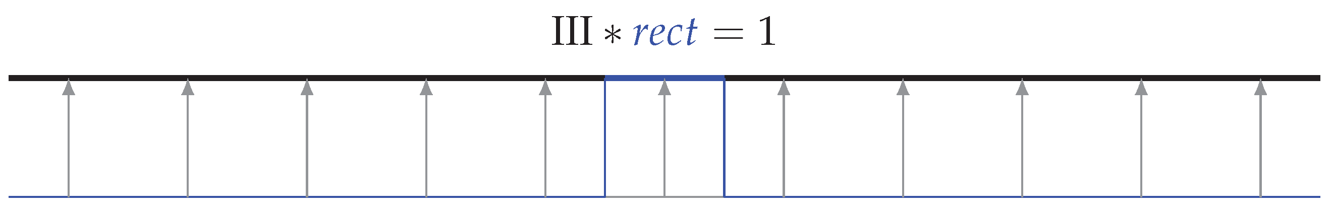
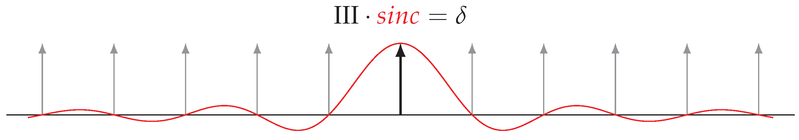
4.1. Single-Sided Partitions of Unity

Dirac combs play a double role. Convolutions with them periodize functions and multiplications with them discretize functions [51,60,61]. In order to reverse these operations, we need to find the convolution and multiplication inverses of Dirac combs in S . Before getting deeper into this topic, let us make the following intriguing observation.
Lemma 4
(Single-Sided Partitions of Unity). There are generalized functions Ω S such that
III Ω = 1
III · Ω ^ = δ
hold simultaneously in the tempered distributions sense.
Proof. 
One may choose Ω r e c t and Ω ^ s i n c as r e c t O C , s i n c O M and III S fulfill Lemma 1. Hence, the equalities (9) and (10) hold in S . □
Obviously, (9) and (10) are Fourier transforms of one another. In Figure 2 and Figure 3 we illustrate this particular solution (cf. Table 1 in [59], Rules 19 and 20). However, the reversal is not true. Choosing, vice versa Ω s i n c and Ω ^ r e c t , both products (9) and (10) do not exist in S (Remark 2 in [59]). It is implied by the fact that r e c t is not smooth ( r e c t O M ) and, equivalently, s i n c is not rapidly decreasing ( s i n c O C ) but slowly decreasing (e.g., Forster [71], p. 106).
As a result of this, the classical Whittaker–Kotel’nikov–Shannon (WKS) sampling theorem [79,80,81], which relies on its s i n c -function reconstruction formula, fails most generally ([40], p. 357 and [79], p. 627). It is, however, true on Lebesgue-square integrable functions (which are rapidly decreasing).

4.2. Double-Sided Smooth Partitions of Unity

The property not being possessed by the Fourier transform pair { r e c t , s i n c } is the circumstance that if Ω and Ω ^ satisfy (9) and (10), then Ω ^ and Ω should satisfy (9) and (10) as well. In other words, the pair { Ω , Ω ^ } should be able to swap roles. The fact that this can indeed be done may be seen in Figure 2 where r e c t is already local (compact support) but needs to be regularized (smooth) at its boundaries, and equivalently, s i n c is already regular (smooth) but needs to be localized at the origin [58]. In other words, we need to have "smooth partitions of unity" in both, time and frequency.
Lemma 5
(Double-Sided Smooth Partitions of Unity). There are Ω S , satisfying Ω Ω ^ , such that
III Ω = 1 = Ω ^ III
III · Ω ^ = δ = Ω · III
hold simultaneously in the tempered distributions sense.
Proof. 
The left-hand side in (11) is a condition fulfilled by any unitary function Ω D and the right-hand side in (12) is additionally satisfied if Ω ( 0 ) = 1 and Ω ( k ) = 0 for any integer k 0 . The other two equations are instantaneously satisfied by the Fourier transform Ω ^ Z of Ω D .  □
Unitary functions (Figure 4) were introduced by Lighthill [5], p. 61. A function Ω T ( t ) is said to be a unitary function ([8], p. 315 and [79]) if it is an element in D and if there exists a real number T for which
T Ω T = 1 .
A special case is T = 1 such that Ω = 1 . We moreover call functions Ω T S satisfying
T Ω T = 1 and T Ω T = δ
“double-sided unitary” due to the following Lemma.
Lemma 6
(Reversibility). The Fourier transform of a double-sided unitary function is double-sided unitary.
Proof. 
Let Ω D such that Ω = 1 and Ω = δ , and let Ω T : = Ω ( t / T ) for real T > 0 . First, we observe that F ( Ω T ) = F ( Ω ( t / T ) ) = T Ω ^ ( T t ) = T Ω ^ 1 T . Fourier transforming both sides simultaneously yields, according to Lemma 2,
F ( T Ω T ) = δ and F ( T Ω T ) = 1 1 T 1 T F ( Ω T ) = δ and 1 T 1 T F ( Ω T ) = 1 1 T Ω ^ 1 T = δ and 1 T Ω ^ 1 T = 1 .
Hence, Ω ^ 1 T Z is again a double-sided unitary.  □
For this reason, it is a requirement to distinguish between finite ( D ) and entire ( Z ) double-sided unitary functions. Appendix A describes the construction of Ω T D . Let us now generalize Lemma 5 from T = 1 to arbitrary real-valued T > 0 .
Theorem 1
(Cross-Inverses of the Dirac Comb). Let T > 0 be real, Ω T D double-sided unitary; then,
III T Ω T = 1 = Ω ^ 1 T III 1 T
III 1 T · Ω ^ 1 T = δ = Ω T · III T
hold simultaneously in the tempered distributions sense.
Proof. 
Lemma 5, F ( III T ) = 1 T III 1 T and F ( Ω T ) = T Ω ^ 1 T yield the assertion.  □
A comprehensive treatment of unitary functions can be found in Zemanian [8], p. 315 or Boyd [82,83,84], for example. Very similar is the use of distributed approximating functionals (DAF); see, e.g., Figure 1 in Bodmann [85]. Unitary functions form particular partitions of unity which play an important role in functional analysis [17,19,71,81,86,87]. However, Lighthill’s unitary functions are smooth ( O M ) and compactly supported ( O C ), such that we may multiply and convolve them with any tempered distribution (Lemma 1).

4.3. Operations Interpretation

Equations (11), (12), (15) and (16), correspondingly, can be interpreted in many different ways. We now think of one function as an operator which is applied to the other function (see Figure 5). Because double-sided unitary functions are double-sided smooth ( S ), we are allowed to apply them to any tempered distribution ( S ). Vice versa, any tempered distribution can be applied to any Schwartz function. Table 1 lists all operations involved.
There are two operations (discretization, periodization) towards discreteness and four operations (regularization, localization, finitization, entirization) towards smoothness. The latter four reverse the preceding two. Smoothness can be obtained either with smooth (regularization, localization) or with sharp (finitization, entirization) interval boundaries.
All six operations arise in Lemma 5. The equation III Ω = 1 , for example, describes periodization ( Ω ) = 1 and regularization ( III ) = 1 , simultaneously. In Figure 5, we see that (11) can be found on the left and (12) can be found on the right-hand side; both are mapping towards { 1 , δ } . Thus, four operations in Figure 5 represent Lemma 5; they map towards { 1 , δ } , and another four (identity) operations map away from { 1 , δ } . They map towards the poles { Ω ^ , Ω } and { III , III ^ } , respectively.

4.4. Applications

In two preceding studies, we already described the pole of discreteness (Theorem 1 in [57]) and the pole of smoothness (Theorem 1 in [58]) in theorems. One is the duality between discretization and periodization (Poisson’s summation formula) and the other is the duality between regularization and localization (Heisenberg’s uncertainty principle). Altogether, their message is the duality between smoothness and discreteness which can also be found in Lemma 1.
Remark 1
(Arbitrary Products). According to Lemma 1 it is required that at least one of the two factors in multiplication products is a regular function, and equivalently, at least one of the two factors in convolution products is a local function. Hence, using regularization and localization (Table 1), both products
f · g : = f · ϵ g
f g : = f ^ 1 ϵ g
exist for arbitrary f , g S . The entity ϵ > 0 denotes their position accuracy (uncertainty).
A general rule of thumb is that regularity is required for multiplications and locality is required for convolutions. Another consequence of this is the following.
Remark 2
(Square of the Dirac Delta). According to the previous remark, the product
δ · ϵ δ = δ
exists in S . For infinitesimally small ϵ > 0 , it is close to δ · δ which does not exist. However, even for any ϵ > 0 , this product reduces to δ. One may recall that Ω ϵ ( 0 ) = 1 . Hence, δ is an idempotent operator.
Equation (19) regularizes the square of the Dirac delta. The procedure of turning ill-conditioned multiplication products into rigorously defined products is called “renormalization” in quantum physics [30,88,89,90,91]. The regularization here coincides, in fact, with the renormalization (1.10) obtained in [30] except for a constant c. This constant arises due to formula (13) in [35], p. 61.

4.5. Self-Reciprocity

It is interesting to observe that Ω Ω ^ in (11) and (12) implies that these equations collapse from four to only two equations. Hence, requiring Ω Ω ^ (self-reciprocity) means a fallback from Lemma 5 to Lemma 4. We, therefore, conclude the following.
Corollary 1
(Double-sided partitions of unity cannot be self-reciprocal). There is no function satisfying Ω Ω ^ such that (11) and (12) hold simultaneously in the tempered distributions sense.
By “self-reciprocal” we mean it is the Fourier transform of itself [92,93,94,95,96]. Because only one of the two factors ( Ω , III ) in (11) and (12) can be self-reciprocal and because III is self-reciprocal, Ω cannot be self-reciprocal.
Corollary 2
(Double-headed Pole). The pole of smoothness is double-headed { Ω , Ω ^ } in contrast to the pole of discreteness which is single-headed { III } .
“Double-headed” means two functions { Ω , Ω ^ } are required to pull tempered distributions towards the pole of smoothness (Figure 5). In contrast to this, only one function { III } is needed to pull them towards the pole of discreteness. There are of course Schwartz functions satisfying Ω Ω ^ such as the Gaussian or the Hyperbolic secant [58], but they cannot be smooth double-sided partitions of unity simultaneously. These two properties, being a smooth double-sided partition of unity and being self-reciprocal, are just mutually exclusive.

5. Outlook

We have seen that two operations ( III · , III ) applied to tempered distributions (discretization, periodization) may be neutralized by four counter-operations ( Ω , Ω ^ · , Ω · , Ω ^ ) applied to these tempered distributions (regularization, localization, finitization, entirization). This is an important property of smooth double-sided unitary functions ( Ω , Ω ^ ) which will be needed in later studies. Figure 5 merely depicts these operations on simple functions ( Ω , 1 , δ , III ). These operations, however, have the potential to reverse more general discretizations or periodizations applied to tempered distributions. We will show that simple symbolic calculation rules apply. The classical sampling theorem then appears in an entirely new light.

Author Contributions

Conceptualization, J.V.F.; methodology, J.V.F.; software, J.V.F.; validation, J.V.F. and R.L.S.; formal analysis, J.V.F.; investigation, J.V.F.; writing—original draft preparation, J.V.F.; writing—review and editing, J.V.F. and R.L.S.; visualization, J.V.F.; supervision, R.L.S.

Funding

This research received no external funding. Its publication is financially supported by the German Aerospace Center (DLR)’s dedicated fond for Open Access publishing.

Acknowledgments

The authors would like to thank the reviewers for their thorough review, further hints to the literature and very constructive comments.

Conflicts of Interest

The authors declare no conflicts of interest.

Appendix A. Construction of Unitary Functions

Appendix A.1. Construction via Integration

Let ϵ > 0 and ϕ ( t ) = e 1 / ( 1 ( t / ( 2 ϵ ) ) 2 ) / + e 1 / ( 1 ( t / ( 2 ϵ ) ) 2 ) d t for ϵ / 2 < t < + ϵ / 2 and zero else. Then ϕ D , its integral is 1 and its support is ϵ / 2 , + ϵ / 2 . It constructs the derivative
d d t Ω T : = ϕ T / 2 ϕ + T / 2
where ϕ a ( τ ) : = ϕ ( τ a ) and T ϵ , of a unitary function (Figure 4)
Ω T ( t ) = t ( d d t Ω T ) ( τ ) d τ
such that 1 T + Ω T = 1 , T Ω T = 1 and T Ω T = δ . Hence, Ω T D is double-sided unitary.

Appendix A.2. Construction via Regularization

Equivalently, one may let Ω T : = ϕ ( r e c t T ) , where ϕ f : = ϕ f is called regularization [58] of f S , r e c t T ( t ) : = r e c t ( t / T ) is the rectangular function with support T / 2 , + T / 2 and ϕ is a mollifier [18,38,39], also called regularizer [97,98]. It can easily be seen that this is an equivalent construction of Ω T because
d d t Ω T = d d t ϕ ( r e c t T ) = d d t ( ϕ r e c t T ) = ϕ d d t ( r e c t T ) = ϕ ( δ T / 2 δ + T / 2 )
equals (A1). The rule d d t ( f g ) = f ( d d t g ) = ( d d t f ) g is commonly known and 1 T ( δ T / 2 δ + T / 2 ) is the derivative of δ for T 0 .

References

  1. Schwartz, L. Théorie des Distributions, Tome I; Hermann: Paris, France, 1950. [Google Scholar]
  2. Schwartz, L. Théorie des Distributions, Tome II; Hermann: Paris, France, 1951. [Google Scholar]
  3. Halperin, I.; Schwartz, L. Introduction to the Theory of Distributions; University of Toronto Press, Scholarly Publishing: Toronto, ON, Canada, 1952. [Google Scholar]
  4. Temple, G. The Theory of Generalized Functions. Proc. R. Soc. Lond. Ser. A. Math. Phys. Sci. 1955, 228, 175–190. [Google Scholar]
  5. Lighthill, M.J. An Introduction to Fourier Analysis and Generalised Functions; Cambridge University Press: Cambridge, UK, 1958. [Google Scholar]
  6. Erdélyi, A. Operational Calculus and Generalized Functions; Holt, Rinehart and Winston, Inc.: New York, NY, USA, 1962. [Google Scholar]
  7. Gel’fand, I.M.; Vilenkin, N.Y. Generalized Functions: Applications of Harmonic Analysis; Academic Press: New York, NY, USA, 1964; Volume 4. [Google Scholar]
  8. Zemanian, A. Distribution Theory And Transform Analysis—An Introduction to Generalized Functions, with Applications; McGraw-Hill Inc.: New York, NY, USA, 1965. [Google Scholar]
  9. Horváth, J. Topological Vector Spaces and Distributions; Addison-Wesley Publishing Company: Reading, MA, USA, 1966. [Google Scholar]
  10. Jones, D. The Theory of Generalized Functions; Cambridge University Press: Cambridge, UK, 1966. [Google Scholar]
  11. Trèves, F. Topological Vector Spaces, Distributions and Kernels: Pure and Applied Mathematics; Dover Publications Inc.: Mineola, NY, USA, 1967; Volume 25. [Google Scholar]
  12. Zemanian, A. An Introduction to Generalized Functions and the Generalized Laplace and Legendre Transformations. SIAM Rev. 1968, 10, 1–24. [Google Scholar] [CrossRef]
  13. Zemanian, A.H. Generalized Integral Transformations; Dover Publications Inc.: Mineola, NY, USA, 1968. [Google Scholar]
  14. Gel’fand, I.; Schilow, G. Verallgemeinerte Funktionen (Distributionen), Teil I-II; Deutscher Verlag der Wissenschaften: Berlin, Germany, 1969. [Google Scholar]
  15. Ehrenpreis, L. Fourier Analysis in Several Complex Variables; John Wiley & Sons, Inc.: Mineola, NY, USA, 1970. [Google Scholar]
  16. Vladimirov, V.S. Gleichungen der Mathematischen Physik; Deutscher Verlag der Wissenschaften: Berlin, Germany, 1972. [Google Scholar]
  17. Barros-Neto, J. An Introduction to the Theory of Distributions; Marcel Dekker Inc.: New York, NY, USA, 1973. [Google Scholar]
  18. Peterson, B.E. Introduction to the Fourier Transform and Pseudo-Differential Operators; Pitman Publishing Inc.: Marshfield, MA, USA, 1983. [Google Scholar]
  19. Hörmander, L. The Analysis of Linear Partial Differential Operators I, Die Grundlehren der Mathematischen Wissenschaften; Springer: Berlin/Heidelberg, Germany, 1983. [Google Scholar]
  20. Hoskins, R.F.; Pinto, J.S. Distributions, Ultradistributions and Other Generalized Functions; Woodhead Publishing Ltd.: Cambridge, UK, 1994. [Google Scholar]
  21. Walter, W. Einführung in die Theorie der Distributionen; BI-Wissenschaftsverlag, Bibliographisches Institut & FA Brockhaus: Mannheim, Germany, 1994. [Google Scholar]
  22. Zayed, A.I. Handbook of Function and Generalized Function Transformations; CRC Press Inc.: Boca Raton, FL, USA, 1996. [Google Scholar]
  23. Vladimirov, V.S. Methods of the Theory of Generalized Functions; CRC Press Inc.: Boca Raton, FL, USA, 2002. [Google Scholar]
  24. Strichartz, R.S. A Guide to Distribution Theory and Fourier Transforms; World Scientific Publishing Co. Pte Ltd.: Singapore, 2003. [Google Scholar]
  25. Rahman, M. Applications of Fourier Transforms to Generalized Functions; WIT Press: Southampton, UK, 2011. [Google Scholar]
  26. Mikusiński, J. On the square of the Dirac delta-distribution. Bull. de l’Acad. Pol. Sci. Sér. Sci. Math. Astr. Phys. 1966, 14, 511–513. [Google Scholar]
  27. Koh, E.; Li, C. On defining the generalized functions δα(z) and δn(x). Int. J. Math. Math. Sci. 1993, 16, 749–754. [Google Scholar] [CrossRef]
  28. Özçağ, E. Defining the k-th Powers of the Dirac-Delta Distribution for Negative Integers. Appl. Math. Lett. 2001, 14, 419–423. [Google Scholar] [CrossRef] [Green Version]
  29. Li, C. A Review on the Products of Distributions. In Mathematical Methods in Engineering; Springer: Dordrecht, The Netherlands, 2007; pp. 71–96. [Google Scholar]
  30. Accardi, L.; Boukas, A. Powers of the Delta Function. In Quantum Probability and Infinite Dimensional Analysis; World Scientific Publishing Co. Pte. Ltd.: Singapore, 2007; pp. 33–44. [Google Scholar]
  31. Kiliçman, A. Note on the Products of Distributions. Math Dig. Res. Bull. Inst. Math. Res. 2008, 1, 1–5. [Google Scholar]
  32. Li, C. The Powers of the Dirac Delta Function by Caputo Fractional Derivatives. J. Fract. Calc. Appl. 2016, 7, 12–23. [Google Scholar]
  33. Özçağ, E. Results on Compositions Involving Dirac-Delta Function; AIP Conference Proceedings; AIP Publishing: Melville, NY, USA, 2017; Volume 1895, p. 050007. [Google Scholar]
  34. Özçağ, E. On Powers of the Compositions Involving Dirac-Delta and Infinitely Differentiable Functions. Results Math. 2018, 73, 6. [Google Scholar] [CrossRef]
  35. Dirac, P. The Principles of Quantum Mechanics; Oxford University Press: Oxford, UK, 1930. [Google Scholar]
  36. Córdoba, A. Dirac Combs. Lett. Math. Phys. 1989, 17, 191–196. [Google Scholar] [CrossRef]
  37. Oberguggenberger, M.B. Multiplication of Distributions and Applications to Partial Differential Equations; Longman Scientific & Technical: Harlow, UK, 1992; Volume 259. [Google Scholar]
  38. Friedrichs, K.O. On the Differentiability of the Solutions of Linear Elliptic Differential Equations. Commun. Pure Appl. Math. 1953, 6, 299–326. [Google Scholar] [CrossRef]
  39. Schechter, M. Modern Methods in Partial Differential Equations, An Introduction; McGraw-Hill Book Company: New York, NY, USA, 1977. [Google Scholar]
  40. Gasquet, C.; Witomski, P. Fourier Analysis and Applications: Filtering, Numerical Computation, Wavelets; Springer Science & Business Media: New York, NY, USA, 1999; Volume 30. [Google Scholar]
  41. Simon, B. Distributions and their Hermite Expansions. J. Math. Phys. 1971, 12, 140–148. [Google Scholar] [CrossRef]
  42. Reed, M.; Simon, B. II: Fourier Analysis, Self-Adjointness; Academic Press Inc.: New York, NY, USA, 1975; Volume II. [Google Scholar]
  43. Folland, G.B. Harmonic Analysis in Phase Space; Princeton University Press: Princeton, NJ, USA, 1989. [Google Scholar]
  44. Messiah, A. Quantum Mechanics—Two Volumes Bound as One; Dover Publications: New York, NY, USA, 2003. [Google Scholar]
  45. Mund, J.; Schroer, B.; Yngvason, J. String-Localized Quantum Fields from Wigner Representations. Phys. Lett. B 2004, 596, 156–162. [Google Scholar] [CrossRef] [Green Version]
  46. Glimm, J.; Jaffe, A. Quantum Physics: A Functional Integral Point of View; Springer-Verlag Inc.: New York, NY, USA, 2012. [Google Scholar]
  47. de Costa Campos, L.M.B. Generalized Calculus with Applications to Matter and Forces; CRC Press: Boca Raton, FL, USA, 2014. [Google Scholar]
  48. Bahns, D.; Doplicher, S.; Morsella, G.; Piacitelli, G. Quantum Spacetime and Algebraic Quantum Field Theory. In Advances in Algebraic Quantum Field Theory; Springer: Cham, Switzerland, 2015; pp. 289–330. [Google Scholar]
  49. Li, C.; Li, C.; Humphries, T.; Plowman, H. Remarks on the Generalized Fractional Laplacian Operator. Mathematics 2019, 7, 320. [Google Scholar] [CrossRef] [Green Version]
  50. Dierolf, P. The Structure Theorem for Linear Transfer Systems. Note Mat. 1991, 11, 119–125. [Google Scholar]
  51. Osgood, B. The Fourier Transform and Its Applications; EE 261 Lecture Notes; Stanford University: Stanford, CA, USA, 2007. [Google Scholar]
  52. Süße, H.; Rodner, E. Bildverarbeitung und Objekterkennung; Springer: Wiesbaden, Germany, 2014. [Google Scholar]
  53. Smith, D.C. An Introduction to Distribution Theory for Signals Analysis. Digit. Signal Process. 2006, 16, 419–444. [Google Scholar] [CrossRef]
  54. Burger, W.; Burge, M.J. Digital Image Processing: An Algorithmic Introduction Using Java; Springer-Verlag: London, UK, 2016. [Google Scholar]
  55. Lützen, J. The Prehistory of the Theory of Distributions; Vol. 7, Studies in the History of Mathematics and Physical Sciences; Springer: Berlin/Heidelberg, Germany, 1982. [Google Scholar]
  56. Debnath, L. A Short Biography of Paul A M Dirac and Historical Development of Dirac Delta Function. Int. J. Math. Educ. Sci. Technol. 2013, 44, 1201–1223. [Google Scholar] [CrossRef]
  57. Fischer, J.V. On the Duality of Discrete and Periodic Functions. Mathematics 2015, 3, 299–318. [Google Scholar] [CrossRef] [Green Version]
  58. Fischer, J.V. On the Duality of Regular and Local Functions. Mathematics 2017, 5, 41. [Google Scholar] [CrossRef] [Green Version]
  59. Fischer, J.V. Four Particular Cases of the Fourier Transform. Mathematics 2018, 6, 335. [Google Scholar] [CrossRef] [Green Version]
  60. Bracewell, R.N. Fourier Transform and its Applications; McGraw-Hill Book Company: New York, NY, USA, 1986. [Google Scholar]
  61. Kammler, D.W. A First Course in Fourier Analysis; Cambridge University Press: Cambridge, UK, 2007. [Google Scholar]
  62. Sebastião e Silva, J. Les fonctions analytiques comme ultra-distributions dans le calcul opérationnel. Math. Ann. 1958, 136, 58–96. [Google Scholar] [CrossRef]
  63. Bengel, G. Das Weylsche Lemma in der Theorie der Hyperfunktionen. Math. Z. 1967, 96, 373–392. [Google Scholar] [CrossRef] [Green Version]
  64. Bényi, Á.; Grafakos, L.; Gröchenig, K.; Okoudjou, K. A Class of Fourier Multipliers for Modulation Spaces. Appl. Comput. Harmon. Anal. 2005, 19, 131–139. [Google Scholar] [CrossRef] [Green Version]
  65. Bényi, Á.; Gröchenig, K.; Okoudjou, K.A.; Rogers, L.G. Unimodular Fourier Multipliers for Modulation Spaces. J. Funct. Anal. 2007, 246, 366–384. [Google Scholar] [CrossRef] [Green Version]
  66. Cordero, E.; Trapasso, S.I. Linear Perturbations of the Wigner Distribution and the Cohen’s Class. arXiv 2018, arXiv:1811.07795. [Google Scholar]
  67. Bayer, D.; Cordero, E.; Gröchenig, K.; Trapasso, S.I. Linear Perturbations of the Wigner Transform and the Weyl Quantization. arXiv 2019, arXiv:1906.02503. [Google Scholar]
  68. Kaplan, W. Operational Methods for Linear Systems; Addison-Wesley Pub. Co.: Boston, MA, USA, 1962. [Google Scholar]
  69. Chandrasekharan, K. Classical Fourier Transforms; Springer: Berlin/Heidelberg, Germany, 1989. [Google Scholar]
  70. Fischer, J. Anwendung der Theorie der Distributionen auf ein Problem in der Signalverarbeitung. Diploma Thesis, Ludwig-Maximillians-Universität München, Fakultät für Mathematik, Munich, Germany, 1997. [Google Scholar]
  71. Forster, O. Analysis 3, Integralrechnung im IRn mit Anwendungen, 3. Auflage; Vieweg: Wiesbaden, Germany, 1984. [Google Scholar]
  72. Hasumi, M. Note on the n-dimensional Tempered Ultra-Distributions. Tohoku Math. J. Second Ser. 1961, 13, 94–104. [Google Scholar] [CrossRef]
  73. Kiliçman, A. Generalized Functions Using the Neutrix Calculus. Ph.D. Thesis, University of Leicester, Leicester, UK, 1995. [Google Scholar]
  74. Berenstein, C.A.; Gay, R. Exponential Polynomials. In Complex Analysis and Special Topics in Harmonic Analysis; Springer: New York, NY, USA, 1995. [Google Scholar]
  75. Mikusiński, J. Irregular Operations on Distributions. Stud. Math. 1961, 20, 163–169. [Google Scholar] [CrossRef] [Green Version]
  76. Kamiński, A. Convolution, Product and Fourier Transform of Distributions. Stud. Math. 1982, 74, 83–96. [Google Scholar] [CrossRef]
  77. Gruber, M. Proofs of the Nyquist-Shannon Sampling Theorem. Bachelor’s Thesis, University Konstanz, Konstanz, Germany, 2013. [Google Scholar]
  78. Woodward, P.M. Probability and Information Theory, with Applications to Radar; Pergamon Press Ltd.: Oxford, UK, 1953. [Google Scholar]
  79. Campbell, L. Sampling Theorems for the Fourier Transform of a Distribution with Bounded Support. SIAM J. Appl. Math. 1968, 16, 626–636. [Google Scholar] [CrossRef]
  80. Lüke, H.D. The Origins of the Sampling Theorem. IEEE Commun. Mag. 1999, 37, 106–108. [Google Scholar] [CrossRef] [Green Version]
  81. Unser, M. Sampling-50 Years after Shannon. Proc. IEEE 2000, 88, 569–587. [Google Scholar] [CrossRef] [Green Version]
  82. Boyd, J.P. Construction of Lighthill’s Unitary Functions: The Imbricate Series of Unity. Appl. Math. Comput. 1997, 86, 1–10. [Google Scholar] [CrossRef]
  83. Boyd, J.P. Asymptotic Fourier Coefficients for a C Bell (Smoothed-”Top-Hat”) & the Fourier Extension Problem. J. Sci. Comput. 2006, 29, 1–24. [Google Scholar]
  84. Termonia, P.; Voitus, F.; Degrauwe, D.; Caluwaerts, S.; Hamdi, R. Application of Boyd’s Periodization and Relaxation Method in a Spectral Atmospheric Limited-Area Model. Part I: Implementation and Reproducibility Tests. Mon. Weather Rev. 2012, 140, 3137–3148. [Google Scholar] [CrossRef] [Green Version]
  85. Bodmann, B.G.; Hoffman, D.K.; Kouri, D.J.; Papadakis, M. Hermite Distributed Approximating Functionals as Almost-Ideal Low-Pass Filters. Sampl. Theory Signal Image Process. 2008, 7, 15. [Google Scholar]
  86. Feichtinger, H.G. Banach Convolution Algebras of Wiener Type. Funct. Ser. Oper. Proc. Conf. Bp. 1980, 38, 509–524. [Google Scholar]
  87. Ionescu-Tira, M. Time-Frequency Analysis in the Unit Ball. arXiv 2019, arXiv:1905.03178. [Google Scholar]
  88. Bogolyubov, N.N.; Shirkov, D. Introduction to the Theory of Quantized Fields. Intersci. Monogr. Phys. Astron. 1980, 3, 1–720. [Google Scholar] [CrossRef]
  89. Accardi, L.; Boukas, A. The Emergence of the Virasoro and w Algebras through the Renormalized Higher Powers of Quantum White Noise. arXiv 2006, arXiv:math-ph/0607062. [Google Scholar]
  90. Accardi, L.; Boukas, A. Renormalized Higher Powers of White Noise (RHPWN) and Conformal Field Theory. Infinite Dimens. Anal. Quantum Probab. Relat. Top. 2006, 9, 353–360. [Google Scholar] [CrossRef] [Green Version]
  91. Accardi, L.; Boukas, A. Quantum Probability, Renormalization and Infinite Dimensional ∗–Lie Algebras. Symm. Integrab. Geom. Methods Appl. 2009, 5, 056. [Google Scholar] [CrossRef] [Green Version]
  92. Hardy, G.H.; Titchmarsh, E. Self-Reciprocal Functions. Q. J. Math. 1930, 9, 196–231. [Google Scholar] [CrossRef]
  93. Born, M. A Suggestion for Unifying Quantum Theory and Relativity. J. Chem. Phys. 1938, 3, 439–444. [Google Scholar] [CrossRef] [Green Version]
  94. Born, M. Reciprocity Theory of Elementary Particles. Rev. Mod. Phys. 1949, 21, 463. [Google Scholar] [CrossRef] [Green Version]
  95. Cowley, J.; Moodie, A. Fourier Images: II-The Out-of-focus Patterns. Proc. Phys. Soc. Sect. B 1957, 70, 497. [Google Scholar] [CrossRef]
  96. de Branges, L. Self-Reciprocal Functions. J. Math. Anal. Appl. 1964, 9, 433–457. [Google Scholar] [CrossRef] [Green Version]
  97. Wei, G. Quasi Wavelets and Quasi Interpolating Wavelets. Chem. Phys. Lett. 1998, 296, 215–222. [Google Scholar] [CrossRef]
  98. Wei, G.W.; Gu, Y. Conjugate Filter Approach for Solving Burgers’ Equation. J. Comput. Appl. Math. 2002, 149, 439–456. [Google Scholar] [CrossRef]
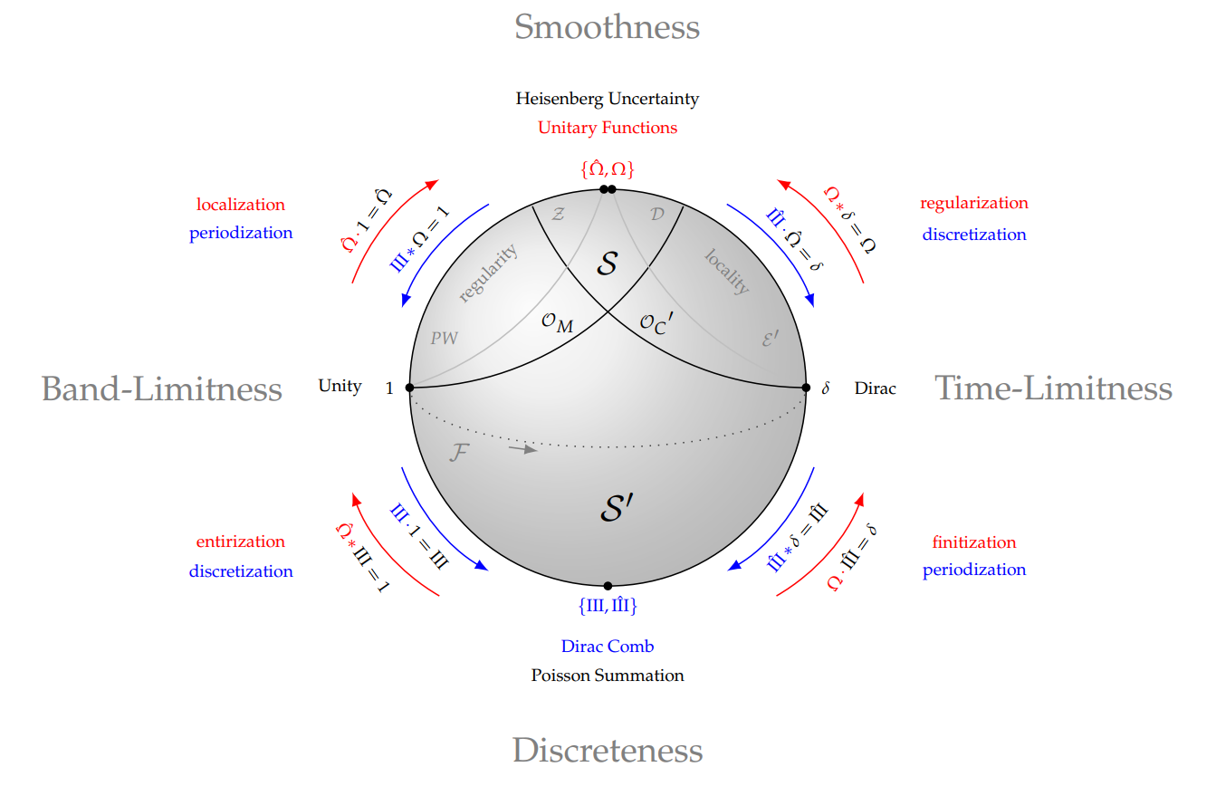
 [Green Version]
Figure 1. The space of tempered distributions and important subspaces.
Mathematics 07 01196 g001
Figure 2. In contrast to III r e c t the product III · r e c t does not exist in S .
Mathematics 07 01196 g002
Figure 3. In contrast to III · s i n c the product III s i n c does not exist in S .
Mathematics 07 01196 g003
Figure 4. Both products III T Ω T = 1 and III T · Ω T = δ exist in S .
Mathematics 07 01196 g004
Figure 5. Operations towards smoothness (red) reverse operations towards discreteness (blue).
Mathematics 07 01196 g005
Table 1. Operations from smoothness towards discreteness and vice versa.
NoOperationDomainDefinitionGoalResultFunction
IDiscretization f O M T f : = III · f Discreteness (time) T f S discrete
IIPeriodization f O C T f : = III f Discreteness (freq) T f S periodic
(i)Regularization f S T f : = Ω T f Smoothness (time), smooth T f O M regular
(ii)Localization f S ^ T f : = Ω ^ T · f Smoothness (freq), smooth ^ T f O C local
[i]Finitization f S T f : = Ω T · f Smoothness (freq), sharp T f E finite
[ii]Entirization f S ^ T f : = Ω ^ T f Smoothness (time), sharp ^ T f P W entire

