Evolutionary Game Analysis on Strategies in “Main Manufacturer–Supplier” Mode Considering Technology Docking and Price Concluding under Competition Condition

Abstract

This paper analyses the strategies of the substitutable suppliers competing to collaborate with a main manufacturer in “main manufacturer–supplier” (M-S) mode. In the research and development (R&D) of complex products, only one supplier can be chosen for one kind of part as a long-term collaboration partner with the manufacturer. The competition between substitutable suppliers focuses on the technology docking and price-concluding strategies. In this paper, one original supplier as the first-mover and one new supplier as the second-mover chose between the two strategies sequentially to compete for the collaborative preference of the manufacturer. We also took the delay cost brought by strategy changing into the consideration of the risks, which the suppliers and the manufacturer should prepare to share. With evolutionary game theory applied, we can conclude that the initial costs have little impact on suppliers’ making decisions, while the initial prices are correlated with both suppliers’ decision making. Results also show that hesitation and fluctuation periods exist in suppliers’ decision making, which have a relationship with existing strategy conditions, initial prices, and the cost caused by modifying the part. These results provide practical and reasonable managerial implications for M-S collaboration.

1. Introduction

The commitment by Boeing Field about the 737 MAX’s safety “going-around” on 17 April 2019 has attracted attention to the cooperation between the Boeing and its partners, its suppliers. Actually, some complex products like big passenger aircrafts, large-scale communication systems, aerospace systems, large ships, power network control systems, high-speed trains, and large-scale weapons and equipment [1] are developed in a so-called “main manufacturer–supplier” (M-S) mode. These kinds of products have the characteristics of high research and development (R&D) cost, large scale, high technology content, single or small batch customization, and high integration. According to the theory of comparative advantage [2], it is economical for the manufacturer to be mainly responsible for the overall design and assembly of the end product, and to outsource the parts of the product to its suppliers. The parts of complex products are also complex, such as the engines of large passenger aircrafts. Suppliers provide the parts they have designed that are closest to the manufacturer’s requirements to the manufacturer. M-S mode requires the manufacturer and the supplier to collaborate in the whole R&D process of the product, work together when problems arise in the production process, and share the risk [3]. For example, for Airbus 380, Airbus designed the drawings of spare parts, formulated technical specifications, and detailed interfaces between modules, while suppliers processed according to these drawings. Then, Airbus purchased spare parts and assembled them into the whole product without the knowledge of how the spare parts were made. Airbus only has to make sure that the spare parts fit the design parameters of the end product. How to manage the suppliers is a big challenge for the manufacturer. Besides, due to the complexity of the complex product itself as well as the R&D process, the collaboration risk and payoff, which should be shared by both the manufacturer and its suppliers, are very difficult, but practical, to quantitatively depict.

Traditionally, due to the characteristic of single or small batch customization of complex products, the manufacturer chooses one supplier for one part of the product as a long-term partnership. Enhancing long-term strategic cooperative positions with suppliers is the best choice for the manufacturer of a complex product. However, increasing competition between alternative suppliers may arise for the manufacturer of a complex product. With the development of economy and society, material demand is developing towards multihabitation. Complex products are gradually developing towards more kinds of service needs. Manufacturers may gain more payoffs from services and support by changing their relationships with suppliers. For example, in order to ensure the reliability of the product and meet the high production speed of its 737 project, Boeing cancelled its contract with GKN Company, the supplier of the 737 MAX aircraft engine thrust device, and instead adopted the Leap-1B engine made by CFM International Company, without affecting the performance of 737 MAX or the plan of first flight, certification, and delivery. The replacement of suppliers was done to solve the potential problem of titanium alloy parts production. Therefore, despite the long-term cooperative relationship between the manufacturer and the supplier, supplier selection and replacement is still one of the issues that the manufacturer must consider in supplier management. Competition still exists between suppliers of complex products, especially for the substitutable suppliers.

Actually, technology and price have always been the primary consideration of the manufacturer when choosing its suppliers. Thus, technology docking and price-concluding strategies are taken into the consideration of the substitutable suppliers’ competition in our paper. Actually, for complex products, especially the aircraft, most of the key technologies come from suppliers, such as engines, electronic systems, and so on. However, suppliers sell their end product and the relevant service to the manufacturer instead of the key technology. For example, on the 787 project, Boeing made its first try with the strategy of global supply chain and only needed to work with 23 first-class suppliers in the world besides its own factories. The number of core suppliers is much smaller than in the past, while the number of outsourcing partners has increased substantially. Therefore, some suppliers not only need to complete the production of components and systems, but also the integration of related components and systems, and then hand assembly to Boeing. However, this first try with the new strategy has brought the announcement of five delays in delivery on Project 787. The suppliers have to spend time on the adjustment of either their parts’ price or technology to meet the requirements of the manufacturing. To the best of our knowledge, while some original suppliers have some collaboration experience and technical advantages, new suppliers can bring more new ideas to adapt to the times. Price is also the key to supplier competition, which is beyond doubt.

We can see that in M-S mode, the manufacturer is responsible for not only the overall design of the end product, but selecting suppliers, managing, and coordinating the relationship between suppliers. Thus, the manufacturer’s preferences is the crucial factor for the suppliers when considering enhancing their own competitiveness. According to the latest global procurement theory [4], procurement management not only pays attention to the procurement execution process, but also pays attention to the management of procurement resources, that is, the management of the potential supplier pool and the management of supplier access, which puts forward higher requirements for supplier selection management. We have considered the manufacturer’s preferences as part of the factors in the competition of the alternative suppliers in this paper.

The risk of delay cost is also the most important concern for both the manufacturers and the suppliers of complex products in our paper. For example, Boeing and its suppliers have to bear the heavy losses due to the delayed delivery caused by the supplier management reform in the 787 project. Moreover, according to the Wall Street Journal, the uncertainties caused by Boeing’s continued grounding of its 737 MAX aircraft have caused untold suffering to its suppliers. More than 600 suppliers relying on Boeing orders are preparing for possible changes in production in case 737 MAX remains grounded. Therefore, the delay cost should not only be the primary concern for the manufacturer when choosing a supplier as its partner, but also be the inevitable concern for the suppliers when choosing the way to compete for the collaboration with the manufacturer. The consideration of delay cost is the biggest difference between complex products and ordinary products.

In order to study the competition between the substitutable suppliers considering the collaborative main manufacturer in the R&D of complex products, we used modeling and simulation theory in this paper. Considering the characteristics of bounded rationality of decision-makers in real life, especially for the substitutable suppliers in the long-term competition in the R&D of complex product, whose cognitive and computational ability are limited, we made an attempt at evolutionary game theory to examine the following issues: (1) How do suppliers choose to collaborate with the manufacturer, depending on price-concluding advantage or technology docking advantage? Our work considered the decision sequence of the two suppliers when modeling their payoff matrix. The original supplier is supposed to have priority over the new supplier in decision-making. This also added difficulty to the following game analysis. (2) Whether the initial prices of suppliers has an impact on the way suppliers choose to collaborate, especially with the consideration of the manufacturer preference and the delay cost? Our work analyzed how the relationship between the initial price of the original supplier and that of the new supplier influence the decision making process. During the analysis, we found that the discussion on the manufacturer’s preferences and the delay cost became the priori basis of our research, which is another essential and difficult part in the game analysis. (3) How do costs influence the collaboration between the manufacturer and the supplier, and the competition between the substitutable suppliers? Our work tried to find the connection between the costs—the initial costs, the delay costs, and the cost brought by suppliers taking measures—and the decision making process, which is very practical in reality but difficult during game analysis. The fact that there are many equilibrium conditions in the game system increased the complexity of the research.

The remainder of the paper is organized as follows. Section 2 provides a review of the related literature, and Section 3 details our modeling assumptions. Section 4 presents our analysis of the final states of the substitutable suppliers as well as the relative existing conditions, including identification of the impact of the initial prices, the initial costs with consideration of the manufacturer’s preferences, and delay cost. Section 5 offers conclusions and suggestions for future research.

2. Literature Review

Our research lies at the intersection of the bodies of literature on (i) the M-S collaborative mode; (ii) the pricing strategy selection; and (iii) the application of the game theory. Next, we describe how our work relates to the literature in these areas.

In recent years, M-S collaborative mode has attracted considerable theoretical and experimental attention. Actually, the earliest idea about the M-S mode was founded in the paper related to feed manufacturing [5]. In later contributions, researchers explored various aspects in the application of the M-S mode, including technology-related industry [6,7,8], textile and clothing industry [9], environmental sustainability [10,11], and complex product R&D [12,13]. Our work is related to the specific stream of literature on the complex product R&D. In the M-S mode of complex product R&D, both the manufacturer and the supplier not only share the payoff brought by the product, but also share the risk and the cost brought during the process of the R&D [14]. The manufacturer is responsible for the end product design and assembly [15], and the component procurement from the suppliers [16]. Yan et al. also studied how an updated demand forecast affects a manufacturer’s choice in ordering raw materials with consideration of two suppliers—one fast but expensive and the other cheap but slow [17]. Moreover, Chen investigated the coordination mechanism for the supply chain with one manufacturer and multiple competing suppliers in the electronic market, focusing on conventional price-only policies [18]. In contrast to these papers, we focused our work on the procurement preference of the manufacturer and the competition between the substitutable suppliers with consideration of technology docking and price-concluding strategies.

Our study is also related to the literature that explores pricing strategy selection. Pricing strategy has always been the hot topic in the research of supply chains. Cattani et al. analyzed a scenario where a manufacturer with a traditional channel partner opened up a direct channel in competition with the traditional channel, with consideration of the wholesale price and retail price strategies [19]. Xiao and Yang developed a price-service competition model of two supply chains to investigate the optimal decisions of players under demand uncertainty [20]. Hua et al. examined the optimal decisions of delivery lead time and prices in a centralized and a decentralized dual-channel supply chain [21]. Ghosh and Shah studied how greening levels, prices, and payoffs are influenced by supply chain channel structures in which the players cooperate or act individually [22]. Our research focused on the price-concluding strategy combined with the technology docking strategy. Prior research has studied how technology quality efforts affect the manufacturing process [23,24,25,26,27]. The relationship between the payoff in a supply chain, especially for the complex product R&D, and the technology-price strategy should never be neglected. Papers have shown the relationship between the demand function and the factors of price and quality [28,29,30,31]. There are also some other papers that have shown the relationship between the cost and the factor of quality [32,33]. Thus, we can then accordingly focus the payoff functions of the players in the M-S mode framework on the price and quality in our work.

Another related body of literature is the research on the application of the evolutionary game theory in the supply chain. Evolutionary game theory is dedicated to research based on the idea that players cannot fully grasp the entirety of the information, and their decision-making will change based on updated knowledge of the information [34]. This kind of game theory has achieved a lot of success in the research of the government enterprise-based low-carbon strategies [35], taxes vs. subsidies problems in the electric vehicle industry [36], and so on. The theory has also combined successfully with the research of the supply chain [37,38,39]. Actually, in the M-S collaborative mode, where the manufacturer tried to establish a new long-term relationship with its suppliers and the substitutable suppliers compete to be the most preference of the manufacturer, information is asymmetric for each of the suppliers. Evolutionary game theory has also helped solve this kind of problem in a collaborative supply chain [40,41]. We focused more on the competition between the substitutable suppliers with the evolutionary game theory.

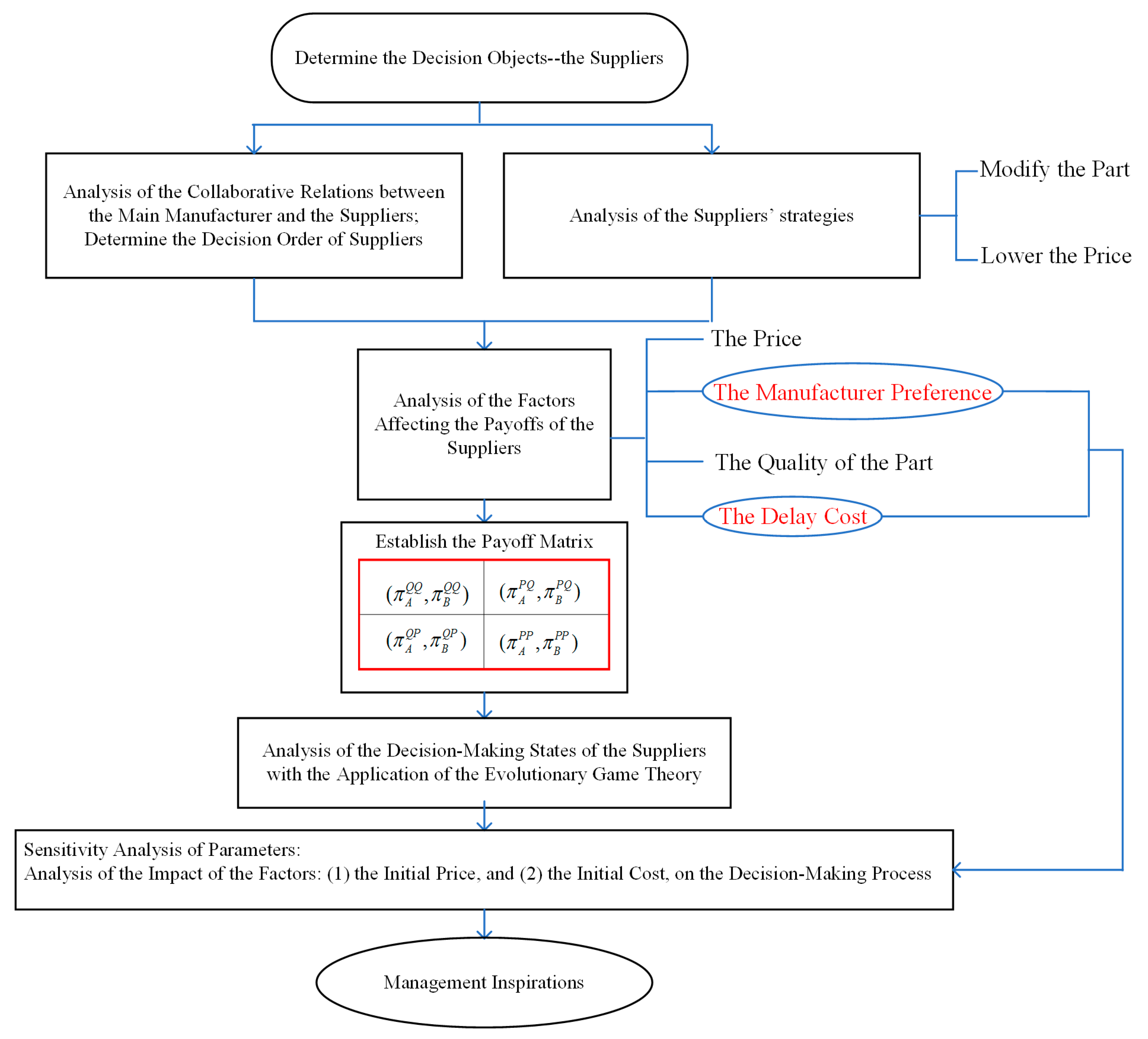
The work presented in this paper therefore borrows elements from the three research streams mentioned above, but differs significantly from previous studies in that it (1) models the problem with evolutionary game theory based on suppliers’ dynamic game; (2) focuses on the inverse selection of suppliers by the main manufacturer who has certain initiative; (3) biases that the main manufacturer makes decisions to respond to supplier-oriented attitudes and prefers to consider improving product quality as a positive attitude, while lowering pricing as a negative cooperative attitude; (4) adds the factor of the delay cost as a characteristic in the R&D of the complex product that differs from that of the ordinary product. The conceptual research model for this paper is shown in Figure 1.

3. Model

To address the research questions posed in Section 1, we conducted a supplier–supplier evolutionary game-playing model, considering the influence of the main manufacturer, with the following features:

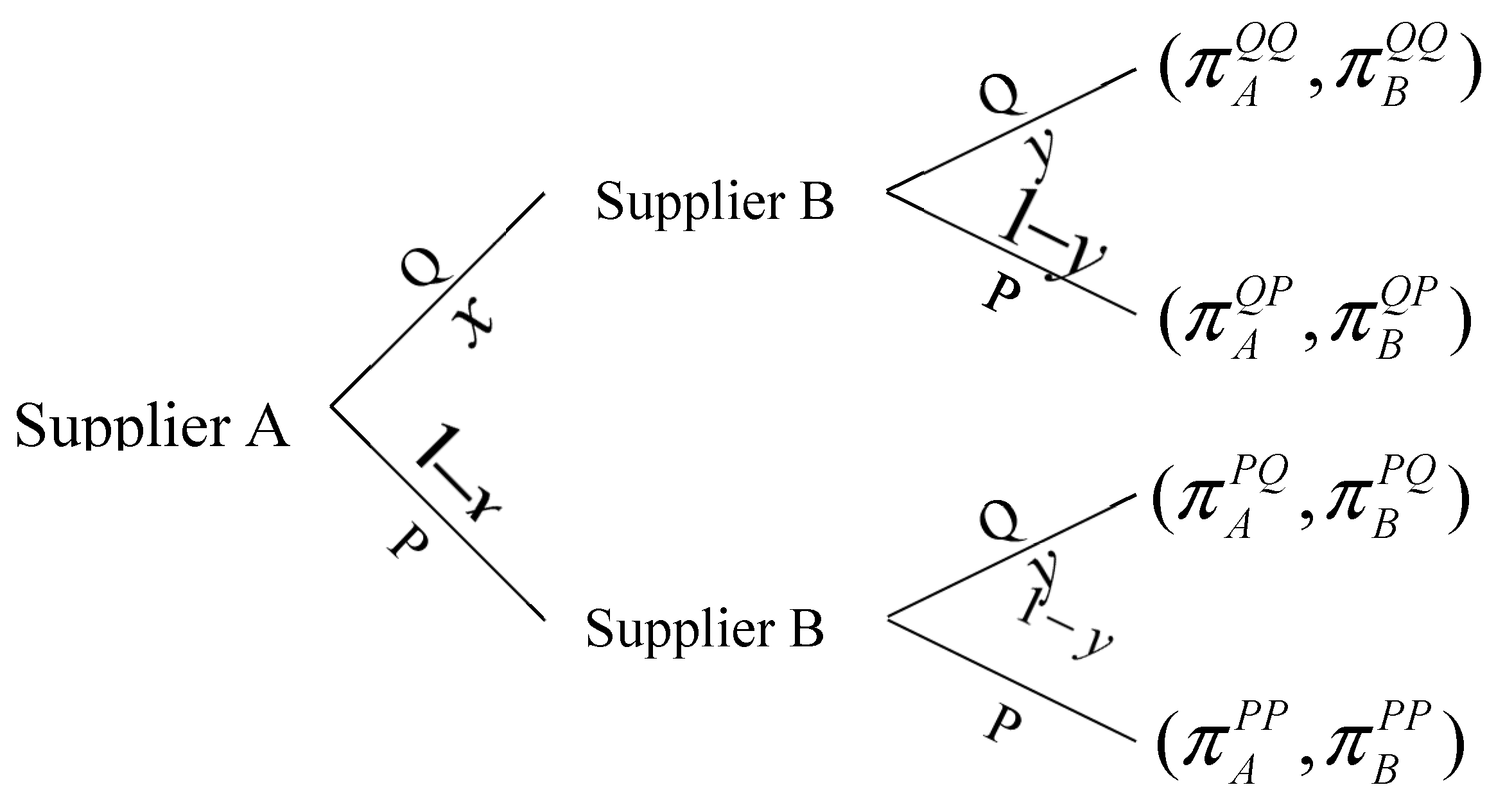
Supply chain structure: We considered a two-echelon supply chain with one original supplier, A, (e.g., the original engine supplier of 737 project, GKN Company) as the first-mover and one new supplier, B, (e.g., the new engine supplier of 737 project, CFM International Company) as the second-mover. Both of them shared the same collaborative R&D mechanism with one downstream manufacturer (e.g., the manufacturer of 737 project, Boeing), and the decision sequence of the two suppliers was assumed to be decided by the manufacturer’s preference in this paper, which is also practical in reality. The manufacturer could choose only one supplier as a long-term partner to collaborate with in a new project designed by the manufacturer (e.g., the establishment of new supplier management system in the project 787) or to reestablish an old project (e.g., the reestablishment of the new M-S relationship in project 737) to meet with the R&D of the manufacturer. The original supplier was assumed to have the priority over the new one because the original one has always had a long-term relationship with the manufacturer. Both suppliers A and B were assumed to be governed by bounded rationality, with limited ability to gather and process information. The part provided by either A or B should have been designed beforehand and the cost of the design is so high that only some strategies should be taken to fit for the requirement of the manufacturer, instead of designing a new one. In this structure, both A and B should have two strategies. As is shown in Figure 2, one strategy is to lower the price of the part provided to the manufacturer within its acceptable range. In this condition, the manufacturer may have to modify the whole design of the product. The other one is to modify the part to fit for the whole design of the final product. But in this way, the cost of the part gets increased. However, as supplier A is assumed to have already kept long-term cooperation with the manufacturer, they have the priority to make this decision over supplier B. The framework is applicable for many collaborative supply chains (e.g., the R&D of a large passenger aircraft) in M-S mode, in which the manufacturer (e.g., COMAC) may have to choose one of the two civil aviation engine suppliers (e.g., GEAE, General Electric Aircraft Engines and Rolls-Royce) for the collaborative R&D of the final product (e.g., the remote wide-body passenger aircraft C929).

As is shown in Figure 2, Q stands for the strategy of modifying the parts, P stands for the strategy of lowering the price, $x$ stands for the probability of supplier A taking the strategy of Q, $y$ stands for the probability of supplier B taking the strategy of Q, and ${\pi }_A^{ij}$ and ${\pi }_B^{ij}$ stand for the payoffs of A and B in the condition of A taking the strategy $i$ and B taking the strategy $j$ ($i$, $j$ = Q, P). Hence, Figure 2 has shown all four strategy conditions for the supply chain, which are shortened to $(QQ,QP,PQ,PP)$. According to Cohen-Vernik and Purohit [42], and Ranjan and Jha [43], the payoff of the supplier should be represented by the following function:

$$\pi =pD(p,q)-C(q,t)$$

(1)

where $p$ is the price of the part, $q$ is the quality of the part, $D$ is the demand level and has the relationship with $p$ and $q$, $t$ is the existing cost on time delay as considered in the model, and $C$ is the cost, which is assumed to have the relationship with $q$ and $t$ in our paper. We have considered the factors of product quality and time cost in the payoff functions, which are different from the traditional payoff function but practical and reasonable in the R&D of complex products. Actually, as the manufacturer only chooses one supplier to cooperate with, we just used the demand level as a representation of the manufacturer preference here instead of the demand quantity. Besides, the cost of time $t$ is a very important consideration in the R&D of complex products, which is an obvious characteristic difference from the production of ordinary products. The time spent in each link of the complex product process affects the final delivery and even the operation of the end product. This may further affect the payoff of the product, like the economic loss caused by the loss of the potential customers, indemnity, and the loss of reputation. Due to the special mode—M-S collaborative mode—adopted in the production of the complex product, the collaboration between the manufacturer and every supplier is actually the most crucial to the whole progress of the R&D of the complex product. Hence, the time cost on the collaboration cannot be ignored when considering the cost on the production of the complex product. Both the manufacturer and their suppliers have to share the time cost in common in terms of the M-S mode. For example, the grounding delay of the 737 MAX Project caused by the collaboration between Boeing and their supplier of angle of attack sensors has brought great losses to the whole project and every other supplier undoubtedly. Given the function (1), we considered the construction of our model from the following aspects.

We assumed that the whole demand of the manufacturer is $d$. The basis of this assumption is explained in the later discussion of the manufacturer preference for some suppliers, as mentioned above. For instance, if the demand for supplier A is $d_1$, and $\frac{d_1}{d}>0.5$, we can get the result that the manufacturer would prefer to choose supplier A, whereas the demand for supplier B is $d_2=d-d_1$. That also means $\frac{d_1}{d_2}>1$. We also made some assumptions as below: (1) $d_1$ and $d_2(=d-d_1)$ are the original demands for supplier A and B; (2) $p_1$ and $p_2$ are the initial prices of supplier A and B; and (3) $c_1$ and $c_2$ are the original costs of supplier A and B producing the part, as well as factors of the suppliers’ cost.

Demand function, price, and cost function: We think that both strategies bring delay cost. If the supplier chooses to lower the price, the manufacturer will have to change the whole plan for producing the final product, and then the production process gets delayed. Also, the supplier modifying the part undoubtedly delays the production process. Considering the collaborative R&D mechanism, both manufacturer and supplier have to share the delay cost. We assumed that the proportion of the delay cost shared by the supplier is $\sigma$ and that of manufacturer is $1-\sigma$ in either strategy.

We then considered the demand functions, prices, and the cost functions for supplier A and B in the following conditions. In these conditions, we assumed that both strategies have a positive influence on the manufacturer’s preference, which means that if the supplier chose to either modify the part or lower the price, the manufacturer has more willingness to choose the supplier.

If A chose to modify the part, according to Ranjan and Jha [43], the demand for A would be

$$D_1^Q=d_1+{\beta }_1{q}_1$$

where $q_1$ stands for the modified quality by A, and ${\beta }_1$ stands for the influence coefficient of modifying quality on demand for A. Also, $D_1^Q$ should not be more than $d$, which means $D_1^Q\le d$. In this situation, we considered the two following conditions if B took each strategy. (1) If B also chose to modify the part, then there would be some influence on the demand for A, and we would assume the influence coefficient to be ${\rho }^{QQ}$. In this condition, the demand for A is

$$D_1^{QQ}=(1-{\rho }^{QQ})D_1^Q=(1-{\rho }^{QQ})(d_1+{\beta }_1{q}_1).$$

(2)

The demand for B is

$$D_2^{QQ}=d-(1-{\rho }^{QQ})(d_1+{\beta }_1{q}_1).$$

(3)

The prices for A and B are still $p_1$ and $p_2$. The cost for A is

$$C_1^{QQ}=c_1+{\gamma }_1{q}_1+\sigma T_1^Q$$

(4)

where ${\gamma }_1$ stands for the influence coefficient of modified quality on cost for A, and $T_1^Q$ stands for the delay cost brought by A modifying the part. The cost for B is

$$C_2^{QQ}=c_2+{\gamma }_2{q}_2+\sigma T_2^Q$$

(5)

where ${\gamma }_2$ stands for the influence coefficient of modified quality on cost for B, and $T_2^Q$ stands for the delay cost brought by B modifying the part. (2) If B chose to lower the price, then there would also be some influence on the demand for A, and the influence coefficient is assumed to be ${\rho }^{QP}$. We assumed that the coefficient of price reduction for B is ${\delta }_2$. In this condition, the price for A is still $p_1$, and the price for B is $(1-{\delta }_2)p_2$. The demand for A is

$$D_1^{QP}=(1-{\rho }^{QP})D_1^Q=(1-{\rho }^{QP})(d_1+{\beta }_1{q}_1).$$

(6)

The demand for B is

$$D_2^{QP}=d-(1-{\rho }^{QP})(d_1+{\beta }_1{q}_1).$$

(7)

The cost for A is

$$C_1^{QP}=c_1+{\gamma }_1{q}_1+\sigma T_1^Q.$$

(8)

The cost for B is

$$C_2^{QP}=c_2+\sigma T_2^P$$

(9)

where $T_2^P$ stands for the delay cost brought by B lowering the price.

If A chose to lower the price, and we assume that the coefficient of price reduction for A is ${\delta }_1$, the price for A is $(1-{\delta }_1)p_1$. According to Cohen-Vernik and Purohit [42], the demand for A is

$$D_1^P=d_1+{\alpha }_1{\delta }_1{p}_1$$

where ${\alpha }_1$ stands for the influence coefficient of changing price on demand for A. Also, $D_1^P$ should not be more than $d$, which means $D_1^P\le d$. In this situation, we also considered the two following conditions of B taking each strategy. (1) If B chose to modify the part, then there would be some influence on the demand for A, and we would assume the influence coefficient to be ${\rho }^{PQ}$. In this condition, the demand for A is

$$D_1^{PQ}=(1-{\rho }^{PQ})D_1^P=(1-{\rho }^{PQ})(d_1+{\alpha }_1{\delta }_1{p}_1).$$

(10)

The demand for B is

$$D_2^{PQ}=d-(1-{\rho }^{PQ})(d_1+{\alpha }_1{\delta }_1{p}_1).$$

(11)

The price for B is still $p_2$. The cost for A is

$$C_1^{PQ}=c_1+\sigma T_1^P$$

(12)

where $T_1^P$ stands for the delay cost brought by A lowering the price. The cost for B is

$$C_2^{PQ}=c_2+{\gamma }_2{q}_2+\sigma T_2^Q.$$

(13)

(2) If B also chose to lower the price, then there would also be some influence on the demand for A, and the influence coefficient would be assumed to be ${\rho }^{PP}$. In this condition, the price for B is $(1-{\delta }_2)p_2$. The demand for A is

$$D_1^{PP}=(1-{\rho }^{PP})D_1^P=(1-{\rho }^{PP})(d_1+{\alpha }_1{\delta }_1{p}_1).$$

(14)

The demand for B is

$$D_2^{PP}=d-(1-{\rho }^{PP})(d_1+{\alpha }_1{\delta }_1{p}_1).$$

(15)

The cost for A is

$$C_1^{PP}=c_1+\sigma T_1^P.$$

(16)

The cost for B is

$$C_2^{PP}=c_2+\sigma T_2^P.$$

(17)

Then, we notice that $C_1^{QQ}=C_1^{QP}$, $C_1^{PQ}=C_1^{PP}$, $C_2^{QQ}=C_2^{PQ}$, and $C_2^{QP}=C_2^{PP}$.

Payoff matrix: According to the supply chain structure, demand functions, prices, and cost functions mentioned above, we can easily get the payoff functions in all four strategy conditions for the suppliers. According to (1) to (5), we can obtain the payoffs for the suppliers A and B, respectively, in the condition that both choose to modify the part:

$$\begin{gathered} {\pi }_A^{QQ}=p_1(1-{\rho }^{QQ})(d_1+{\beta }_1{q}_1)-(c_1+{\gamma }_1{q}_1+\sigma T_1^Q), \\ {\pi }_B^{QQ}=p_2(d-(1-{\rho }^{QQ})(d_1+{\beta }_1{q}_1))-(c_2+{\gamma }_2{q}_2+\sigma T_2^Q). \end{gathered}$$

Accordingly, we can also obtain the payoffs for the suppliers A and B in the other three conditions. Therefore, the payoff matrix for the supplier A and supplier B is obtained as indicated in

Table 1. Payoff matrix for the supplier A and the supplier B.

Supplier A	Supplier B
	Modify the Part (Q)	Lower the Price (P)
Modify the part (Q)	$p_1(1-{\rho }^{QQ})(d_1+{\beta }_1{q}_1)-(c_1+{\gamma }_1{q}_1+\sigma T_1^Q)$, $p_2(d-(1-{\rho }^{QQ})(d_1+{\beta }_1{q}_1))-(c_2+{\gamma }_2{q}_2+\sigma T_2^Q)$	$p_1(1-{\rho }^{QP})(d_1+{\beta }_1{q}_1)-(c_1+{\gamma }_1{q}_1+\sigma T_1^Q)$, $(1-{\delta }_2)p_2(d-(1-{\rho }^{QP})(d_1+{\beta }_1{q}_1))-(c_2+\sigma T_2^P)$
Lower the price (P)	$(1-{\delta }_1)p_1(1-{\rho }^{PQ})(d_1+{\alpha }_1{\delta }_1{p}_1)-(c_1+\sigma T_1^P)$, $p_2(d-(1-{\rho }^{PQ})(d_1+{\alpha }_1{\delta }_1{p}_1))-(c_2+{\gamma }_2{q}_2+\sigma T_2^Q)$	$(1-{\delta }_1)p_1(1-{\rho }^{PP})(d_1+{\alpha }_1{\delta }_1{p}_1)-(c_1+\sigma T_1^P)$, $(1-{\delta }_2)p_2(d-(1-{\rho }^{PP})(d_1+{\alpha }_1{\delta }_1{p}_1))-(c_2+\sigma T_2^P)$

.

In our research, we focused a competition game model between the substitutable suppliers on technology docking and price concluding strategies. We proposed the procurement preference of the manufacturer, the cost on time delay, and payoff influence coefficients considering supplier A’s decision priority as important factors in our model due to the particularity of the M-S collaboration R&D process of complex products, which can be distinguished from ordinary products. Due to the complexity and long R&D process of complex products, we used evolutionary game theory to analyze the evolving decision-making processes of the two substitutable suppliers based on their long-term benefits, which is reasonable and practical.

4. Analysis

In this section, we analyzed the stability of the equilibrium points in the evolutionary game-playing model system and tried to explore the evolutionary processes mechanism of the manufacturer and the supplier’s making decisions on their long-term benefits.

4.1. Equilibrium Points

As is shown in Figure 2, we have given the assumptions of $x$ and $y$. For supplier A, the expected payoff of modifying the part is

$$U_{AQ}=y(p_1(1-{\rho }^{QQ})(d_1+{\beta }_1{q}_1)-(c_1+{\gamma }_1{q}_1+\sigma T_1^Q))+(1-y)(p_1(1-{\rho }^{QP})(d_1+{\beta }_1{q}_1)-(c_1+{\gamma }_1{q}_1+\sigma T_1^Q)),$$

(18)

and that of lowering the price is

$$U_{AP}=y((1-{\delta }_1)p_1(1-{\rho }^{PQ})(d_1+{\alpha }_1{\delta }_1{p}_1)-(c_1+\sigma T_1^P))+(1-y)((1-{\delta }_1)p_1(1-{\rho }^{PP})(d_1+{\alpha }_1{\delta }_1{p}_1)-(c_1+\sigma T_1^P)).$$

(19)

We can then obtain the average expected payoff for supplier A:

$${\overline{U}}_A=x{U}_{AQ}+(1-x)U_{AP}.$$

(20)

Similarly, for supplier B, the expected payoff of modifying the part is

$$U_{BQ}=x(p_2(d-(1-{\rho }^{QQ})(d_1+{\beta }_1{q}_1))-(c_2+{\gamma }_2{q}_2+\sigma T_2^Q))+(1-x)(p_2(d-(1-{\rho }^{PQ})(d_1+{\alpha }_1{\delta }_1{p}_1))-(c_2+{\gamma }_2{q}_2+\sigma T_2^Q)),$$

(21)

and that of lowering the price is

$$U_{BP}=x((1-{\delta }_2)p_2(d-(1-{\rho }^{QP})(d_1+{\beta }_1{q}_1))-(c_2+\sigma T_2^P))+(1-x)((1-{\delta }_2)p_2(d-(1-{\rho }^{PP})(d_1+{\alpha }_1{\delta }_1{p}_1))-(c_2+\sigma T_2^P)).$$

(22)

In the same way, we also determined the average payoff for supplier B:

$${\overline{U}}_B=y{U}_{BQ}+(1-y)U_{BP}.$$

(23)

According to the Malthusian equation [44], we knew that the increasing rate of probability of supplier A modifying the part is represented by an upward slope that corresponds to the difference between the expected payoff of choosing the strategy Q and the average expected payoff. Accordingly, we easily established the replicator dynamics equation for supplier A:

$$\frac{dx}{dt}=x(U_{AQ}-{\overline{U}}_A)=x(1-x)(U_{AQ}-U_{AP}).$$

(24)

Similarly, we also computed the replicator dynamics equation for supplier B:

$$\frac{dy}{dt}=y(U_{BQ}-{\overline{U}}_B)=y(1-y)(U_{BQ}-U_{BP}).$$

(25)

Based on Equations (2) to (25), we derived the following two-dimensional dynamical system (I) for the evolutionary game-playing model:

$$\{\begin{array}{l}\frac{dx}{dt}=x(1-x)(p_1{D}_1^{QP}-(1-{\delta }_1)p_1{D}_1^{PP}+(C_1^{PP}-C_1^{QP})+y(p_1(D_1^{QQ}-D_1^{QP})-(1-{\delta }_1)p_1(D_1^{PQ}-D_1^{PP})))\\ \frac{dy}{dt}=y(1-y)(p_2{D}_2^{PQ}-(1-{\delta }_2)p_2{D}_2^{PP}+(C_2^{PP}-C_2^{PQ})+x(p_2(D_2^{QQ}-D_2^{PQ})-(1-{\delta }_2)p_2(D_2^{QP}-D_2^{PP})))\end{array}.$$

(26)

As a result of $\frac{dx}{dt}=0$ and $\frac{dy}{dt}=0$, we arrived at the proposition described below.

Proposition 1.

There must exist at least four Nash equilibrium points in the system (I):$(0,0)$,$(1,0)$,$(0,1)$,and$(1,1)$.Given

$$\{\begin{array}{l}\left|p_2{D}_2^{PQ}-(1-{\delta }_2)p_2{D}_2^{PP}+(C_2^{PP}-C_2^{PQ})\right|<\left|(1-{\delta }_2)p_2(D_2^{QP}-D_2^{PP})-p_2(D_2^{QQ}-D_2^{PQ})\right|\\ (p_2{D}_2^{PQ}-(1-{\delta }_2)p_2{D}_2^{PP}+(C_2^{PP}-C_2^{PQ}))((1-{\delta }_2)p_2(D_2^{QP}-D_2^{PP})-p_2(D_2^{QQ}-D_2^{PQ}))>0\\ \left|p_1{D}_1^{QP}-(1-{\delta }_1)p_1{D}_1^{PP}+(C_1^{PP}-C_1^{QP})\right|<\left|(1-{\delta }_1)p_1(D_1^{PQ}-D_1^{PP})-p_1(D_1^{QQ}-D_1^{QP})\right|\\ (p_1{D}_1^{QP}-(1-{\delta }_1)p_1{D}_1^{PP}+(C_1^{PP}-C_1^{QP}))((1-{\delta }_1)p_1(D_1^{PQ}-D_1^{PP})-p_1(D_1^{QQ}-D_1^{QP}))>0\end{array},$$

the point

$$(\frac{p_2{D}_2^{PQ}-(1-{\delta }_2)p_2{D}_2^{PP}+(C_2^{PP}-C_2^{PQ})}{(1-{\delta }_2)p_2(D_2^{QP}-D_2^{PP})-p_2(D_2^{QQ}-D_2^{PQ})},\frac{p_1{D}_1^{QP}-(1-{\delta }_1)p_1{D}_1^{PP}+(C_1^{PP}-C_1^{QP})}{(1-{\delta }_1)p_1(D_1^{PQ}-D_1^{PP})-p_1(D_1^{QQ}-D_1^{QP})})$$

is the potential mixed strategy Nash equilibrium point in the system.

The proof of Proposition 1 can be seen in Appendix A. According to Proposition 1, we concluded that the suppliers may choose either to modify the part or to lower the price definitely. Interestingly, in some conditions, the suppliers may choose the combination of the two kinds of the strategies instead of just one kind of strategy.

4.2. Stability Analysis of the Equilibrium Points

According to research conducted by Selten [45], Weibull [44], and Christian [46], we knew that not all of the equilibrium points shown in Proposition 1 can be the evolutionarily stable strategy (ESS). To explore the ESS in the system, we used the method proposed by Friedman [47] in order to analyze the local stability of the Jacobian matrix of the two-dimensional dynamical system, and thus determine the stability of each equilibrium point. The Jacobian matrix of the dynamical system (I) is

$$J=\left[\begin{array}{cc}{a}_{11}& a_{12}\\ a_{21}& a_{22}\end{array}\right]$$

(27)

where

$$\begin{gathered} a_{11}=(1-2x)(p_1{D}_1^{QP}-(1-{\delta }_1)p_1{D}_1^{PP}+(C_1^{pp}-C_1^{QP})+y(p_1(D_1^{QQ}-D_1^{QP})-(1-{\delta }_1)p_1(D_1^{PQ}-D_1^{PP}))), \\ {a}_{12}=x(1-x)(p_1(D_1^{QQ}-D_1^{QP})-(1-{\delta }_1)p_1(D_1^{PQ}-D_1^{PP})), \\ {a}_{21}=y(1-y)(p_2(D_2^{QQ}-D_2^{PQ})-(1-{\delta }_2)p_2(D_2^{QP}-D_2^{PP})), \\ {a}_{22}=(1-2y)(p_2{D}_2^{PQ}-(1-{\delta }_2)p_2{D}_2^{PP}+(C_2^{PP}-C_2^{PQ})+x(p_2(D_2^{QQ}-D_2^{PQ})-(1-{\delta }_2)p_2(D_2^{QP}-D_2^{PP}))). \end{gathered}$$

We used the signs of the calculated relative determinant and trace of $J$ in order to ascertain local stability of the equilibrium points, and we then acquired the result shown in Proposition 2.

Proposition 2.

The equilibrium points$(0,0)$,$(1,0)$, $(0,1)$,and$(1,1)$may be the ESS of system (I), while the equilibrium point

$$(\frac{p_2{D}_2^{PQ}-(1-{\delta }_2)p_2{D}_2^{PP}+(C_2^{PP}-C_2^{PQ})}{(1-{\delta }_2)p_2(D_2^{QP}-D_2^{PP})-p_2(D_2^{QQ}-D_2^{PQ})},\frac{p_1{D}_1^{QP}-(1-{\delta }_1)p_1{D}_1^{PP}+(C_1^{PP}-C_1^{QP})}{(1-{\delta }_1)p_1(D_1^{PQ}-D_1^{PP})-p_1(D_1^{QQ}-D_1^{QP})})$$

can only be the saddle point of the system. The following four situations are possible in system (I):

(1)

When$\{\begin{array}{l}{p}_2{D}_2^{PQ}-(1-{\delta }_2)p_2{D}_2^{PP}+(C_2^{PP}-C_2^{PQ})<0\\ p_1{D}_1^{QP}-(1-{\delta }_1)p_1{D}_1^{PP}+(C_1^{PP}-C_1^{QP})<0\end{array}$, $(0,0)$ is the ESS of the system.

(2)

When

$\{\begin{array}{l}{p}_1{D}_1^{QP}-(1-{\delta }_1)p_1{D}_1^{PP}+(C_1^{PP}-C_1^{QP})<(1-{\delta }_1)p_1(D_1^{PQ}-D_1^{PP})-p_1(D_1^{QQ}-D_1^{QP})\\ p_2{D}_2^{PQ}-(1-{\delta }_2)p_2{D}_2^{PP}+(C_2^{PP}-C_2^{PQ})>0\end{array}$,

$(0,1)$is the ESS of the system.

(3)

When

$\{\begin{array}{l}{p}_2{D}_2^{PQ}-(1-{\delta }_2)p_2{D}_2^{PP}+(C_2^{PP}-C_2^{PQ})<(1-{\delta }_2)p_2(D_2^{QP}-D_2^{PP})-p_2(D_2^{QQ}-D_2^{PQ})\\ p_1{D}_1^{QP}-(1-{\delta }_1)p_1{D}_1^{PP}+(C_1^{PP}-C_1^{QP})>0\end{array}$,

$(1,0)$is the ESS of the system.

(4)

When

$\{\begin{array}{l}{p}_2{D}_2^{PQ}-(1-{\delta }_2)p_2{D}_2^{PP}+(C_2^{PP}-C_2^{PQ})>(1-{\delta }_2)p_2(D_2^{QP}-D_2^{PP})-p_2(D_2^{QQ}-D_2^{PQ})\\ p_1{D}_1^{QP}-(1-{\delta }_1)p_1{D}_1^{PP}+(C_1^{PP}-C_1^{QP})>(1-{\delta }_1)p_1(D_1^{PQ}-D_1^{PP})-p_1(D_1^{QQ}-D_1^{QP})\end{array}$,

$(1,1)$is the ESS of the system.

The proof of Proposition 2 can be seen in Appendix B. According to Proposition 2, we got the following conclusions.

Conclusion 1.

Both suppliers choose to lower the price in the condition of: (1) ${\pi }_A^{QP}<{\pi }_A^{PP}$ ; and (2) ${\pi }_B^{PQ}<{\pi }_B^{PP}$.

Conclusion 2.

Supplier A chooses to lower the price and supplier B chooses to modify the part in the condition of: (1) ${\pi }_A^{QQ}<{\pi }_A^{PQ}$; and (2) ${\pi }_B^{PP}<{\pi }_B^{PQ}$.

Conclusion 3.

Supplier A chooses to modify the part and supplier B chooses to lower the price in the condition of: (1) ${\pi }_A^{PP}<{\pi }_A^{QP}$; and (2) ${\pi }_B^{QQ}<{\pi }_B^{QP}$.

Conclusion 4.

Both suppliers choose to modify the part in the condition of: (1) ${\pi }_A^{PQ}<{\pi }_A^{QQ}$; and (2) ${\pi }_B^{QP}<{\pi }_B^{QQ}$.

The proof of Conclusions 1–4 can be seen in Appendix C, Appendix D, Appendix E and Appendix F. The four situations described in Proposition 2 are, in fact, all of the necessary and sufficient conditions for their corresponding conclusions. For convenience in performing the following analysis, we noted that

$$\{\begin{array}{l}{a}_x^{*}=p_2{D}_2^{PQ}-(1-{\delta }_2)p_2{D}_2^{PP}+(C_2^{PP}-C_2^{PQ})\\ b_x^{*}=(1-{\delta }_2)p_2(D_2^{QP}-D_2^{PP})-p_2(D_2^{QQ}-D_2^{PQ})\\ a_y^{*}=p_1{D}_1^{QP}-(1-{\delta }_1)p_1{D}_1^{PP}+(C_1^{pp}-C_1^{QP})\\ b_y^{*}=(1-{\delta }_1)p_1(D_1^{PQ}-D_1^{PP})-p_1(D_1^{QQ}-D_1^{QP})\end{array}.$$

We give some discussions on the equilibrium states of the system based on this abbreviated form of the system first, and then talk about the sensitive analysis of the parameters in the system based on expanded form with consideration of the expansions of $a_x^{*}$, $b_x^{*}$, $a_y^{*}$, $b_y^{*}$, and the demand functions of the suppliers in all four strategy conditions. Based on Proposition 2, we explicitly discuss the existence of an ESS in the system according to the following five corollaries:

Corollary 1.

Given$\left|a_x^{*}\right|<\left|b_x^{*}\right|$, $a_x^{*}{b}_x^{*}>0$and$\left|a_y^{*}\right|<\left|b_y^{*}\right|$, $a_y^{*}{b}_y^{*}>0$,the equilibrium point$(\frac{a_x^{*}}{b_x^{*}},\frac{a_y^{*}}{b_y^{*}})$exists as the saddle point of system (I):

(a)$(0,0)$and$(1,1)$exist as the ESSs when$b_x^{*}<a_x^{*}<0$and$b_y^{*}<a_y^{*}<0$.

(b)$(0,1)$and$(1,0)$exist as the ESSs when$0<a_x^{*}<b_x^{*}$and$0<a_y^{*}<b_y^{*}$.

(c)No ESS exists when either$\{\begin{array}{l}{b}_x^{*}>a_x^{*}>0\\ b_y^{*}<a_y^{*}<0\end{array}$or$\{\begin{array}{l}{b}_x^{*}<a_x^{*}<0\\ b_y^{*}>a_y^{*}>0\end{array}$.

The next four corollaries detail situations in which $(\frac{a_x^{*}}{b_x^{*}},\frac{a_y^{*}}{b_y^{*}})$ does not exist in system (I).

Corollary 2.

Given$a_x^{*}<0$and$a_y^{*}<0$, the equilibrium point$(0,0)$is the unique ESS of system (I) when $a_x^{*}<b_x^{*}$ or $a_y^{*}<b_y^{*}$.

Corollary 3.

Given$a_y^{*}<b_y^{*}$and$a_x^{*}>0$, the equilibrium point$(0,1)$is the unique ESS of system (I) when $b_x^{*}<a_x^{*}$ or $a_y^{*}<0$.

Corollary 4.

Given$a_x^{*}<b_x^{*}$and$a_y^{*}>0$, the equilibrium point$(1,0)$is the unique ESS of system (I) when $b_y^{*}<a_y^{*}$ or $a_x^{*}<0$.

Corollary 5.

Given$a_x^{*}>b_x^{*}$and$a_y^{*}>b_y^{*}$, the equilibrium point$(1,1)$is the unique ESS of system (I) when $a_x^{*}>0$ or $a_y^{*}>0$.

The proof of Corollaries 1–5 can be seen in Appendix G, Appendix H, Appendix I, Appendix J and Appendix K. The five corollaries above provide a sufficiently detailed summary of all of the situations based on the values of $a_x^{*}$, $b_x^{*}$, $a_{\mathrm{y}}^{*}$, and $b_{\mathrm{y}}^{*}$. In only two situations does the system not have an ESS:

(i) $\{\begin{array}{l}{b}_x^{*}>a_x^{*}>0\\ b_y^{*}<a_y^{*}<0\end{array}$, and ii) $\{\begin{array}{l}{b}_x^{*}<a_x^{*}<0\\ b_y^{*}>a_y^{*}>0\end{array}$. That is, (i) $\{\begin{array}{l}(1-{\delta }_2)p_2{D}_2^{QP}-C_2^{QP}>p_2{D}_2^{QQ}-C_2^{QQ},\\ (1-{\delta }_2)p_2{D}_2^{PP}-C_2^{PP}<p_2{D}_2^{PQ}-C_2^{PQ}\\ (1-{\delta }_1)p_1{D}_1^{PQ}-C_1^{PQ}<p_1{D}_1^{QQ}-C_1^{QQ}\\ (1-{\delta }_1)p_1{D}_1^{PP}-C_1^{PP}>p_1{D}_1^{QP}-C_1^{QP}\end{array}$, and (ii) $\{\begin{array}{l}(1-{\delta }_2)p_2{D}_2^{QP}-C_2^{QP}<p_2{D}_2^{QQ}-C_2^{QQ},\\ (1-{\delta }_2)p_2{D}_2^{PP}-C_2^{PP}>p_2{D}_2^{PQ}-C_2^{PQ}\\ (1-{\delta }_1)p_1{D}_1^{PQ}-C_1^{PQ}>p_1{D}_1^{QQ}-C_1^{QQ}\\ (1-{\delta }_1)p_1{D}_1^{PP}-C_1^{PP}<p_1{D}_1^{QP}-C_1^{QP}\end{array}$, correspondingly. Therefore, we can get the following conclusion.

Conclusion 5.

Both suppliers cannot make definite decisions in the condition of: (1) ${\pi }_A^{QQ}<{\pi }_A^{PQ}$, (2) ${\pi }_A^{PP}<{\pi }_A^{QP}$, (3) ${\pi }_B^{QQ}<{\pi }_B^{QP}$, and (4) ${\pi }_B^{PQ}<{\pi }_B^{PP}$. Besides, both suppliers cannot make definite decisions in the condition contrary to the above condition.

Based on Equations (2) to (17) and Corollaries 1 to 5, we made detailed observations about the effects of the initial prices and the initial costs as set out in Section 4.3.

4.3. Impact of the Initial States—The Costs and Prices—A Case Study

In this section, we explored the impacts of the initial states of suppliers A and B, in which the initial costs, $c_1$ and $c_2$, and the initial prices, $p_1$ and $p_2$, should be considered, as assumed in Section 3.

Actually, in the procedure of obtaining the dynamical system (I), which is used to analyze the dynamic evolution process of supplier strategy selection, we found that the initial costs have been eliminated. Therefore, we can get the following conclusion.

Conclusion 6.

The initial costs of suppliers A and B have little impact on their strategic choices.

The proof of Conclusion 6 can be seen in Appendix L. We next examined the impacts of the initial prices based on a case study on the following three situations: (1) $p_1=p_2$; (2) $p_1<p_2$; (3) $p_1>p_2$.

Lemma 1.

The impacts of the initial prices have some relationship with the manufacturer’s preferences in all four strategy conditions and the delay costs.

The proof of Lemma 1 can be seen in Appendix M. According to Corollaries 1 to 5, we can discuss the impact of the initial price in the following eight scenarios as indicated in

Table 2. The scenarios in the dynamical system (I).

	No.	Scenario
saddle point $(\frac{a_x^{*}}{b_x^{*}},\frac{a_y^{*}}{b_y^{*}})$ exists	①	$b_x^{*}<a_x^{*}<0$ and $b_y^{*}<a_y^{*}<0$
	②	$0<a_x^{*}<b_x^{*}$ and $0<a_y^{*}<b_y^{*}$
	③	$b_x^{*}>a_x^{*}>0$ and $b_y^{*}<a_y^{*}<0$
	④	$b_x^{*}<a_x^{*}<0$ and $b_y^{*}>a_y^{*}>0$
saddle point $(\frac{a_x^{*}}{b_x^{*}},\frac{a_y^{*}}{b_y^{*}})$ exists	⑤	$a_x^{*}<0$, $a_y^{*}<0$, and $a_x^{*}<b_x^{*}$ or $a_y^{*}<b_y^{*}$
	⑥	$a_y^{*}<b_y^{*}$, $a_x^{*}>0$, and $b_x^{*}<a_x^{*}$ or $a_y^{*}<0$
	⑦	$a_x^{*}<b_x^{*}$, $a_y^{*}>0$, and $b_y^{*}<a_y^{*}$ or $a_x^{*}<0$
	⑧	$a_x^{*}>b_x^{*}$, $a_y^{*}>b_y^{*}$, and $a_x^{*}>0$ or $a_y^{*}>0$

. During the discussion with the consideration of the expansions of $a_x^{*}$, $b_x^{*}$, $a_y^{*}$, $b_y^{*}$, we noticed that the examination of the impacts of the initial prices should proceed based on the discussion of the delay costs in the following four conditions: (1) $T_1^P\le T_1^Q$ and $T_2^P\le T_2^Q$; (2) $T_1^P\le T_1^Q$ and $T_2^P>T_2^Q$; (3) $T_1^P>T_1^Q$ and $T_2^P\le T_2^Q$; (4) $T_1^P>T_1^Q$ and $T_2^P>T_2^Q$.

Besides, according to the assumption of the manufacturer preference in Section 3, the manufacturer preferences of supplier A to supplier B in all four strategy conditions $(QQ,QP,PQ,PP)$ for the supply chain are $\frac{D_1^{QQ}}{D_2^{QQ}}$, $\frac{D_1^{QP}}{D_2^{QP}}$, $\frac{D_1^{PQ}}{D_2^{PQ}}$, and $\frac{D_1^{PP}}{D_2^{PP}}$, respectively. For example, if $\frac{D_1^{QQ}}{D_2^{QQ}}>1$, it means that the manufacturer prefers to choose supplier A rather than supplier B.

Example 1.

The main manufacturer M of a large passenger aircraft has already had a long-term partnership with an engine supplier A. However, in the R&D of a new Project H, manufacturer M wants to seek a new collaboration way with its engine supplier and a substitutable engine supplier B arises. Supplier B is very competitive with supplier A in terms of the new collaboration method formulated by manufacturer M. Considering the complexity and the cost of the R&D of the aircraft engine, both A and B cannot produce a new engine to meet with the Project H. Both suppliers choose their closest engines, respectively, to Project H. Then, in the R&D of Project H, either A or B has to choose either to modify the engine or to lower the engine’s price to meet with the requirement of the manufacturer M. If the engine supplier chooses to lower the price, the manufacturer would have to pay for the change of the overall design of its project. When the manufacturer M chooses a supplier as its long-term partner, both of them have to share the cost and the risk during the R&D of Project H.

Besides, according to the conditions of the eight scenarios in Table 2, the values of the parameters in this example are given as below in

Table 3. The value list of the parameters in Example 1.

The Relative Scenario			①	②	③	④	⑤	⑥	⑦	⑧
The value of parameters	${\delta }_1$		0.35	0.04	0.4	0.1	0.08	0.08	0.2	0.2
	${\delta }_2$		0.6	0.4	0.35	0.3	0.3	0.6	0.3	0.6
	$T_1^P$1		100	80	80	80	80	80	80	80
	$T_1^Q$1		200	300	200	300	300	300	300	300
	$T_2^P$1		50	35	35	35	35	35	35	35
	$T_2^Q$1		125	125	125	125	125	125	125	125
	${\gamma }_1$		0.5	0.5	0.5	0.5	0.5	0.5	0.5	0.5
	${\gamma }_2$		0.4	0.4	0.4	0.4	0.4	0.4	0.4	0.4
	$q_1$		15	15	15	15	15	15	15	15
	$q_2$		20	20	20	20	20	20	20	20
	$\sigma$		0.6	0.5	0.5	0.5	0.5	0.5	0.5	0.5
	$d_1$		21	21	21	21	21	21	21	21
	$d$		30	30	30	30	30	30	30	30
	$p_1=p_2$	$p_1$1	20	20	20	20	20	20	20	20
		$p_2$1	20	20	20	20	20	20	20	20
	$p_1<p_2$	$p_1$1	15	20	15	20	20	15	16	20
		$p_2$1	20	25	20	25	25	20	20	25
	$p_1>p_2$	$p_1$1	20	20	22	16	20	20	20	25
		$p_2$1	15	16	20	20	15	19	15	20

¹ The units of $T_1^P$, $T_1^Q$, $T_2^P$, $T_2^Q$, $p_1$, $p_2$ were million USD.

.

Then, according to the dynamical system (I), we assimilated the decision-making processes of suppliers A and B, as shown in Figure 3. In these figures, dotted lines indicate the changes for $x$, and solid lines denote those for $y$. The three following situations are shown in: (1) $p_1=p_2$ (red); (2) $p_1<p_2$ (green); (3) $p_1>p_2$ (blue).

From Figure 3a, in which the ESSs are $(0,0)$, $(1,1)$, we observed the following: (1) in the situation of $p_1=p_2$, the probabilities for A and B change directly to the target stability value; (2) interestingly, when the supplier A or B lower the initial price based on the situation above, a hesitation period exists for supplier B before making final decision; (3) the change rate for supplier A is the biggest when its initial price is lower, and is the smallest in the situation of $p_1=p_2$.

From Figure 3b, in which the ESSs are $(0,1)$, $(1,0)$, we observed the following: (1) when the initial price of B is not higher than that of A, the probabilities for A and B change directly to the target stability value; (2) interestingly, in the situations of A lowering the initial price, a hesitation period for supplier B exists before making final decision; (3) the change rate for supplier A is the biggest when its initial price is higher, and is the smallest when its initial price is lower.

From Figure 3c,d, in which only the saddle point $(\frac{a_x^{*}}{b_x^{*}},\frac{a_y^{*}}{b_y^{*}})$ exists and the system cannot reach into a stable state, we observed the following: (1) in scenario ③, fluctuation amplitudes and periods for both suppliers are the biggest when supplier A’s initial price is higher and are the smallest in the opposite situation; (2) in scenario ④, fluctuation amplitudes and periods for both suppliers are the biggest when supplier A’s initial price is higher and are the smallest in the situation of $p_1=p_2$.

From Figure 3e, in which the unique ESS $(0,0)$ exists, we saw that changes to the initial prices have little influence on the change rates for both suppliers.

From Figure 3f, in which the unique ESS $(0,1)$ exists, we observed the following: (1) Changes to the initial prices have little influence on the change rate for supplier B. However, interestingly, fluctuations exist for supplier B before reaching 1. (2) The change rate for supplier A is the biggest when its initial price is lower, and is the smallest in the situation of $p_1=p_2$.

From Figure 3g, in which the unique ESS $(1,0)$ exists, we observed the following: (1) changes to the initial prices have little influence on the change rate for supplier B; (2) the change rate for supplier A is the biggest in the situation of $p_1=p_2$, and is the smallest when its initial price is lower.

From Figure 3h, in which the unique ESS $(1,1)$ exists, we observed the following: (1) The change rate for supplier A is the biggest when its initial price is higher, and is the smallest in the situation of $p_1=p_2$. Interestingly, fluctuations exist for supplier A before reaching 1. (2) The change rate for supplier B is the biggest when its initial price is higher, and is the smallest when its initial price is lower.

With comparison of the similarities and the differences of the observation results in different scenarios, the following conclusion could therefore be drawn in the setting of Example 1.

Conclusion 7.

(1) In the system with two ESSs, a hesitation period may exist for supplier B after supplier A making a decision directly. When the initial prices for A and B are equal, both A and B make decisions directly. (2) When supplier B only decides to lower the price after A making a decision to lower the price, the initial price has little to do with the decision process. (3) When supplier B only makes the decision contrary to A, the initial price has little influence on B’s decision process. However, fluctuations exist for supplier B deciding to modify the part after A lowering the price. (4) When both suppliers only decide to modify the part, the decision period for supplier B is the shortest in the situation of that its initial price is bigger than A’s, while the decision period for supplier B is the longest in the situation that its initial price is smaller than A’s. Besides, in this scenario, fluctuation exists for supplier A. (5) For both, change rates in decision probabilities are linked to initial prices but are dependent on the specific scenarios.

In the setting of Example 1, manufacturer M would still prefer supplier A after all four strategy conditions, and for both suppliers, to modify the part cost more in time than lowering the price. Thus, the Example 1 in is discussed in the situation of $\frac{D_1^{QQ}}{D_2^{QQ}}>1$, $\frac{D_1^{QP}}{D_2^{QP}}>1$, $\frac{D_1^{PP}}{D_2^{PP}}>1$, and $\frac{D_1^{PQ}}{D_2^{PQ}}>1$, and in the condition of $T_1^P\le T_1^Q$ and $T_2^P\le T_2^Q$.

Actually, we can also similarly discuss the impact of the initial prices in the following four situations:

(1)

$\frac{D_1^{QQ}}{D_2^{QQ}}>1$, $\frac{D_1^{QP}}{D_2^{QP}}>1$, $\frac{D_1^{PP}}{D_2^{PP}}>1$, $\frac{D_1^{PQ}}{D_2^{PQ}}>1$;

(2)

$\frac{D_1^{QQ}}{D_2^{QQ}}<1$, $\frac{D_1^{QP}}{D_2^{QP}}>1$, $\frac{D_1^{PP}}{D_2^{PP}}>1$, $\frac{D_1^{PQ}}{D_2^{PQ}}<1$;

(3)

$\frac{D_1^{QQ}}{D_2^{QQ}}>1$, $\frac{D_1^{QP}}{D_2^{QP}}<1$, $\frac{D_1^{PP}}{D_2^{PP}}<1$, $\frac{D_1^{PQ}}{D_2^{PQ}}>1$;

(4)

$\frac{D_1^{QQ}}{D_2^{QQ}}<1$, $\frac{D_1^{QP}}{D_2^{QP}}<1$, $\frac{D_1^{PP}}{D_2^{PP}}<1$, $\frac{D_1^{PQ}}{D_2^{PQ}}<1$,

which means that (1) the manufacturer doesn’t change its preference in any strategy condition; (2) the manufacturer changes its preference to supplier B when supplier B chooses strategy Q; (3) the manufacturer changes its preference to supplier B when supplier B chooses strategy P; (4) the manufacturer changes its preference to supplier B when supplier B chooses strategies Q and P, respectively, based on the following four conditions:

(1) $T_1^P\le T_1^Q$ and $T_2^P\le T_2^Q$; (2) $T_1^P\le T_1^Q$ and $T_2^P>T_2^Q$; (3) $T_1^P>T_1^Q$ and $T_2^P\le T_2^Q$; (4) $T_1^P>T_1^Q$ and $T_2^P>T_2^Q$, which means that (1) strategy Q’s delay costs are much more than strategy P’s for both suppliers; (2) strategy Q’s delay costs are much more than strategy P’s for supplier A, while the opposite for supplier B; (3) strategy Q’s delay costs are much more than strategy P’s for supplier B, while the opposite for supplier A; (4) strategy P’s delay costs are much more than strategy Q’s for both suppliers, respectively. Hence, with additional consideration of the eight scenarios in Table 2, there are in total $4\times 4\times 8$ scenarios to be discussed in terms of the impact of the initial prices. In the Example 1, we already explored the eight scenarios. We believe that it will be very interesting for further research on the discussion of the other 120 scenarios.

5. Conclusions and Future Work

This study presented an investigation of the ways two substitutable suppliers make decisions to meet with the needs of the main manufacturer in a collaborative system considering technology docking and price concluding. We considered the decision sequence of the supplier in the original system and the supplier in a newly established system as well as the manufacturer preference. We also took into account the delay costs, which are definitely important to complex products. The suppliers were assumed to be boundedly rational. Then, the management practices can be focused on the following conditions based on conclusions 1 to 7.

Firstly, the initial costs have little impact on suppliers’ decision making while the initial prices are correlated with both suppliers’ decision making. Hence, the suppliers’ initial prices are very important information for the main manufacturer to get to know the decision-making processes of its suppliers.

We explored the scenarios in the situation where the manufacturer doesn’t change its preference in any strategy condition based on the condition when strategy Q’s delay costs are much more than strategy P’s for both suppliers, with an example applied. When the initial prices of the two substitutable suppliers are equal, they make decisions directly without hesitations. Therefore, when the main manufacturer is looking for a new supplier as its partner, it is easier for the main manufacturer to contact with a new supplier with the same initial price as the original one.

Secondly, the hesitation period is an interesting part of what we have found in this study. In the scenarios with two strategy conditions existing, the new supplier may hesitate to make a decision. In particular, that happens when the initial prices of the two suppliers are not equal. We think the reason for the new supplier’s hesitation is the payoff. Therefore, if the main manufacturer wants to choose the new supplier, it should try to modify the payoff sharing clause in the collaborative contract to satisfy the interests of both players. Therefore, as the proportion of supplier sharing the delay cost $\sigma$ was assumed to be correlated with the benefit distribution between the main manufacturer and the supplier in this paper, the impact of $\sigma$ could be taken into further research on how to modify the contract.

Thirdly, fluctuation is another interesting part of what we have found in this study. However, we haven’t found the relationship between the initial prices and the fluctuation. That happens to the new supplier when it has to modify the part based on the original supplier’s decision to lower the price. Moreover, fluctuation happens to the original supplier when it has to modify the part if the new supplier modifies the part. Therefore, we consider that the fluctuation has some relationship with the cost caused by modifying the part. Thus, the influence coefficients of modified quality on cost for both suppliers, ${\gamma }_1$ and ${\gamma }_2$, assumed in the payoff functions in our paper can be taken into further research with some theoretical proof applied.

Last but not least, payoffs influenced the strategy condition without doubt. However, considering that the main manufacturer is the initial designer and the problem maker, it also needs to bear certain risks, while the main manufacturer is the final product seller, and has the right of filing the final benefit distribution, so it needs to consider the contracting. Hence, the emphasis on minimizing the cost of the main manufacturer, considering the decision-making process and equilibrium state analysis, should be taken into another extended research avenue. The main manufacturer, as the performer and the management leader of coordination strategy in the M-S mode, should also be taken into a further research model based on the competition model, where we can try to explore the relationship between the manufacturer’s coordination and the suppliers’ competition.

We have detected the impact of the initial states on the process of decision-making by the two alternative suppliers. The impact of the modified parts in the payoff functions caused by the price and the quality changing can also be taken into further consideration. Besides, the manufacturer preference has been verified to be in correlation with the suppliers’ decision-making processes. The demand of the main manufacturer, which was assumed in the establishment of the manufacturer’s preference in our work, may be affected by some factors, such as economic development and international situation. Thus, the whole demand of the manufacturer $d$ considered in our work may not be a constant, but a stochastic variable instead. In this kind of situation, we can introduce our research into a more interesting area with the consideration of the stochastic programming theory. We can also take the main manufacturer as one of the players with the two alternative suppliers in the game verification for more practical exploration aspects, such as the change to the payoff of the main manufacturer during the suppliers’ competition process and the strategies modification of the main manufacturer.