Tseng Type Methods for Inclusion and Fixed Point Problems with Applications

Abstract

An algorithm is introduced to find an answer to both inclusion problems and fixed point problems. This algorithm is a modification of Tseng type methods inspired by Mann’s type iteration and viscosity approximation methods. On certain conditions, the iteration obtained from the algorithm converges strongly. Moreover, applications to the convex feasibility problem and the signal recovery in compressed sensing are considered. Especially, some numerical experiments of the algorithm are demonstrated. These results are compared to those of the previous algorithm.

1. Introduction

The concept of inclusion problems and fixed point problems has been interesting to many mathematical researchers. The reason is that these problems can be applied to several other problems. For instance, these problems are applicable to solving convex programming, the minimization problem, variational inequalities, and the split feasibility problem. As a result, some applications of such problems are able to be taken into consideration, such as machine learning, the signal recovery problem, the image restoration problem, sensor networks in computerized tomography and data compression, and intensity modulated radiation therapy treatment planning, see [1,2,3,4,5,6,7,8,9].

First we define all following notations needed throughout the paper. Suppose that H is a real Hilbert space. Define self-maps S and A on H, and a multi-valued operator $B:H\to 2^H$. Any $x\in H$ is said to be a fixed point of S if $Sx=x$. Denote the set of all such x by $Fix\left(S\right)$. Definitely, the fixed point problem for the operator S is a problem of seeking a fixed point of S. Then the solution set is $Fix\left(S\right)$. Next, the inclusion problem for the operators A and B is a problem of searching for a point $x^{\ast }\in H$ with $0\in (A+B)x^{\ast }$. Assume the notation ${(A+B)}^{-1}\left(0\right)$ defined as the solution set of the problem. Finally, the inclusion and fixed point problem is obviously a combination of these two problems. This means that it is a problem of looking for a point

$$x^{\ast }\in H\mathrm{with}0\in (A+B)x^{\ast }\mathrm{and}{x}^{\ast }\in Fix\left(S\right).$$

Thus, the solution set for this problem is ${(A+B)}^{-1}\left(0\right)\cap Fix\left(S\right)$.

In literature, a number of tools have been brought to investigate the inclusion problems, see [7,10,11,12,13]. One of the most popular methods, called the forward–backward splitting method, was suggested by Lions and Mercier [14], and Passty [15]. In 1997, Chen and Rockafellar [16] were interested in this method. As a result, the weak convergence theorem was obtained. In order to show that the forward–backward splitting method converges weakly, the additional hypotheses on A and B have to be assumed. Later, Tseng [17] improved this method by weakening the previous assumptions on A and B for weak convergence. This method is called the modified forward–backward splitting method, or Tseng’s splitting algorithm. Recently, Gibali and Thong [6] studied another modified method. To be more precise, the step size rule for the problems was changed according to Mann and viscosity ideas. In addition, this new method converges strongly under suitable assumptions and is convenient as a practical matter.

Besides, there has been numerous research on the inclusion and fixed point problems. The method of approximation of a solution has been developed. In fact, Zhang and Jiang [18] suggested a hybrid algorithm for the inclusion and fixed point problems for some operators. A few years later, Thong and Vinh [19] investigated another method relying on the inertial forward–backward splitting algorithm, Mann algorithm, and viscosity method. On top of that, a very recent work of Cholamjiak, Kesornprom, and Pholasa [20] has been introduced to solve the inclusion problem of two monotone operators and the fixed point problems of nonexpansive mappings.

With preceding inspirational research, this work suggests another algorithm to solve the inclusion and fixed point problems. This study focuses on the inclusion problems for A and B such that A is a Lipschitz continuous and monotone operator and B is a maximal monotone operator, and the fixed point problem for S such that S is nonexpansive. The main result guarantees that this algorithm converges strongly with some appropriate assumptions. Furthermore, some examples of numerical experiment of the proposed algorithm are provided to demonstrate the significant results.

To begin, some definitions and known results needed to support our work are given in the next section. Then the new algorithm is given along with essential conditions in Section 3. The proof that the iteration constructed by this algorithm converges strongly is provided in detail. Next, applications and numerical results to the convex feasibility problem and the signal recovery in compressed sensing are discussed to show the efficiency of the algorithm in Section 4. Lastly, this work is summarized in the Conclusion Section.

2. Mathematical Preliminaries

In what follows, recall the real Hilbert space H. Let C be a nonempty, closed and convex subset of H. Define the metric projection $P_C$ from H onto C by

$$P_{C}x=\arg \underset{y\in C}{\min }\parallel x-y\parallel .$$

It has been known for a fact that $P_C$ can be distinguished by

$$\begin{array}{c}\hfill ⟨x-P_{C}x,y-P_{C}x⟩\le 0\end{array}$$

(1)

for any $x\in H$ and $y\in C$.

Now assume that $x,y,z\in H$. Then the following equalities and inequality are valid for inner product spaces,

$$\begin{array}{cc}\hfill {\parallel x+y\parallel }^2& \le {\parallel x\parallel }^2+2⟨y,x+y⟩,\hfill \end{array}$$

(2)

$$\begin{array}{cc}\hfill {\parallel \alpha x+(1-\alpha )y\parallel }^2& ={\alpha \parallel x\parallel }^2+{(1-\alpha )\parallel y\parallel }^2-\alpha (1-\alpha ){\parallel x-y\parallel }^2,\hfill \end{array}$$

(3)

$$\begin{array}{cc}\hfill {\parallel \alpha x+\beta y+\gamma z\parallel }^2& ={\alpha \parallel x\parallel }^2+{\beta \parallel y\parallel }^2+{\gamma \parallel z\parallel }^2{-\alpha \beta \parallel x-y\parallel }^2{-\alpha \gamma \parallel x-z\parallel }^2-\beta \gamma {\parallel y-z\parallel }^2\hfill \end{array}$$

(4)

for any $\alpha ,\beta ,\gamma \in [0,1]$ such that $\alpha +\beta +\gamma =1$.

To obtain the desired results, the following definitions are needed to be used later.

Definition 1.

A self-map S on H is called

(i) 

firmly nonexpansive if for each $x,y\in H$,

$${\parallel Sx-Sy\parallel }^2\le ⟨Sx-Sy,x-y⟩,$$

(ii) 

β-cocoercive (or β-inverse strongly monotone) if there is $\beta >0$ satisfying, for each $x,y\in H$,

$$⟨Sx-Sy,x-y⟩\ge {\beta \parallel Sx-Sy\parallel }^2,$$

(iii) 

L-Lipschitz continuous if there is $L>0$ satisfying, for each $x,y\in H$,

$$\parallel Sx-Sy\parallel \le L\parallel x-y\parallel ,$$

(iv) 

nonexpansive if S is L-Lipschitz continuous when $L=1$,

(v) 

L-contraction if S is L-Lipschitz continuous when $L<1$.

According to these definitions, it can be observed that every $\beta$-cocoercive mapping is monotone and ${\displaystyle \frac{1}{\beta }}$-Lipschitz continuous.

Definition 2.

Assume that $S:H\to 2^H$ is a multi-valued operator. The set

$$gra\left(S\right)=\left\{\right(x,u)\in H\times H:u\in Sx\}$$

is called the graph of S.

Definition 3.

An operator $S:H\to 2^H$ is called

(i) 

monotone if for all $(x,u),(y,v)\in gra\left(S\right)$,

$$⟨u-v,x-y⟩\ge 0,$$

(ii) 

maximal monotone if there is no proper monotone extension of $gra\left(S\right)$.

Definition 4.

Let $S:H\to 2^H$ be a maximal monotone. For each $\lambda >0$, the operator

$$J_{\lambda }^S={(I+\lambda S)}^{-1}$$

is called the resolvent operator of S.

It is well known that if $S:H\to 2^H$ is a multi-valued maximal monotone and $\lambda >0$, then $J_{\lambda }^S$ is a single-valued firmly nonexpansive mapping, and $S^{-1}\left(0\right)$ is a closed convex set.

Now, to accomplish the purpose of this work, some crucial lemmas are needed as follows. Here, the notations ⇀ and → represent weak and strong convergence, respectively.

Lemma 1.

[21] If $B:H\to 2^H$ is maximal monotone and $A:H\to H$ is Lipschitz continuous and monotone, then $A+B$ is maximal monotone.

Lemma 2.

[22] Let C be a closed convex subset of H, and $S:C\to C$ a nonexpansive mapping with $Fix\left(S\right)\ne \varnothing$. If there exists $\left\{x_n\right\}$ in C satisfying $x_n\rightharpoonup z$ and $\parallel x_n-S{x}_n\parallel \to 0$, then $z=Sz$.

Lemma 3.

[23] Assume that $\left\{a_n\right\}$ and $\left\{c_n\right\}$ are nonnegative sequences of real numbers such that ${\displaystyle {\displaystyle \sum _{n=1}^{\infty }}{c}_n<\infty }$, and $\left\{b_n\right\}$ is a sequence of real numbers with ${\displaystyle \underset{n\to \infty }{\lim \sup } b_n\le 0}$. Let $\left\{{\delta }_n\right\}$ be a sequence in $(0,1)$ with ${\displaystyle {\displaystyle \sum _{n=1}^{\infty }}{\delta }_n=\infty }$. If there exists $n_0\in \mathbb{N}$ such that for any $n\ge n_0$,

$$\begin{array}{c}\hfill a_{n+1}\le (1-{\delta }_n)a_n+{\delta }_n{b}_n+c_n,\end{array}$$

then ${\displaystyle \underset{n\to \infty }{\lim }{a}_n=0.}$

Lemma 4.

[24] Assume that $\left\{{\mathsf{\Gamma }}_n\right\}$ is a sequence of real numbers. Suppose that there is a subsequence ${\left\{{\mathsf{\Gamma }}_{n_j}\right\}}_{j\ge 0}$ of $\left\{{\mathsf{\Gamma }}_n\right\}$ satisfying ${\mathsf{\Gamma }}_{n_j}<{\mathsf{\Gamma }}_{n_j+1}$ for each $j\ge 0$. Let ${\left\{\psi \left(n\right)\right\}}_{n\ge n^{\ast }}$ be a sequence of integers defined by

$$\begin{array}{c}\hfill \psi \left(n\right)=max\{k\le n:{\mathsf{\Gamma }}_k<{\mathsf{\Gamma }}_{k+1}\}.\end{array}$$

(5)

Then ${\left\{\psi \left(n\right)\right\}}_{n\ge n^{\ast }}$ is a nondecreasing sequence with ${\displaystyle \underset{n\to \infty }{\lim }\psi \left(n\right)=\infty }$. Moreover, for each $n\ge n^{\ast }$, we have ${\mathsf{\Gamma }}_{\psi \left(n\right)}\le {\mathsf{\Gamma }}_{\psi \left(n\right)+1}$ and ${\mathsf{\Gamma }}_n\le {\mathsf{\Gamma }}_{\psi \left(n\right)+1}$.

3. Convergence Analysis

To find a solution to the inclusion and fixed point problems, a new algorithm is introduced. The convergence of the sequence obtained from the algorithm is proved in Theorem 1. First, some assumptions are required in order to accomplish our goal. In particular, the following Conditions 1 through 4 are maintained in this section. Here, denote the solution set ${(A+B)}^{-1}\left(0\right)\cap Fix\left(S\right)$ by $\mathsf{\Omega }$.

Condition 1.

$\mathsf{\Omega }$ is nonempty.

Condition 2.

A is L-Lipschitz continuous and monotone, and B is maximal monotone.

Condition 3.

S is nonexpansive, and let $f:H\to H$ be $\rho$-Lipschitz continuous, where $\rho \in [0,1)$.

Condition 4.

Let $\left\{{\alpha }_n\right\}$ and $\left\{{\beta }_n\right\}$ be sequences in $(0,1)$ such that ${\displaystyle \underset{n\to \infty }{\lim }{\alpha }_n=0}$ and ${\displaystyle {\displaystyle \sum _{n=1}^{\infty }}{\alpha }_n=\infty }$, and there exist positive real numbers a and b with $0<a<{\beta }_n<b<1-{\alpha }_n$ for each $n\in \mathbb{N}$.

Second, the following algorithm is constructed for solving the inclusion and fixed point problems. This algorithm is inspired by the algorithm of Tseng for monotone variational inclusion problems, and the iterative method of Mann [25] and Moudafi [26] viscosity approximating scheme for fixed point problems.

Algorithm 1 An iterative algorithm for solving inclusion and fixed point problems

Initialization: Let ${\lambda }_1>0$ and $\mu \in (0,1)$. Assume $x_1\in H$.

Iterative Steps: Obtain the iteration $\left\{x_n\right\}$ as follows: Step 1. Define $$\begin{array}{c}{y}_n={(I+{\lambda }_{n}B)}^{-1}(I-{\lambda }_{n}A)x_n,\hfill \\ z_n=y_n-{\lambda }_n(A{y}_n-A{x}_n),\hfill \end{array}$$ and $$\begin{array}{cc}\hfill x_{n+1}& ={\alpha }_{n}f\left(x_n\right)+(1-{\alpha }_n-{\beta }_n)x_n+{\beta }_{n}S{z}_n.\hfill \end{array}$$ Step 2. Define $$\begin{array}{c}\hfill {\lambda }_{n+1}=\left\{\begin{array}{ll}\min \left\{\frac{\mu \parallel x_n-y_n\parallel }{\parallel A{x}_n-A{y}_n\parallel },{\lambda }_n\right\}& \mathrm{if}A{x}_n-A{y}_n\ne 0;\\ {\lambda }_n& \mathrm{otherwise}.\end{array}\right.\end{array}$$ (6) Replace n by $n+1$ and then repeat Step 1.

With this algorithm, the following lemmas can be achieved in the same manner as in [6].

Lemma 5.

[6] As given in the algorithm together with all four conditions assumed, $\left\{{\lambda }_n\right\}$ is a convergent sequence with a lower bound of $\min \left\{{\lambda }_1,\frac{\mu }{L}\right\}$.

Lemma 6.

[6] As given in the algorithm together with all four conditions assumed, the following inequalities are true. For any $p\in \mathsf{\Omega }$,

$$\begin{array}{c}\hfill \parallel z_n{-p\parallel }^2\le \parallel x_n{-p\parallel }^2-\left(1-{\mu }^2\frac{{\lambda }_n^2}{{\lambda }_{n+1}^2}\right){\parallel x_n-y_n\parallel }^2,\end{array}$$

(7)

and

$$\begin{array}{c}\hfill \parallel z_n-y_n\parallel \le \mu \frac{{\lambda }_n}{{\lambda }_{n+1}}\parallel x_n-y_n\parallel .\end{array}$$

(8)

We are almost ready to show the strong convergence theorem for our algorithm. The remaining fact needed for the theorem is stated and verified below.

Lemma 7.

As given in the algorithm together with all four conditions assumed, suppose that

$${\displaystyle \underset{n\to \infty }{\lim }\parallel x_n-y_n\parallel =\underset{n\to \infty }{\lim }\parallel x_n-z_n\parallel =\underset{n\to \infty }{\lim }\parallel z_n-S{z}_n\parallel =0.}$$

If there is a weakly convergent subsequence $\left\{x_{n_k}\right\}$ of $\left\{x_n\right\}$, then the limit of $\left\{x_{n_k}\right\}$ belongs to the solution set Ω.

Proof. 

Let $z\in H$ such that $x_{n_k}\rightharpoonup z$. From ${\displaystyle \underset{n\to \infty }{\lim }\parallel x_n-y_n\parallel =0}$, by similar proof as Lemma 7 in [6], we have $z\in {(A+B)}^{-1}\left(0\right).$ Since ${\displaystyle \underset{n\to \infty }{\lim }\parallel x_n-z_n\parallel =0}$ and $x_{n_k}\rightharpoonup z$, it follows that $z_{n_k}\rightharpoonup z$. This together with ${\displaystyle \underset{n\to \infty }{\lim }\parallel z_n-S{z}_n\parallel =0}$, by Lemma 2, $z\in Fix\left(S\right)$. Therefore, $z\in \mathsf{\Omega }$. □

Finally, the main theorem is presented and proved as follows.

Theorem 1.

Assume that Conditions 1–4 are valid. Let $\left\{x_n\right\}$ be a sequence obtained from the algorithm with some initial point $x_1\in H$, ${\lambda }_1>0$ and $\mu \in (0,1)$.Then $x_n\to p$, where $p=P_{\mathsf{\Omega }}\circ f\left(p\right)$.

Proof. 

Since ${\displaystyle \underset{n\to \infty }{\lim }\left(1-{\mu }^2\frac{{\lambda }_n^2}{{\lambda }_{n+1}^2}\right)=1-{\mu }^2>0}$, one can find $n_0\in \mathbb{N}$ such that for each $n\ge n_0$,

$$\begin{array}{c}\hfill 1-{\mu }^2\frac{{\lambda }_n^2}{{\lambda }_{n+1}^2}>0.\end{array}$$

(9)

Consequently, by Equation (7), for any $n\ge n_0$,

$$\begin{array}{c}\hfill \parallel z_n-p\parallel \le \parallel x_n-p\parallel .\end{array}$$

(10)

Next, we prove all following claims.

Claim 1. $\left\{x_n\right\},\left\{y_n\right\},\left\{z_n\right\}$ and $\left\{f\left(x_n\right)\right\}$ are bounded sequences.

Since Condition 3 and the inequality Equation (10) hold, the following relation is obtained for each $n\ge n_0$:

$$\begin{array}{cc}\hfill \parallel x_{n+1}-p\parallel & =\parallel {\alpha }_n(f\left(x_n\right)-p)+(1-{\alpha }_n-{\beta }_n)(x_n-p)+{\beta }_n(S{z}_n-p)\parallel \hfill \\ \hfill & \le {\alpha }_n\parallel f\left(x_n\right)-p\parallel +(1-{\alpha }_n-{\beta }_n)\parallel x_n-p\parallel +{\beta }_n\parallel S{z}_n-p\parallel \hfill \\ \hfill & \le {\alpha }_n\parallel f\left(x_n\right)-f\left(p\right)\parallel +{\alpha }_n\parallel f\left(p\right)-p\parallel +(1-{\alpha }_n-{\beta }_n)\parallel x_n-p\parallel +{\beta }_n\parallel z_n-p\parallel \hfill \\ \hfill & \le {\alpha }_n\rho \parallel x_n-p\parallel +{\alpha }_n\parallel f\left(p\right)-p\parallel +(1-{\alpha }_n)\parallel x_n-p\parallel \hfill \\ \hfill & =[1-{\alpha }_n(1-\rho )]\parallel x_n-p\parallel +{\alpha }_n(1-\rho )\frac{\parallel f\left(p\right)-p\parallel }{1-\rho }\hfill \\ \hfill & \le max\left\{\parallel x_n-p\parallel ,\frac{\parallel f\left(p\right)-p\parallel }{1-\rho }\right\}.\hfill \end{array}$$

Therefore, $\parallel x_{n+1}-p\parallel \le max\left\{\parallel x_{n_0}-p\parallel ,\frac{\parallel f\left(p\right)-p\parallel }{1-\rho }\right\}$ for any $n\ge n_0$. Consequently, $\left\{x_n\right\}$ is bounded, and so are $\left\{y_n\right\}$ and $\left\{z_n\right\}$. In addition, $\left\{f\left(x_n\right)\right\}$ is also bounded because f is a contraction. Thus, we have Claim 1.

Now for each $n\in \mathbb{N}$, set ${\mathsf{\Gamma }}_n={\parallel x_n-p\parallel }^2$.

Claim 2. For any $n\in \mathbb{N}$,

$$\begin{array}{cc}\hfill {\beta }_n\left(1-{\mu }^2\frac{{\lambda }_n^2}{{\lambda }_{n+1}^2}\right)\parallel x_n-y_n{\parallel }^2+{\beta }_n(1-{\alpha }_n-{\beta }_n){\parallel x_n-S{z}_n\parallel }^2& \le {\mathsf{\Gamma }}_n-{\mathsf{\Gamma }}_{n+1}+{\alpha }_n{\parallel f\left(x_n\right)-p\parallel }^2.\hfill \end{array}$$

Using Equation (4), we get

$$\begin{array}{cc}\hfill {\mathsf{\Gamma }}_{n+1}=& \parallel {\alpha }_n(f\left(x_n\right)-p)+(1-{\alpha }_n-{\beta }_n)(x_n-p)+{\beta }_n(S{z}_n-p){\parallel }^2\hfill \\ \hfill =& {\alpha }_n\parallel f\left(x_n\right){-p\parallel }^2+(1-{\alpha }_n-{\beta }_n){\mathsf{\Gamma }}_n+{\beta }_n\parallel S{z}_n{-p\parallel }^2-{\alpha }_n(1-{\alpha }_n-{\beta }_n){\parallel f\left(x_n\right)-x_n\parallel }^2\hfill \\ \hfill & -{\beta }_n(1-{\alpha }_n-{\beta }_n)\parallel x_n-S{z}_n{\parallel }^2-{\alpha }_n{\beta }_n{\parallel f\left(x_n\right)-S{z}_n\parallel }^2\hfill \\ \hfill \le & {\alpha }_n\parallel f\left(x_n\right){-p\parallel }^2+(1-{\alpha }_n-{\beta }_n){\mathsf{\Gamma }}_n+{\beta }_n\parallel z_n{-p\parallel }^2-{\beta }_n(1-{\alpha }_n-{\beta }_n){\parallel x_n-S{z}_n\parallel }^2.\hfill \end{array}$$

(11)

Applying Equation (7), we have

$$\begin{array}{cc}\hfill {\mathsf{\Gamma }}_{n+1}\le & {\alpha }_n\parallel f\left(x_n\right){-p\parallel }^2+(1-{\alpha }_n){\mathsf{\Gamma }}_n-{\beta }_n(1-{\alpha }_n-{\beta }_n){\parallel x_n-S{z}_n\parallel }^2\hfill \\ \hfill & -{\beta }_n\left(1-{\mu }^2\frac{{\lambda }_n^2}{{\lambda }_{n+1}^2}\right){\parallel x_n-y_n\parallel }^2\hfill \\ \hfill \le & {\alpha }_n\parallel f\left(x_n\right){-p\parallel }^2+{\mathsf{\Gamma }}_n-{\beta }_n(1-{\alpha }_n-{\beta }_n){\parallel x_n-S{z}_n\parallel }^2\hfill \\ \hfill & -{\beta }_n\left(1-{\mu }^2\frac{{\lambda }_n^2}{{\lambda }_{n+1}^2}\right){\parallel x_n-y_n\parallel }^2.\hfill \end{array}$$

Therefore, Claim 2 is obtained as follows:

$$\begin{array}{cc}\hfill {\beta }_n\left(1-{\mu }^2\frac{{\lambda }_n^2}{{\lambda }_{n+1}^2}\right)\parallel x_n-y_n{\parallel }^2+{\beta }_n(1-{\alpha }_n-{\beta }_n){\parallel x_n-S{z}_n\parallel }^2& \le {\mathsf{\Gamma }}_n-{\mathsf{\Gamma }}_{n+1}+{\alpha }_n{\parallel f\left(x_n\right)-p\parallel }^2.\hfill \end{array}$$

Moreover, we show that the inequality Equation (12) below is true.

Claim 3. For each $n\ge n_0$,

$$\begin{array}{cc}\hfill {\mathsf{\Gamma }}_{n+1}\le & [1-{\alpha }_n(1-\rho )]{\mathsf{\Gamma }}_n\hfill \\ \hfill & +{\alpha }_n(1-\rho )\left[\frac{2}{1-\rho }\left({\beta }_n\parallel x_n-S{z}_n\parallel \parallel x_{n+1}-p\parallel +⟨f\left(p\right)-p,x_{n+1}-p⟩\right)\right].\hfill \end{array}$$

(12)

Indeed, setting $t_n=(1-{\beta }_n)x_n+{\beta }_{n}S{z}_n$. By Condition 3, we get

$$\begin{array}{cc}\hfill \parallel t_n-p\parallel & \le (1-{\beta }_n)\parallel x_n-p\parallel +{\beta }_n\parallel S{z}_n-p\parallel \hfill \\ \hfill & \le (1-{\beta }_n)\parallel x_n-p\parallel +{\beta }_n\parallel z_n-p\parallel \hfill \\ \hfill & \le \parallel x_n-p\parallel \hfill \end{array}$$

(13)

for $n\ge n_0$, and

$$\begin{array}{c}\hfill \parallel x_n-t_n\parallel ={\beta }_n\parallel x_n-S{z}_n\parallel .\end{array}$$

(14)

Using the definition of ${\mathsf{\Gamma }}_n$, and Equations (2), (3), (13), and (14), for all $n\ge n_0$, we obtain

$$\begin{array}{cc}\hfill {\mathsf{\Gamma }}_{n+1}=& \parallel (1-{\alpha }_n)(t_n-p)+{\alpha }_n(f\left(x_n\right)-f\left(p\right))-{\alpha }_n(x_n-t_n)-{\alpha }_n(p-f\left(p\right)){\parallel }^2\hfill \\ \hfill \le & \parallel (1-{\alpha }_n)(t_n-p)+{\alpha }_n(f\left(x_n\right)-f\left(p\right)){\parallel }^2-2{\alpha }_n⟨x_n-t_n+p-f\left(p\right),x_{n+1}-p⟩\hfill \\ \hfill \le & (1-{\alpha }_n)\parallel t_n{-p\parallel }^2+{\alpha }_n{\parallel f\left(x_n\right)-f\left(p\right)\parallel }^2-2{\alpha }_n⟨x_n-t_n+p-f\left(p\right),x_{n+1}-p⟩\hfill \\ \hfill \le & (1-{\alpha }_n){\mathsf{\Gamma }}_n+{\alpha }_n\rho {\mathsf{\Gamma }}_n+2{\alpha }_n⟨x_n-t_n,p-x_{n+1}⟩+2{\alpha }_n⟨f\left(p\right)-p,x_{n+1}-p⟩\hfill \\ \hfill \le & [1-{\alpha }_n(1-\rho )]{\mathsf{\Gamma }}_n+2{\alpha }_n\parallel x_n-t_n\parallel \parallel x_{n+1}-p\parallel +2{\alpha }_n⟨f\left(p\right)-p,x_{n+1}-p⟩\hfill \\ \hfill =& [1-{\alpha }_n(1-\rho )]{\mathsf{\Gamma }}_n+2{\alpha }_n{\beta }_n\parallel x_n-S{z}_n\parallel \parallel x_{n+1}-p\parallel +2{\alpha }_n⟨f\left(p\right)-p,x_{n+1}-p⟩\hfill \\ \hfill =& [1-{\alpha }_n(1-\rho )]{\mathsf{\Gamma }}_n\hfill \\ \hfill & +{\alpha }_n(1-\rho )\left[\frac{2}{1-\rho }\left({\beta }_n\parallel x_n-S{z}_n\parallel \parallel x_{n+1}-p\parallel +⟨f\left(p\right)-p,x_{n+1}-p⟩\right)\right].\hfill \end{array}$$

Recall that our task is to show that $x_n\to p$ which is now equivalent to show that ${\mathsf{\Gamma }}_n\to 0$.

Claim 4. ${\mathsf{\Gamma }}_n\to 0$.

Consider the following two cases.

Case a. We can find $N\in \mathbb{N}$ satisfying ${\mathsf{\Gamma }}_{n+1}\le {\mathsf{\Gamma }}_n$ for each $n\ge N$.

Since each term ${\mathsf{\Gamma }}_n$ is nonnegative, it is convergent. Further, notice that the argument in Condition 4 implies that ${\displaystyle \underset{n\to \infty }{\lim }{\alpha }_n=0}$ and ${\displaystyle \underset{n\to \infty }{\lim }{\beta }_n\in (0,1)}$. Due to the fact that ${\displaystyle \underset{n\to \infty }{\lim }\left(1-{\mu }^2\frac{{\lambda }_n^2}{{\lambda }_{n+1}^2}\right)>0}$, according to Claim 2,

$$\begin{array}{c}\hfill \underset{n\to \infty }{\lim }\parallel x_n-y_n\parallel =\underset{n\to \infty }{\lim }\parallel x_n-S{z}_n\parallel =0.\end{array}$$

(15)

From Equation (8), we immediately get

$$\begin{array}{c}\hfill \underset{n\to \infty }{\lim }\parallel z_n-y_n\parallel =0.\end{array}$$

In addition, by using the triangle inequality, the following inequalities are obtained:

$$\begin{array}{c}\hfill \parallel x_n-z_n\parallel \le \parallel x_n-y_n\parallel +\parallel z_n-y_n\parallel ,\end{array}$$

(16)

$$\begin{array}{c}\hfill \parallel z_n-S{z}_n\parallel \le \parallel x_n-z_n\parallel +\parallel x_n-S{z}_n\parallel .\end{array}$$

(17)

Obviously, ${\displaystyle \underset{n\to \infty }{\lim }\parallel x_n-z_n\parallel =\underset{n\to \infty }{\lim }\parallel z_n-S{z}_n\parallel =0}$. Note that for each $n\in \mathbb{N}$,

$$\begin{array}{cc}\hfill \parallel x_{n+1}-x_n\parallel & \le \parallel x_{n+1}-S{z}_n\parallel +\parallel x_n-S{z}_n\parallel \hfill \\ \hfill & \le {\alpha }_n\parallel f\left(x_n\right)-x_n\parallel +(2-{\beta }_n)\parallel x_n-S{z}_n\parallel .\hfill \end{array}$$

(18)

Consequently, by Equation (15) and Condition 4, ${\displaystyle \underset{n\to \infty }{\lim }\parallel x_{n+1}-x_n\parallel =0}$. Next, for the reason that $\left\{x_n\right\}$ is bounded, there is $z\in H$ so that $x_{n_k}\rightharpoonup z$ for some subsequence $\left\{x_{n_k}\right\}$ of $\left\{x_n\right\}$. Then Lemma 7 implies that $z\in \mathsf{\Omega }.$ As a result, by the definition of p and Equation (1), it is straightforward to show that

$$\begin{array}{c}\hfill \underset{n\to \infty }{\lim \sup }⟨f\left(p\right)-p,x_n-p⟩=\underset{k\to \infty }{\lim }⟨f\left(p\right)-p,x_{n_k}-p⟩=⟨f\left(p\right)-p,z-p⟩\le 0.\end{array}$$

(19)

Consider that the following result is obtained because ${\displaystyle \underset{n\to \infty }{\lim }\parallel x_{n+1}-x_n\parallel =0}$.

$$\begin{array}{c}\hfill \underset{n\to \infty }{\lim \sup }⟨f\left(p\right)-p,x_{n+1}-p⟩\le \underset{n\to \infty }{\lim \sup }⟨f\left(p\right)-p,x_{n+1}-x_n⟩+\underset{n\to \infty }{\lim \sup }⟨f\left(p\right)-p,x_n-p⟩\le 0.\end{array}$$

(20)

Applying Lemma 3 to the inequality from Claim 3 with ${\delta }_n={\alpha }_n(1-\rho )$, $a_n={\mathsf{\Gamma }}_n$, $c_n=0$, and $b_n=\frac{2}{1-\rho }\left({\beta }_n\parallel x_n-S{z}_n\parallel \parallel x_{n+1}-p\parallel +⟨f\left(p\right)-p,x_{n+1}-p⟩\right)$, as a consequence, ${\displaystyle \underset{n\to \infty }{\lim }{\mathsf{\Gamma }}_n=0}$.

Case b. We can find $n_j\in \mathbb{N}$ satisfying $n_j\ge j$ and ${\mathsf{\Gamma }}_{n_j}<{\mathsf{\Gamma }}_{n_j+1}$ for all $j\in \mathbb{N}$.

According to Lemma 4, the inequlity ${\mathsf{\Gamma }}_{\psi \left(n\right)}\le {\mathsf{\Gamma }}_{\psi \left(n\right)+1}$ is obtained, where $\psi :\mathbb{N}\to \mathbb{N}$ is as in Equation (5), and $n\ge n^{\ast }$ for some $n^{\ast }\in \mathbb{N}$. This implies, by Claim 2, for each $n\ge n^{\ast }$, as follows.

$$\begin{array}{cc}\hfill {\beta }_{\psi \left(n\right)}\left(1-{\mu }^2\frac{{\lambda }_{\psi \left(n\right)}^2}{{\lambda }_{\psi \left(n\right)+1}^2}\right){\parallel x_{\psi \left(n\right)}-y_{\psi \left(n\right)}\parallel }^2& +{\beta }_{\psi \left(n\right)}(1-{\alpha }_{\psi \left(n\right)}-{\beta }_{\psi \left(n\right)}){\parallel x_{\psi \left(n\right)}-S{z}_{\psi \left(n\right)}\parallel }^2\hfill \\ \hfill & \le {\mathsf{\Gamma }}_{\psi \left(n\right)}-{\mathsf{\Gamma }}_{\psi \left(n\right)+1}+{\alpha }_{\psi \left(n\right)}{\parallel f\left(x_{\psi \left(n\right)}\right)-p\parallel }^2\hfill \\ \hfill & \le {\alpha }_{\psi \left(n\right)}{\parallel f\left(x_{\psi \left(n\right)}\right)-p\parallel }^2.\hfill \end{array}$$

Similar as in Case a, since ${\alpha }_n\to 0$, we obtain

$$\begin{array}{c}\hfill \underset{n\to \infty }{\lim }\parallel x_{\psi \left(n\right)}-y_{\psi \left(n\right)}\parallel =\underset{n\to \infty }{\lim }\parallel x_{\psi \left(n\right)}-S{z}_{\psi \left(n\right)}\parallel =0,\end{array}$$

and furthermore,

$$\begin{array}{c}\hfill \underset{n\to \infty }{\lim \sup }⟨f\left(p\right)-p,x_{\psi \left(n\right)+1}-p⟩\le 0.\end{array}$$

(21)

Finally, by Claim 3, for all $n\ge max\{n^{\ast },n_0\}$, the following inequalities hold.

$$\begin{array}{cc}\hfill {\mathsf{\Gamma }}_{\psi \left(n\right)+1}\le & [1-{\alpha }_{\psi \left(n\right)}(1-\rho )]{\mathsf{\Gamma }}_{\psi \left(n\right)}\hfill \\ \hfill & +{\alpha }_{\psi \left(n\right)}(1-\rho )\left[\frac{2}{1-\rho }\left({\beta }_{\psi \left(n\right)}\parallel x_{\psi \left(n\right)}-S{z}_{\psi \left(n\right)}\parallel \parallel x_{\psi \left(n\right)+1}-p\parallel +⟨f\left(p\right)-p,x_{\psi \left(n\right)+1}-p⟩\right)\right]\hfill \\ \hfill \le & [1-{\alpha }_{\psi \left(n\right)}(1-\rho )]{\mathsf{\Gamma }}_{\psi \left(n\right)+1}\hfill \\ \hfill & +{\alpha }_{\psi \left(n\right)}(1-\rho )\left[\frac{2}{1-\rho }\left({\beta }_{\psi \left(n\right)}\parallel x_{\psi \left(n\right)}-S{z}_{\psi \left(n\right)}\parallel \parallel x_{\psi \left(n\right)+1}-p\parallel +⟨f\left(p\right)-p,x_{\psi \left(n\right)+1}-p⟩\right)\right].\hfill \end{array}$$

Some simple calculations yield

$$\begin{array}{cc}\hfill {\mathsf{\Gamma }}_{\psi \left(n\right)+1}& \le \frac{2}{1-\rho }\left({\beta }_{\psi \left(n\right)}\parallel x_{\psi \left(n\right)}-S{z}_{\psi \left(n\right)}\parallel \parallel x_{\psi \left(n\right)+1}-p\parallel +⟨f\left(p\right)-p,x_{\psi \left(n\right)+1}-p⟩\right).\hfill \end{array}$$

(22)

This follows that ${\displaystyle \underset{n\to \infty }{\lim \sup } {\mathsf{\Gamma }}_{\psi \left(n\right)+1}\le 0}$. Thus, ${\displaystyle \underset{n\to \infty }{\lim }{\parallel x_{\psi \left(n\right)+1}-p\parallel }^2=\underset{n\to \infty }{\lim }{\mathsf{\Gamma }}_{\psi \left(n\right)+1}=0}$. In addition, by Lemma 4,

$$\begin{array}{c}\hfill \underset{n\to \infty }{\lim }{\mathsf{\Gamma }}_n\le \underset{n\to \infty }{\lim }{\mathsf{\Gamma }}_{\psi \left(n\right)+1}=0.\end{array}$$

Hence, $x_n$ converges strongly to p. □

4. Applications and Its Numerical Results

The inclusion and fixed points problems are usable to many problems. Owing to this, some applications can be considered. In particular, the algorithm constructed in Section 3 is used for the convex feasibility problem and the signal recovery in compressed sensing. Not only the numerical results of the algorithm, but also the comparison to the numerical results of Gibali and Thong, Algorithm 3.1 in [6], are shown for each problem. As a reference, all numerical experiments presented are obtained from Matlab R2015b running on the same laptop computer.

Example 1.

Assume that $H=L^2\left([0,2\pi ]\right)$. For $x,y\in L^2\left([0,2\pi ]\right)$, let $⟨x,y⟩={\int }_0^{2\pi }x\left(t\right)y\left(t\right)dt$ be an inner product on H, and, as a consequence, let $\parallel x\parallel =({\int }_0^{2\pi }{\left|x\left(t\right)\right|}^2{dt)}^{\frac{1}{2}}$ be the induced norm on H. Define the half-space

$$C=\left\{x\in L^2\left([0,2\pi ]\right):⟨\mathbf{1},x⟩\le 1\right\}=\left\{x\in L^2\left([0,2\pi ]\right):{\int }_0^{2\pi }x\left(t\right)dt\le 1\right\},$$

where $\mathbf{1}\equiv 1\in L^2\left([0,2\pi ]\right)$. Suppose that Q is the closed ball of radius 4 centered at $sin\in L^2\left([0,2\pi ]\right)$. That is,

$$Q=\left\{x\in L^2\left([0,2\pi ]\right):{\parallel x-sin\parallel }^2\le 16\right\}=\left\{x\in L^2\left([0,2\pi ]\right):{\int }_0^{2\pi }{|x\left(t\right)-sin\left(t\right)|}^{2}dt\le 16\right\}.$$

Next, given the mappings $S,T:L^2\left([0,2\pi ]\right)\to L^2\left([0,2\pi ]\right)$ such that $S=P_{C\cap Q}$ and $\left(Tx\right)\left(s\right)=x\left(s\right)$ for $x\in L^2\left([0,2\pi ]\right)$, define $Ax=\nabla \left(\frac{1}{2}{\parallel Tx-P_{Q}Tx\parallel }^2\right)=T^{\ast }(I-P_Q)Tx$ and $B=\partial i_C$, the subdifferential of indicator function on C. Then the convex feasibility problem is a problem of finding a point

$$x^{\ast }\in H\mathrm{such}\mathrm{that}{x}^{\ast }\in C\cap Q.$$

Clearly, A is L-Lipschitz continuous, where $L={\parallel T\parallel }^2=1$, and B is maximal monotone, see [27]. For each $n\in \mathbb{N}$, choose ${\alpha }_n=\frac{1}{n+1}$ and ${\beta }_n=\frac{n}{2(n+1)}$, and assume that $\mu =0.85$ and ${\lambda }_1=7.55$. The stopping criterion is set to be when $\parallel x_n-y_n\parallel <{10}^{-5}$. To solve this problem, we apply our algorithm, and, additionally, Algorithm 3.1 [6] to the problem. Then the numerical experiments are presented in Table 1.

Table 1. Numerical experiments of Example 1.

${\mathit{x}}_1$	Algorithm 3.1 [6]		New Algorithm
			$\mathit{f}\left(\mathit{x}\left(\mathit{t}\right)\right)=\frac{\sin \left(\mathit{t}\right)}{\mathbf{2}}\mathit{x}\left(\mathit{t}\right)$		$\mathit{f}\left(\mathit{x}\right(\mathit{t}\left)\right)=\mathbf{0}$
	Elapsed Time (s)	No. of Iter.	Elapsed Time (s)	No. of Iter.	Elapsed Time (s)	No. of Iter.
$\frac{t^2}{10}$	7.0002	18	2.4982	5	3.4568	7
$\frac{2^t}{16}$	3.1846	7	2.1644	4	3.3865	6
$\frac{e^{\frac{t}{4}}}{2}+\frac{t^2}{24}$	71.3141	36	202.3074	8	22.7358	9
$\frac{e^{\frac{t}{3}}}{2}$	51.2146	31	110.1887	8	10.7544	8
$2{sin}^4\left(5t\right)-3cos(-2t)$	8.8008	20	5.3593	9	2.0276	4

Accordingly, the new algorithm yields better results than Algorithm 3.1 [6] with the appropriate choice of the function f. In detail, the new algorithm spends less elapsed time and has fewer iterations than Algorithm 3.1 [6]. This difference occurs since the new algorithm contains the terms of mappings f and S which allow us to be more flexible with better options for f and S. In fact, Algorithm 3.1 [6] is a special case of our algorithm.

Example 2.

Recall that the signal recovery in compressed sensing is able to expressed in a mathematical model as follows.

$$\begin{array}{c}\hfill b=Tx+\epsilon ,\end{array}$$

(23)

where $x\in {\mathbb{R}}^N$ is the original signal, $b\in {\mathbb{R}}^M$ is the observed data, $T:{\mathbb{R}}^N\to {\mathbb{R}}^{M\times N}$ is a bounded linear operator, and $\epsilon \in {\mathbb{R}}^M$ is the Gaussian noise distributed as $N(0,{\sigma }^2)$ for $M,N\in \mathbb{N}$ such that $M<N$. Solving the linear equation system of Equation (23) has been known to be equivalent to solving the convex unconstrained optimization problem:

$$\begin{array}{c}\hfill \underset{x\in {\mathbb{R}}^N}{\min }\frac{1}{2}{\parallel Tx-b\parallel }_2^2+\tau {\parallel x\parallel }_1,\end{array}$$

(24)

where $\tau >0$ is a parameter. Next, let $A=\nabla g$ be the gradient of g and $B=\partial h$ the subdifferential of h, where $g\left(x\right)=\frac{1}{2}{\parallel Tx-b\parallel }_2^2$ and $h\left(x\right)={\tau \parallel x\parallel }_1$. Then $\nabla g\left(x\right)=T^t(Tx-b)$ is $\frac{1}{{\parallel T\parallel }^2}$-cocoercive, and $(I-\gamma \nabla g)$ is nonexpansive for any $0<\gamma <\frac{2}{{\parallel T\parallel }^2}$, see [28]. Moreover, $\partial h$ is maximal monotone, see [13]. Additionally, by Proposition 3.1 (iii) of [4], x is a solution to Equation (24) ⇔ $0\in \nabla g\left(x\right)+\partial h\left(x\right)$ ⇔ $x={\mathrm{prox}}_{\gamma h}(I-\gamma \nabla g)\left(x\right)$ for any$\gamma >0,$where ${\displaystyle {\mathrm{prox}}_{\gamma h}\left(x\right)=\arg \underset{u\in {\mathbb{R}}^N}{\min }\left\{h\left(u\right)+\frac{1}{2\gamma }{\parallel x-u\parallel }^2\right\}}$.

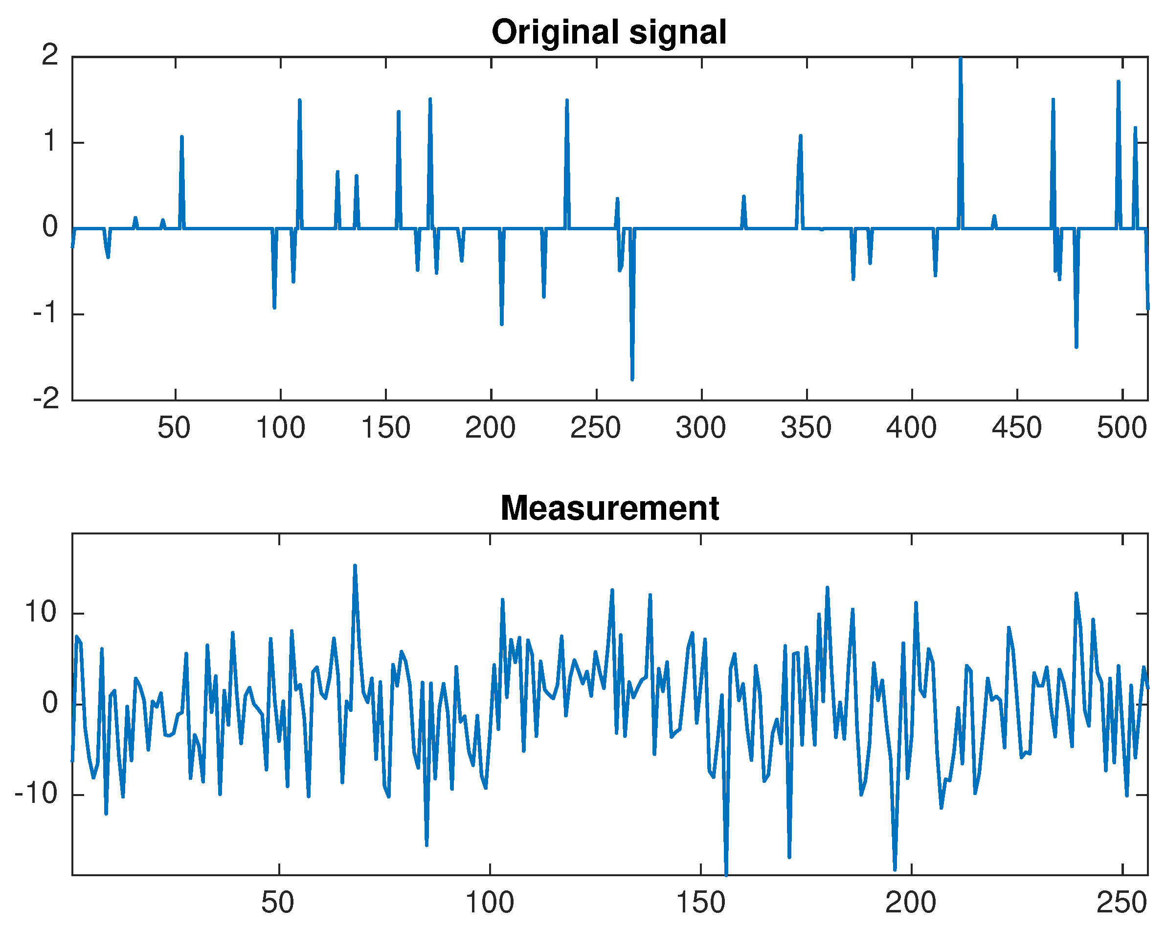
In this experiment, the size of signal is selected to be $N=512$, and $M=256$, where the original signal contains m nonzero elements. Let T be the Gaussian matrix generated by command $randn(M,N)$. Choose $S={\mathrm{prox}}_{\frac{1}{{\parallel T\parallel }^2}h}(I-\frac{1}{{\parallel T\parallel }^2}\nabla g)$ and $f(·)=\frac{1}{10}(·)$. Assume the same ${\alpha }_n$, ${\beta }_n$, $\mu$, and ${\lambda }_1$ as in the preceding example. Given that the initial point $x_1$ is chosen to be $T^{t}b$, use the mean-squared error to measure the restoration accuracy. Precisely, $MS{E}_n=\frac{1}{N}{\parallel x_n-x\parallel }^2<5\times {10}^{-5}$, where x is the original signal. Then the results are displayed in Table 2. In other words, the number of iterations and elapsed time of each algorithm are provided for different numbers of nonzero elements. The numerical results show that our algorithm has a better elapsed time and number of iterations than Algorithm 3.1 [6].

Table 2. Numerical comparison between Algorithm 3.1 [6] and the new algorithm for $\sigma =0.01$.

m Nonzero Elements	Algorithm 3.1 [6]		New Algorithm
	Elapsed Time (s)	No. of Iter.	Elapsed Time (s)	No. of Iter.
$m=8$	0.3263	1703	0.1293	688
$m=16$	0.4655	3331	0.1985	1285
$m=24$	0.5966	4607	0.2990	1777
$m=32$	0.6644	4778	0.3321	1808
$m=40$	0.7323	5644	0.4051	2144

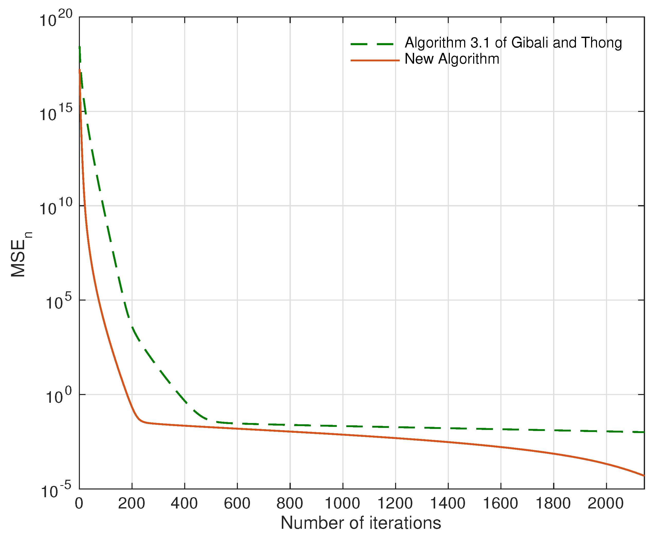
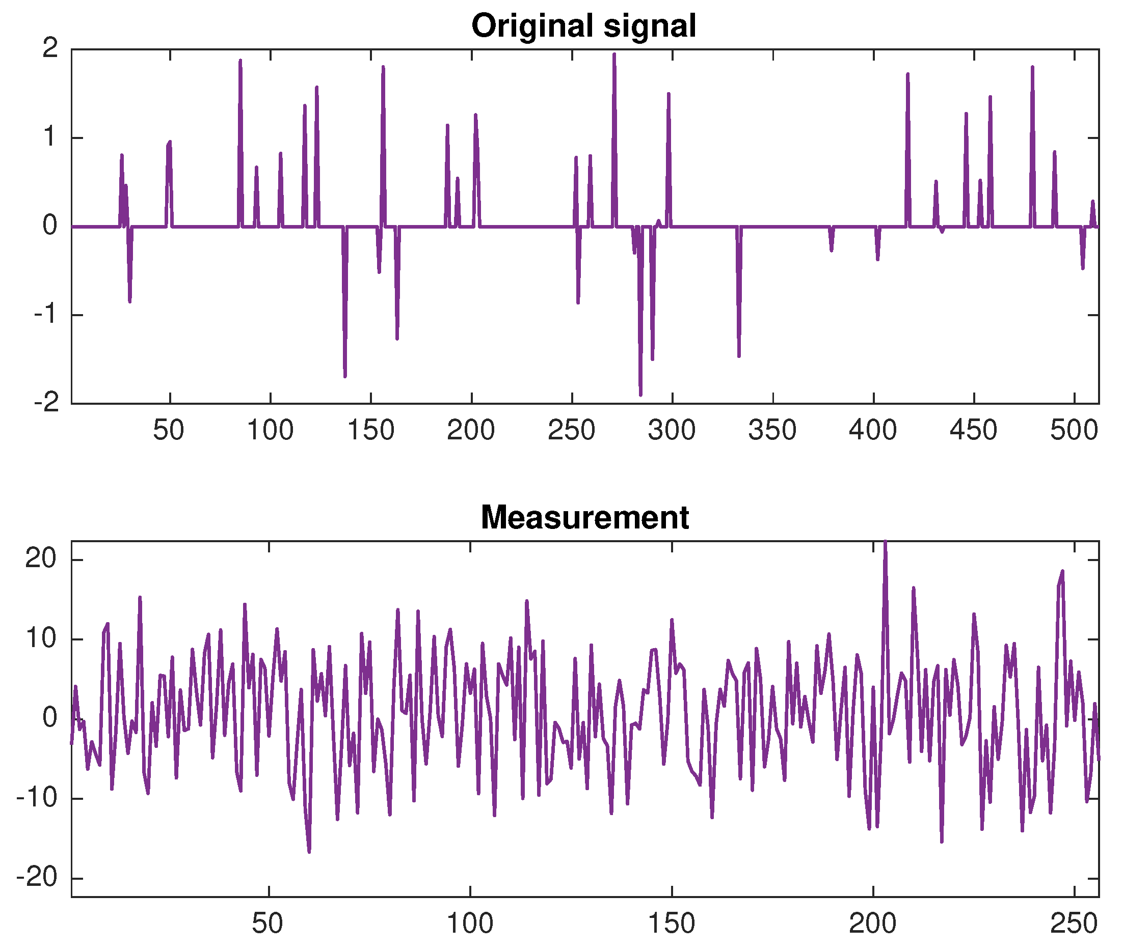
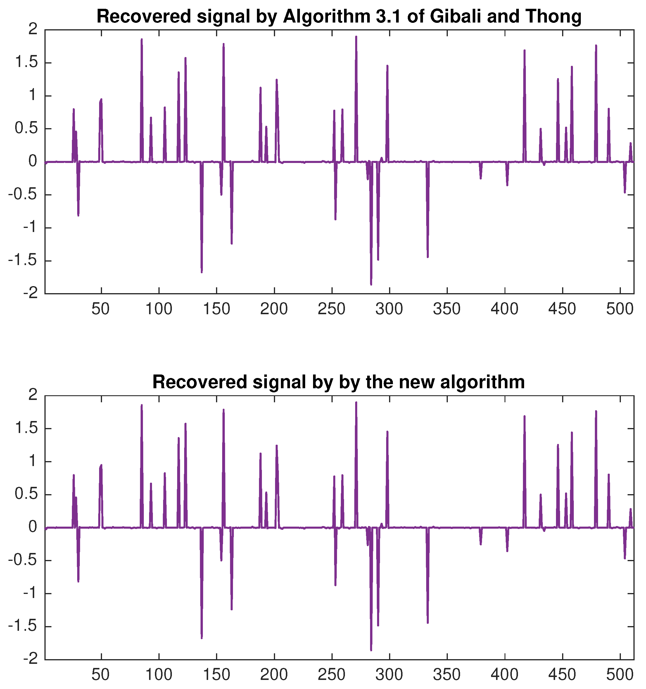
On top of that, we compare the recovery signals of each algorithm. In Figure 1, the original signal and the measurement are shown in the case when $m=40$ and $\sigma =0.01$. Then the signals recovered by using Algorithm 3.1 [6] and the new algorithm are presented in Figure 2. Therefore, the errors of each algorithm are compared in Figure 3. The outcome is that the signal recovered from our algorithm contains less error than Algorithm 3.1 [6].

Figure 1. The original signal and the measurement when $m=40$ and $\sigma =0.01$.

Figure 2. The recovery signals by Algorithm 3.1 [6] and the new algorithm when $m=40$ and $\sigma =0.01$.

Figure 3. Error plotting of Algorithm 3.1 [6] and the new algorithm when $m=40$ and $\sigma =0.01$.

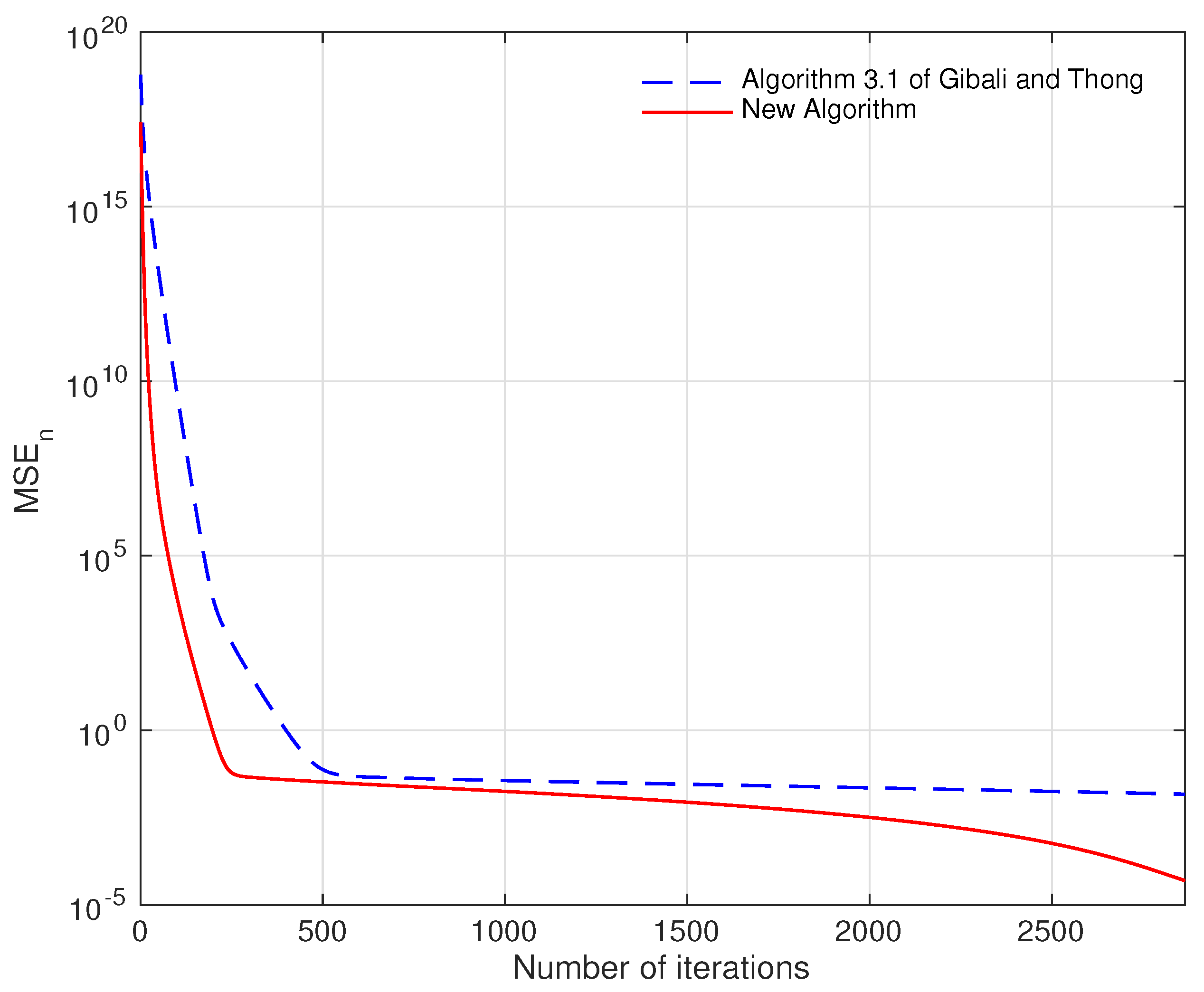
Next, another numerical result is given for $\sigma =0.1$ in Table 3. Likewise, the original signal and the measurement are shown when $m=40$ in Figure 4. By using Algorithm 3.1 [6] and the new algorithm, the signal is recovered as in Figure 5. Then Figure 6 shows that the error of the result obtained from our algorithm is less than the result obtained from Algorithm 3.1 [6].

Table 3. Numerical comparison between Algorithm 3.1 [6] and the new algorithm for $\sigma =0.1$.

m Nonzero Elements	Algorithm 3.1 [6]		New Algorithm
	Elapsed Time (s)	No. of Iter.	Elapsed Time (s)	No. of Iter.
$m=8$	0.3848	2059	0.1292	811
$m=16$	0.5229	3598	0.2583	1417
$m=24$	0.5954	4098	0.2927	1562
$m=32$	0.9350	5537	0.4221	2218
$m=40$	1.1025	7350	0.5007	2865

Figure 4. The original signal and the measurement when $m=40$ and $\sigma =0.1$.

Figure 5. The recovery signals by Algorithm 3.1 [6] and the new algorithm when $m=40$ and $\sigma =0.1$.

Figure 6. Error plotting of Algorithm 3.1 [6] and the new algorithm when $m=40$ and $\sigma =0.1$.

Overall, based on Table 2 and Table 3, similar results as in Example 1 is obtained. The new algorithm improves the elapsed time, and reduces the number of iterations compared to Algorithm 3.1 [6]. This means that the new algorithm displays better results than Algorithm 3.1 [6], mainly because of the more general setting in the new algorithm.

5. Conclusions

To sum up, a modified Tseng type algorithm is created based on the methods of Mann iterations and viscosity approximation. The purpose is to find a common solution to the inclusion problem of an L-Lipschitz continuous and monotone single-valued operator and a maximal monotone multivalued operator, and the fixed point problem of a nonexpansive operator. With some extra conditions, the iteration defined by the algorithm converges strongly to the solution of the problem. In applications, this algorithm can be applied to the convex feasibility problem and the signal recovery in compressed sensing. The numerical experiments of our algorithm yield better results compared to the previous algorithm.

References

- Censor, Y.; Bortfeld, T.; Martin, B.; Trofimov, A. A unified approach for inversion problems in intensity-modulated radiation therapy. Phys. Med. Biol. 2006, 51, 2353–2365. [Google Scholar] [CrossRef] [PubMed]
- Censor, Y.; Elfving, T. A multiprojection algorithm using Bregman projections in a product space. Numer. Algorithms 1994, 8, 221–239. [Google Scholar] [CrossRef]
- Cholamjiak, P.; Shehu, Y. Inertial forward–backward splitting method in Banach spaces with application to compressed sensing. Appl. Math. 2019, 64, 409–435. [Google Scholar] [CrossRef]
- Combettes, P.L.; Wajs, V.R. Signal recovery by proximal forward–backward splitting. Multiscale Model. Simul. 2005, 4, 1168–1200. [Google Scholar] [CrossRef]
- Duchi, J.; Shalev-Shwartz, S.; Singer, Y.; Chandra, T. Efficient projections onto the l1-ball for learning in high dimensions. In Proceedings of the 25th International Conference on Machine Learning, Helsinki, Finland, 5–8 July 2008. [Google Scholar]
- Gibali, A.; Thong, D.V. Tseng type methods for solving inclusion problems and its applications. Calcolo 2018, 55, 49. [Google Scholar] [CrossRef]
- Kitkuan, D.; Kumam, P.; Martínez-Moreno, J.; Sitthithakerngkiet, K. Inertial viscosity forward–backward splitting algorithm for monotone inclusions and its application to image restoration problems. Int. J. Comput. Math. 2019, 1–19. [Google Scholar] [CrossRef]
- Suparatulatorn, R.; Khemphet, A.; Charoensawan, P.; Suantai, S.; Phudolsitthiphat, N. Generalized self-adaptive algorithm for solving split common fixed point problem and its application to image restoration problem. Int. J. Comput. Math. 2019, 1–15. [Google Scholar] [CrossRef]
- Suparatulatorn, R.; Charoensawan, P.; Poochinapan, K. Inertial self-adaptive algorithm for solving split feasible problems with applications to image restoration. Math. Methods Appl. Sci. 2019, 42, 7268–7284. [Google Scholar] [CrossRef]
- Attouch, H.; Peypouquet, J.; Redont, P. Backward-forward algorithms for structured monotone inclusions in Hilbert spaces. J. Math. Anal. Appl. 2018, 457, 1095–1117. [Google Scholar] [CrossRef]
- Dong, Y.D.; Fischer, A. A family of operator splitting methods revisited. Nonlinear Anal. 2010, 72, 4307–4315. [Google Scholar] [CrossRef]
- Huang, Y.Y.; Dong, Y.D. New properties of forward–backward splitting and a practical proximal-descent algorithm. Appl. Math. Comput. 2014, 237, 60–68. [Google Scholar] [CrossRef]
- Rockafellar, R.T. Monotone operators and the proximal point algorithm. SIAM J. Control Optim. 1976, 14, 877–898. [Google Scholar] [CrossRef]
- Lions, P.L.; Mercier, B. Splitting algorithms for the sum of two nonlinear operators. SIAM J. Numer. Anal. 1979, 16, 964–979. [Google Scholar] [CrossRef]
- Passty, G.B. Ergodic convergence to a zero of the sum of monotone operators in Hilbert space. J. Math. Anal. Appl. 1979, 72, 383–390. [Google Scholar] [CrossRef]
- Chen, H.G.; Rockafellar, R.T. Convergence rates in forward–backward splitting. SIAM J. Optim. 1997, 7, 421–444. [Google Scholar] [CrossRef]
- Tseng, P. A modified forward–backward splitting method for maximal monotone mappings. SIAM J. Control Optim. 2000, 38, 431–446. [Google Scholar] [CrossRef]
- Zhang, J.; Jiang, N. Hybrid algorithm for common solution of monotone inclusion problem and fixed point problem and application to variational inequalities. SpringerPlus 2016, 5, 803. [Google Scholar] [CrossRef][Green Version]
- Thong, D.V.; Vinh, N.T. Inertial methods for fixed point problems and zero point problems of the sum of two monotone mappings. Optimization 2019, 68, 1037–1072. [Google Scholar] [CrossRef]
- Cholamjiak, P.; Kesornprom, S.; Pholasa, N. Weak and strong convergence theorems for the inclusion problem and the fixed-point problem of nonexpansive mappings. Mathematics 2019, 7, 167. [Google Scholar] [CrossRef]
- Brézis, H.; Chapitre, I.I. Operateurs maximaux monotones. North-Holland Math. Stud. 1973, 5, 19–51. [Google Scholar]
- Goebel, K.; Kirk, W.A. Topics in Metric Fixed Point Theory; Cambridge University Press: Cambridge, UK, 1990. [Google Scholar]
- Xu, H.K. Iterative algorithms for nonlinear operators. J. Lond. Math. Soc. 2002, 66, 240–256. [Google Scholar] [CrossRef]
- Maingé, P.E. Strong convergence of projected subgradient methods for nonsmooth and non- strictly convex minimization. Set-Valued Anal. 2008, 16, 899–912. [Google Scholar] [CrossRef]
- Mann, W.R. Mean value methods in iteration. Proc. Am. Math. Soc. 1953, 4, 506–510. [Google Scholar] [CrossRef]
- Moudafi, A. Viscosity approximating methods for fixed point problems. J. Math. Anal. Appl. 2000, 241, 46–55. [Google Scholar] [CrossRef]
- Bauschke, H.H.; Combettes, P.L. Convex Analysis and Monotone Operator Theory in Hilbert Spaces; CMS Books in Mathematics; Springer: New York, NY, USA, 2011. [Google Scholar]
- Iiduka, H.; Takahashi, W. Strong convergence theorems for nonexpansive nonself-mappings and inverse-strongly-monotone mappings. J. Convex Anal. 2004, 11, 69–79. [Google Scholar]
© 2019 by the authors. Licensee MDPI, Basel, Switzerland. This article is an open access article distributed under the terms and conditions of the Creative Commons Attribution (CC BY) license (http://creativecommons.org/licenses/by/4.0/).