Some Novel Interactive Hybrid Weighted Aggregation Operators with Pythagorean Fuzzy Numbers and Their Applications to Decision Making

Abstract

A Pythagorean fuzzy set (PFS) is one of the extensions of the intuitionistic fuzzy set which accommodate more uncertainties to depict the fuzzy information and hence its applications are more extensive. In the modern decision-making process, aggregation operators are regarded as a useful tool for assessing the given alternatives and whose target is to integrate all the given individual evaluation values into a collective one. Motivated by these primary characteristics, the aim of the present work is to explore a group of interactive hybrid weighted aggregation operators for assembling Pythagorean fuzzy sets to deal with the decision information. The proposed aggregation operators include interactive the hybrid weighted average, interactive hybrid weighted geometric and its generalized versions. The major advantages of the proposed operators to address the decision-making problems are (i) to consider the interaction among membership and non-membership grades of the Pythagorean fuzzy numbers, (ii) it has the property of idempotency and simple computation process, and (iii) it possess an adjust parameter value and can reflect the preference of decision-makers during the decision process. Furthermore, we introduce an innovative multiple attribute decision making (MADM) process under the PFS environment based on suggested operators and illustrate with numerous numerical cases to verify it. The comparative analysis as well as advantages of the proposed framework confirms the supremacies of the method.

1. Introduction

Multiple attribute decision making (MADM) is one of the processes to find the most desirable alternative among all given alternatives in the light of finite attributes or criteria. In the decision-making process, it is commonly supposed that the evaluation information of alternatives for attributes described by decision-makers (DMs) is precise numbers. However, due to the indeterminacy of the practical environment and human cognition, DMs are usually do not find it easy to use crisp numbers to express their preferences. An appropriate way to deal with such problems is to adopt uncertain evaluations rather than crisp ones, for instance, an intuitionistic fuzzy set (IFS) [1] and fuzzy set (FS) [2]. As a successful extension of the notions of IFS and FS, the Pythagorean fuzzy set (PFS) was put forward by Yager [3,4]. Similar to the IFS, the PFS is still depicted by the membership and non-membership degrees, but their square sum within interval (0, 1). Thus, PFS is more versatile than IFS. For instance, if the membership grade is given as 0.4 by DM, while the non-membership grade is 0.8, it can be seen that $0.4+0.8>1$, so IFS cannot solve this issue, but since ${0.4}^2+{0.8}^2<1$, then the PFS can easily deal with it. Therefore, in some cases, the PFS can settle a large number of problems, while the IFS cannot. Since PFS appeared, it has become a useful technique for modeling vagueness and indeterminacy of the MADM issues or multiple attribute group decision making (MAGDM) issues [5,6,7,8,9,10,11,12]. Some evaluation methods in the light of PFS are given to solve Pythagorean fuzzy MADM problems. For instance, Rani et al. [13] extended traditional TOPSIS (technique for an order of preference by similarity to ideal solution) approach to Pythagorean fuzzy numbers (PFNs) and studied the selection of a sustainable recycling partner. Considering DM’s psychological characteristics, in the light of the prospect and regret theories, Peng and Dai [14] explored a stochastic decision approach under Pythagorean fuzzy setting. Ren et al. [15] extended traditional TODIM (an acronym in Portuguese of interactive and multiple attribute decision making) approach to PFNs. Chen [16] introduced a Pythagorean fuzzy VIKOR (vlseKriterijumska optimizacija I Kompromisno Resenje in Serbian) approach for MADM. Zhang [17] expanded the hierarchical QUALIFLEX (qualitative flexible multiple criteria method) algorithm to the interval-valued PFSs, and employed it to investigate the industries’ risk evaluation.

The way of evaluation methods in Pythagorean fuzzy decision-making problems is only one aspect, the other significant aspect is to aggregate these evaluation values. Aggregation operators (AOs) can integrate all the given individual evaluation values into a collective one, which is regarded as a useful tool for assessing alternatives. Now AOs are investigated more broadly under the Pythagorean fuzzy environment, and the research related to AOs are from general categories:

(1)

The operation of AOs defined by classical operational rules with PFSs [12]. Wei and Lu [18] developed six power AOs in Pythagorean fuzzy setting and also discussed desirable properties of them. Ma and Xu [19] employed the symmetric Pythagorean fuzzy AOs to settle MADM problems. Garg [20,21] defined exponential operation and logarithms operations for PFSs and discussed their relevant aggregation operators. In the light of the Einstein t-norm operations, Garg [22,23] introduced a series of generalized Pythagorean averaging and geometric AOs. With the aid of the Hamacher operations, Wu and Wei [24] introduced several Hamacher AOs for managing Pythagorean fuzzy MADM problems. Yu et al. [25] presented a kind of new Pythagorean fuzzy distance AOs. Wang and Li [26] developed four continuous interval-valued Pythagorean fuzzy AOs in MAGDM. Taking the relationship of aggregated PFNs into account, Qin [27] introduced the generalized form of Pythagorean fuzzy Maclaurin symmetric means. With the aid of the traditional Bonferroni mean (BM), Liang et al. [28] discussed a Pythagorean fuzzy geometric BM (PFGBM) operator. After that, a partitioned PFGBM operator was introduced by Liang et al. [29]. Wei and Lu [30] defined the Pythagorean fuzzy Maclaurin symmetric mean AOs for PFNs. Li et al. [31] proposed a series of Hamy mean operators under a Pythagorean fuzzy context. Li et al. [32] investigated two Pythagorean fuzzy power Muirhead mean AOs along with their properties and applied them to deal with the evaluation of domestic airlines.

(2)

The operation of AOs defined by the interactive operational rules with PFSs [33]. It is more reasonable in some situations, because it captures the interactive influence over the membership and non-membership grades of PFNs. For example, Let ${\alpha }_1=({\mu }_{{\alpha }_1},{\nu }_{{\alpha }_1})$ and ${\alpha }_2=({\mu }_{{\alpha }_2},{\nu }_{{\alpha }_2})$ be two PFNs, if membership degrees ${\mu }_{{\alpha }_1}=0$ and ${\mu }_{{\alpha }_2}\ne 0$, then in the light of operational rules [12], we get membership degree ${\mu }_{{\alpha }_1\oplus {\alpha }_2}=0$, which implies that ${\mu }_{{\alpha }_2}$ has no effect on the result ${\mu }_{{\alpha }_1\oplus {\alpha }_2}$. Similarly, if non-membership degrees ${\nu }_{{\alpha }_1}=0$ and ${\nu }_{{\alpha }_2}\ne 0$, then ${\nu }_{{\alpha }_2}$ has no effect on the result non-membership degree ${\nu }_{{\alpha }_1\otimes {\alpha }_2}$. To overcome this issue, Wei [33] introduced the interactive operation for PFNs and also some corresponding interactive AOs were developed. They are Pythagorean fuzzy interactive weighted average (PFIWA), ordered weighted average (PFIOWA), hybrid average (PFIHA), weighted geometric (PFIWG), ordered weighted geometric (PFIOWG) and hybrid geometric (PFIHG) operators. Garg [34,35] presented the concept of neutrality operational laws for PFNs and the AOs for solving the group decision making problems. Gao et al. [36] defined some interactive power AOs for PFNs. Yang and Pang [37] presented interactive Maclaurin symmetric mean AOs and corresponding weighted forms using the different PFNs for dealing with MADM problems. Garg [38] presented the generalized interactive weighted Einstein AOs for PFNs and hence solved the decision-making problems. Yang et al. [39] extended the traditional BM operator to a Pythagorean fuzzy environment and proposed some interactive partitioned BM operators as well as their interesting properties.

From these above analyses, we can see that different aggregation operators have different features and application aspects. The PFIWA and the PFIWG AOs can weigh only the significance of PFNs themselves, while the PFIOWA and the PFIOWG AOs can weigh the ordered positions of given PFNs but cannot weigh the PFNs themselves. Moreover, the PFIHA and the PFIHG operators may weigh all aggregated PFNs and correspond ordered positions of them. Therefore, the PFIHA and the PFIHG operators have some superiority over the operators described above. However, these two operators have a drawback that the aggregated value of some identical integrated PFNs relies on the weight values, that is they do not possess the property of idempotency. It was pointed out by Liao and Xu [40], hybrid aggregation operators should satisfy the basic property of idempotency, so they presented a group of hybrid operators under a hesitant fuzzy environment. However, these aggregation operators are not available to tackle the Pythagorean fuzzy MADM problems. PFS, a valuable generalization of IFSs, has been shown as a successful means to deal with the indeterminacy and fuzziness which appear in many real decision problems. The presented research concentrated on the Pythagorean fuzzy setting. Therefore, it was worth putting forward some novel Pythagorean fuzzy interactive hybrid operators. Inspired by this idea, the motivation and objective of this manuscript were to

(1)

explore novel Pythagorean fuzzy interactive hybrid weighted average (PFIHWA) and geometric (PFIHWG) operators, discuss some interesting properties and particular cases;

(2)

propose novel generalized PFIHWA (GPFIHWA) and generalized PFIHWG (GPFIHWG) operators, also study their desirable properties and special cases;

(3)

introduce some steps for MADM and MAGDM by using the proposed operators;

(4)

demonstrate the availability and flexibility of the proposed MADM and MAGDM methods through some practical examples.

The remaining paper is arranged as follows: Some fundamental notions about PFSs and the AOs are introduced in Section 2. Novel PFIHWA and PFIHWG operators along with their properties are given in Section 3. Generalized forms of the AOs are provided in Section 4. In Section 5, we use the presented AOs to tackle the MADM problems and MAGDM problems, and the availability as well as flexibility of the proposed methods is illustrated with some real examples. Section 6 summarizes the paper.

2. Preliminaries

We briefly review some fundamental notions about PFS and Pythagorean fuzzy AOs in this part.

2.1. Pythagorean Fuzzy Sets

Definition 1

[12]. Let $Y$ be a universal set, a PFS $P$ is defined as:

$$P=\left\{\langle y,\left({\mu }_P(y),{\nu }_P(y)\right)\rangle |y\in Y\right\},$$

(1)

where ${\mu }_P(y),{\nu }_P(y)\in [0,1]$ meet the condition: ${\left({\mu }_P(y)\right)}^2+{\left({\nu }_P(y)\right)}^2\in [0,1]$. ${\mu }_P(y),v_P(y)$ define degrees of membership and non-membership for every $y\in Y$, respectively. Indeterminacy degree is ${\pi }_P(y)=\sqrt{1-{\left({\mu }_P(y)\right)}^2-{\left({\nu }_P(y)\right)}^2}$.

Zhang and Xu [12] called $\alpha =(\mu ,\nu )$ as a PFN, meets the condition $\mu \in [0,1],\nu \in [0,1]$ and ${\mu }_{}^2+{\nu }_{}^2\in [0,1]$. $\Omega$ denotes all Pythagorean fuzzy numbers (PFNs).

Some fundamental operational rules for PFNs given by Zhang and Xu [12] as follows:

Definition 2

[12]. Let $\alpha =(\mu ,\nu ),{\alpha }_1=({\mu }_1,{\nu }_1)$ and ${\alpha }_2=({\mu }_2,{\nu }_2)$ be three PFNs, then their operational laws are shown as follows:

$$\begin{array}{l}(1){\alpha }^c=(\nu ,\mu );\\ (2){\alpha }_1\oplus {\alpha }_2=\left(\sqrt{{({\mu }_1)}^2+{({\mu }_2)}^2-{({\mu }_1)}^2{({\mu }_2)}^2},{\nu }_1{\nu }_2\right);\\ (3){\alpha }_1\otimes {\alpha }_2=\left({\mu }_1{\mu }_2,\sqrt{{({\nu }_1)}^2+{({\nu }_2)}^2-{({\nu }_1)}^2{({\nu }_2)}^2}\right);\\ (4)\lambda \alpha =\left(\sqrt{1-{(1-{\mu }^2)}^{\lambda }},{\nu }^{\lambda }\right),\lambda >0;\\ (5){\alpha }^{\lambda }=\left({\mu }^{\lambda },\sqrt{1-{(1-{\nu }^2)}^{\lambda }}\right),\lambda >0,\end{array}$$

where ${\alpha }^c$ denotes complement operation of $\alpha$. $\oplus$ and $\otimes$ denote addition and multiplication between ${\alpha }_1$ and ${\alpha }_2$, respectively.

Definition 3

[33]. Let $\alpha =(\mu ,\nu ),{\alpha }_1=({\mu }_1,{\nu }_1)$ and ${\alpha }_2=({\mu }_2,{\nu }_2)$ be three PFNs, then the interactive operational laws are given as follows:

$$\begin{array}{l}(1){\alpha }_1\oplus {\alpha }_2=\left(\sqrt{{({\mu }_1)}^2+{({\mu }_2)}^2-{({\mu }_1)}^2{({\mu }_2)}^2},\sqrt{{({\nu }_1)}^2+{({\nu }_2)}^2-{({\nu }_1)}^2{({\nu }_2)}^2-{({\mu }_1)}^2{({\nu }_2)}^2-{({\nu }_1)}^2{({\mu }_2)}^2}\right);\\ (2){\alpha }_1\otimes {\alpha }_2=\left(\sqrt{{({\mu }_1)}^2+{({\mu }_2)}^2-{({\mu }_1)}^2{({\mu }_2)}^2-{({\mu }_1)}^2{({\nu }_2)}^2-{({\nu }_1)}^2{({\mu }_2)}^2},\sqrt{{({\nu }_1)}^2+{({\nu }_2)}^2-{({\nu }_1)}^2{({\nu }_2)}^2}\right);\\ (3)\lambda \alpha =\left(\sqrt{1-{(1-{\mu }^2)}^{\lambda }},\sqrt{{(1-{\mu }^2)}^{\lambda }-{(1-({\mu }^2+{\nu }^2))}^{\lambda }}\right),\lambda >0;\\ (4){\alpha }^{\lambda }=\left(\sqrt{{(1-{\nu }^2)}^{\lambda }-{(1-({\mu }^2+{\nu }^2))}^{\lambda }},\sqrt{1-{(1-{\nu }^2)}^{\lambda }}\right),\lambda >0.\end{array}$$

Definition 4

[12]. Let $\alpha =(\mu ,\nu )$ be a PFN, $s(\alpha )={\mu }_{}^2-{\nu }_{}^2$ and $a(\alpha )={\mu }_{}^2+{\nu }_{}^2$ denote the score and the accuracy degree of $\alpha$, respectively. For two PFNs ${\beta }_1,{\beta }_2$, we have

(1)

If$s({\beta }_1)>s({\beta }_2)$, then${\beta }_1\succ {\beta }_2$;

(2)

If$s({\beta }_1)=s({\beta }_2)$, then:

(a)

If$a({\beta }_1)>a({\beta }_2)$, then${\beta }_1\succ {\beta }_2$;

(b)

If$a({\beta }_1)=a({\beta }_2)$, then${\beta }_1={\beta }_2$.

2.2. Interactive Aggregation Operators for PFNs

With the aid of interactive operational rules given as Definition 3, Wei [33] proposed some interactive aggregation operators for PFNs:

Definition 5

[33]. Suppose that ${\alpha }_j=({\mu }_j,{\nu }_j)(j=1,2,3,\dots ,n)$ are a family of PFNs and $\omega ={({\omega }_1,{\omega }_2,\dots ,{\omega }_n)}^T$ is the collection relevant vector of ${\alpha }_j$, with ${\omega }_j\ge 0$, ${\displaystyle {\sum }_{j=1}^n{\omega }_j=1}$. Then

(1) A PFIWA operator is a function$\mathrm{PFIWA}:{\Omega }^n\to \Omega$, and

$$\begin{array}{l}\mathrm{PFIWA}({\alpha }_1,{\alpha }_2,\dots ,{\alpha }_n)=\\ {\displaystyle \underset{j=1}{\overset{n}{\oplus }}}{\omega }_j{\alpha }_j=\left(\sqrt{1-{\displaystyle {\displaystyle \prod }_{j=1}^n}{\left(1-{({\mu }_j)}^2\right)}^{{\omega }_j}},\sqrt{{\displaystyle {\displaystyle \prod }_{j=1}^n}{\left(1-{({\mu }_j)}^2\right)}^{{\omega }_j}-{\displaystyle {\displaystyle \prod }_{j=1}^n}{\left(1-\left({({\mu }_j)}^2+{({\nu }_j)}^2\right)\right)}^{{\omega }_j}}\right)\end{array}$$

(2)

(2) A PFIWG operator is a function$\mathrm{PFIWG}:{\Omega }^n\to \Omega$, and

$$\begin{array}{l}\mathrm{PFIWG}({\alpha }_1,{\alpha }_2,\dots ,{\alpha }_n)=\\ {\displaystyle \underset{j=1}{\overset{n}{\otimes }}}{\left({\alpha }_j\right)}^{{\omega }_j}=\left(\sqrt{{\displaystyle {\displaystyle \prod }_{j=1}^n}{\left(1-{({\nu }_j)}^2\right)}^{{\omega }_j}-{\displaystyle {\displaystyle \prod }_{j=1}^n}{\left(1-\left({({\mu }_j)}^2+{({\nu }_j)}^2\right)\right)}^{{\omega }_j}},\sqrt{1-{\displaystyle {\displaystyle \prod }_{j=1}^n}{\left(1-{({\nu }_j)}^2\right)}^{{\omega }_j}}\right)\end{array}$$

(3)

Definition 6

[33]. Suppose that ${\alpha }_j=({\mu }_j,{\nu }_j)(j=1,2,3,\dots ,n)$ are a family of PFNs and $\omega ={({\omega }_1,{\omega }_2,\dots ,{\omega }_n)}^T$ is the collection relevant vector of ${\alpha }_j$, with ${\omega }_j\ge 0$, ${\displaystyle {\sum }_{j=1}^n{\omega }_j=1}$. $((1),(2),(3)\dots ,(n))$ means any permutation of $(1,2,3,\cdots ,n)$ satisfies ${\alpha }_{(j-1)}\ge {\alpha }_{(j)}$. Then

(1) A PFIOWA operator is a function$\mathrm{PFIOWA}:{\Omega }^n\to \Omega$, and

$$\begin{array}{l}\mathrm{PFIOWA}({\alpha }_1,{\alpha }_2,\dots ,{\alpha }_n)=\\ {\displaystyle \underset{j=1}{\overset{n}{\oplus }}}{\omega }_j{\alpha }_{(j)}=\left(\sqrt{1-{\displaystyle {\displaystyle \prod }_{j=1}^n}{\left(1-{({\mu }_{(j)})}^2\right)}^{{\omega }_j}},\sqrt{{\displaystyle {\displaystyle \prod }_{j=1}^n}{\left(1-{({\mu }_{(j)})}^2\right)}^{{\omega }_j}-{\displaystyle {\displaystyle \prod }_{j=1}^n}{\left(1-\left({({\mu }_{(j)})}^2+{({\nu }_{(j)})}^2\right)\right)}^{{\omega }_j}}\right).\end{array}$$

(4)

(2) A PFIOWG operator is a function$\mathrm{PFIOWG}:{\Omega }^n\to \Omega$, and

$$\begin{array}{l}\mathrm{PFIOWG}({\alpha }_1,{\alpha }_2,\dots ,{\alpha }_n)=\\ {\displaystyle \underset{j=1}{\overset{n}{\otimes }}}{\left({\alpha }_{(j)}\right)}^{{\omega }_j}=\left(\sqrt{{\displaystyle {\displaystyle \prod }_{j=1}^n}{\left(1-{({\nu }_{(j)})}^2\right)}^{{\omega }_j}-{\displaystyle {\displaystyle \prod }_{j=1}^n}{\left(1-\left({({\mu }_{(j)})}^2+{({\nu }_{(j)})}^2\right)\right)}^{{\omega }_j}},\sqrt{1-{\displaystyle {\displaystyle \prod }_{j=1}^n}{\left(1-{({\nu }_{(j)})}^2\right)}^{{\omega }_j}}\right)\end{array}$$

(5)

Especially, if$\omega =(\frac{1}{n},\frac{1}{n},\dots ,\frac{1}{n})$, then the PFIOWA (PFIOWG)operator becomes the PFIWA(PFIWG) operator.

Definition 7

[33]. Suppose that ${\alpha }_j=({\mu }_j,{\nu }_j)(j=1,2,3,\dots ,n)$ are a family of PFNs and $\omega ={({\omega }_1,{\omega }_2,\dots ,{\omega }_n)}^T$ is the collection relevant vector of ${\alpha }_j$, with ${\omega }_j\ge 0$, ${\displaystyle {\sum }_{j=1}^n{\omega }_j=1}$. $((1),(2),(3)\dots ,(n))$ means any permutation of $(1,2,3,\cdots ,n)$ satisfies ${\alpha }_{(j-1)}\ge {\alpha }_{(j)}$.$\epsilon ={({\epsilon }_1,{\epsilon }_2,\dots ,{\epsilon }_n)}^T$ denotes the weight vector of ${\alpha }_j$ $(j=1,2,\dots ,n)$ with ${\epsilon }_j\ge 0$, ${\displaystyle {\sum }_{j=1}^n{\epsilon }_j=1}$. Thus

(1) A PFIHA operator is a function$\mathrm{PFIHA}:{\Omega }^n\to \Omega$, and

$$\begin{array}{l}\mathrm{PFIHA}({\alpha }_1,{\alpha }_2,\dots ,{\alpha }_n)=\\ {\displaystyle \underset{j=1}{\overset{n}{\oplus }}}{\omega }_j{\dot{\alpha }}_{(j)}=\left(\sqrt{1-{\displaystyle {\displaystyle \prod }_{j=1}^n}{\left(1-{({\dot{\mu }}_{(j)})}^2\right)}^{{\omega }_j}},\sqrt{{\displaystyle {\displaystyle \prod }_{j=1}^n}{\left(1-{({\dot{\mu }}_{(j)})}^2\right)}^{{\omega }_j}-{\displaystyle {\displaystyle \prod }_{j=1}^n}{\left(1-\left({({\dot{\mu }}_{(j)})}^2+{({\dot{\nu }}_{(j)})}^2\right)\right)}^{{\omega }_j}}\right)\end{array}$$

(6)

in which,${\dot{\alpha }}_{(j)}$is the$j$-th largest value of weighted PFNs$\{n{\epsilon }_1{\alpha }_1,n{\epsilon }_2{\alpha }_2,\cdots ,n{\epsilon }_n{\alpha }_n\}$,$n$indicates the balancing coefficient.

(2) A PFIHG operator is a function$\mathrm{PFIHG}:{\Omega }^n\to \Omega$, and

$$\begin{array}{l}\mathrm{PFIHG}({\alpha }_1,{\alpha }_2,\dots ,{\alpha }_n)=\\ {\displaystyle \underset{j=1}{\overset{n}{\otimes }}}{\left({\dot{\alpha }}_{(j)}\right)}^{{\omega }_j}=\left(\sqrt{{\displaystyle {\displaystyle \prod }_{j=1}^n}{\left(1-{({\dot{\nu }}_{(j)})}^2\right)}^{{\omega }_j}-{\displaystyle {\displaystyle \prod }_{j=1}^n}{\left(1-\left({({\dot{\mu }}_{(j)})}^2+{({\dot{\nu }}_{(j)})}^2\right)\right)}^{{\omega }_j}},\sqrt{1-{\displaystyle {\displaystyle \prod }_{j=1}^n}{\left(1-{({\dot{\nu }}_{(j)})}^2\right)}^{{\omega }_j}}\right)\end{array}$$

(7)

in which,${\dot{\alpha }}_{(j)}$is the$j$-th largest value of weighted PFNs$\{{({\alpha }_1)}^{n{\epsilon }_1},{({\alpha }_2)}^{n{\epsilon }_2},\cdots ,{({\alpha }_n)}^{n{\epsilon }_n}\}$,$n$indicates the balancing coefficient.

Especially, if$\omega =(\frac{1}{n},\frac{1}{n},\dots ,\frac{1}{n})$, then the PFIHA (PFIHG)operator becomes the PFIWA (PFIWG)operator. If$\epsilon =(\frac{1}{n},\frac{1}{n},\dots ,\frac{1}{n})$, then the PFIHA(PFIHG)operator becomes the PFIOWA (PFIOWG) operator.

3. Some Novel Pythagorean Fuzzy Interactive Hybrid Weighted Aggregation Operators

Although PFIHA (PFIHG) possesses both the advantages of the PFIWA (PFIWG) operator and the PFIOWA (PFIOWG) operator, have a shortcoming which is that the AOs do not meet the prominent property, that is idempotency.

3.1. Shortcoming of the Existing Operators

In the below example, we illustrate with a numerical example that the existing aggregation operators do not own the feature of the idempotency.

Example 1.

Let${\alpha }_1=(0.6,0.5)$,${\alpha }_2=(0.6,0.5)$,${\alpha }_3=(0.6,0.5)$be three PFNs, the corresponding weight vector is$\epsilon ={({\epsilon }_1,{\epsilon }_2,{\epsilon }_3)}^T={(0.7,0.2,0.1)}^T$. $\omega ={({\omega }_1,{\omega }_2,{\omega }_3)}^T={(0.3,0.5,0.2)}^T$is the aggregation associated vector. From Definition 3, we have

$$\begin{gathered} \begin{array}{l}{\dot{\alpha }}_1=n{\epsilon }_1{\alpha }_1=3\times 0.7\otimes (0.6,0.5)=2.1\otimes (0.6,0.5)\\ =\left(\sqrt{1-{(1-{0.6}^2)}^{2.1}},\sqrt{{(1-{0.6}^2)}^{2.1}-{(1-{0.6}^2-{0.5}^2)}^{2.1}}\right)=(0.7799,0.5033),\end{array} \\ \begin{array}{l}{\dot{\alpha }}_2=n{\epsilon }_2{\alpha }_2=3\times 0.2\otimes (0.6,0.5)=0.6\otimes (0.6,0.5)\\ =\left(\sqrt{1-{(1-{0.6}^2)}^{0.6}},\sqrt{{(1-{0.6}^2)}^{0.6}-{(1-{0.6}^2-{0.5}^2)}^{0.6}}\right)=(0.4847,0.4435),\end{array} \\ \begin{array}{l}{\dot{\alpha }}_3=n{\epsilon }_3{\alpha }_3=3\times 0.1\otimes (0.6,0.5)=0.3\otimes (0.6,0.5)\\ =\left(\sqrt{1-{(1-{0.6}^2)}^{0.3}},\sqrt{{(1-{0.6}^2)}^{0.3}-{(1-{0.6}^2-{0.5}^2)}^{0.3}}\right)=(0.3540,0.3475).\end{array} \end{gathered}$$

Based on Definition 4, we obtain$s({\dot{\alpha }}_1)=0.3549$,$s({\dot{\alpha }}_2)=0.0382$,$s({\dot{\alpha }}_3)=0.0046$, Since,$s({\dot{\alpha }}_1)>s({\dot{\alpha }}_2)>s({\dot{\alpha }}_3)$, then${\dot{\alpha }}_{(1)}={\dot{\alpha }}_1,{\dot{\alpha }}_{(2)}={\dot{\alpha }}_2,{\dot{\alpha }}_{(3)}={\dot{\alpha }}_3$. From Equation (6) in Definition 7, we obtain

$$\begin{array}{l}\mathrm{PFIHA}({\alpha }_1,{\alpha }_2,{\alpha }_3)={\displaystyle \underset{j=1}{\overset{3}{\oplus }}}{\omega }_j{\dot{\alpha }}_{(j)}=\\ \left(\begin{array}{l}\sqrt{1-{\left(1-{0.7799}^2\right)}^{0.3}{\left(1-{0.4847}^2\right)}^{0.5}{\left(1-{0.3540}^2\right)}^{0.2}},\\ \sqrt{\begin{array}{l}{\left(1-{0.7799}^2\right)}^{0.3}{\left(1-{0.4847}^2\right)}^{0.5}{\left(1-{0.3540}^2\right)}^{0.2}-{\left(1-{0.7799}^2-{0.5303}^2\right)}^{0.3}\\ {\left(1-{0.4847}^2-{0.4435}^2\right)}^{0.5}{\left(1-0.3540-{0.3475}^2\right)}^{0.2}\end{array}}\end{array}\right)\\ =(0.5976,0.4992)\ne (0.6,0.5).\end{array}$$

Similarly,

$$\begin{gathered} \begin{array}{l}{{\alpha }^{\prime }}_1={\left({\alpha }_1\right)}^{n{\epsilon }_1}={(0.6,0.5)}^{3\times 0.7}={(0.6,0.5)}^{2.1}=\\ \left(\sqrt{{(1-{0.5}^2)}^{2.1}-{(1-{0.6}^2-{0.5}^2)}^{2.1}},\sqrt{1-{(1-{0.5}^2)}^{2.1}},\right)=(0.6388,0.6734),\end{array} \\ \begin{array}{l}{{\alpha }^{\prime }}_2={\left({\alpha }_2\right)}^{n{\epsilon }_2}={(0.6,0.5)}^{3\times 0.2}={(0.6,0.5)}^{0.6}\\ =\left(\sqrt{{(1-{0.5}^2)}^{0.6}-{(1-{0.6}^2-{0.5}^2)}^{0.6}},\sqrt{1-{(1-{0.5}^2)}^{0.6}},\right)=(0.5226,0.3982),\end{array} \\ \begin{array}{l}{{\alpha }^{\prime }}_3={\left({\alpha }_3\right)}^{n{\epsilon }_3}={(0.6,0.5)}^{3\times 0.1}={(0.6,0.5)}^{0.3}\\ =\left(\sqrt{{(1-{0.5}^2)}^{0.3}-{(1-{0.6}^2-{0.5}^2)}^{0.3}},\sqrt{1-{(1-{0.5}^2)}^{0.3}},\right)=(0.4042,0.2876).\end{array} \end{gathered}$$

Based on Definition 4, we have$s({{\alpha }^{\prime }}_1)=-0.0454$,$s({{\alpha }^{\prime }}_2)=0.1145$,$s({{\alpha }^{\prime }}_3)=0.0807$, since,$s({{\alpha }^{\prime }}_2)>s({{\alpha }^{\prime }}_3)>s({{\alpha }^{\prime }}_1)$, then${{\alpha }^{\prime }}_{(1)}={{\alpha }^{\prime }}_2,{{\alpha }^{\prime }}_{(2)}={{\alpha }^{\prime }}_3,{{\alpha }^{\prime }}_{(3)}={{\alpha }^{\prime }}_1$. From Equation (7) in Definition 7, we obtain

$$\mathrm{PFIHG}({\alpha }_1,{\alpha }_2,{\alpha }_3)={\displaystyle \underset{j=1}{\overset{3}{\otimes }}}{\left({{\alpha }^{\prime }}_{(j)}\right)}^{{\omega }_j}=(0.5589,4406)\ne (0.6,0.5).$$

Idempotency is a very significant feature for every operator [40], but the PFIHA (PFIHG) operator does not have this fundamental property. Hence, it is worth presenting some novel interactive hybrid AOs which also can reflect the significance of the given PFNs as well as ordered positions of them. Motivated by the work in Reference [40], in the following, we will present some new interactive hybrid AOs.

3.2. New Proposed Hybrid Aggregation Operators

In this part, we have presented some novel hybrid AOs for Pythagorean fuzzy sets to settle the deficiencies of the existing AOs.

Definition 8.

Suppose that${\alpha }_j=({\mu }_j,{\nu }_j)(j=1,2,3,\dots ,n)$are a family of PFNs, a PFIHWA operator is a function:$\mathrm{PFIHWA}:{\Omega }^n\to \Omega$with associated weighting$\omega ={({\omega }_1,{\omega }_2,\dots ,{\omega }_n)}^T$satisfies${\omega }_j\ge 0$,${\displaystyle {\sum }_{j=1}^n{\omega }_j=1}$, and

$$\mathrm{PFIHWA}({\alpha }_1,{\alpha }_2,\dots ,{\alpha }_n)=\frac{{\displaystyle \underset{j=1}{\overset{n}{\oplus }}}{\omega }_{(j)}{\epsilon }_j{\alpha }_j}{{\displaystyle {\sum }_{j=1}^n{\omega }_{(j)}{\epsilon }_j}},$$

(8)

where$((1),(2),(3)\dots ,(n))$means any permutation of$(1,2,3,\cdots ,n)$satisfies${\alpha }_j$is the$j$-th largest value of collective values${\alpha }_j$. The$\epsilon ={({\epsilon }_1,{\epsilon }_2,\dots ,{\epsilon }_n)}^T$is weight vector of PFNs${\alpha }_j(j=1,2,3,\cdots ,n)$meets${\epsilon }_j\ge 0$,${\displaystyle {\sum }_{j=1}^n{\epsilon }_j=1}$.

Theorem 1.

For a family of PFNs${\alpha }_j=({\mu }_j,{\nu }_j)(j=1,2,3,\dots ,n)$, then the output via employing PFIHWA operator remains a PFN, and

$$\begin{array}{l}\mathrm{PFIHWA}({\alpha }_1,{\alpha }_2,\dots ,{\alpha }_n)\\ =\left(\sqrt{1-{\displaystyle {\displaystyle \prod }_{j=1}^n}{\left(1-{({\mu }_j)}^2\right)}^{\frac{{\omega }_{(j)}{\epsilon }_j}{{\displaystyle {\sum }_{j=1}^n{\omega }_{(j)}{\epsilon }_j}}}},\sqrt{{\displaystyle {\displaystyle \prod }_{j=1}^n}{\left(1-{({\mu }_j)}^2\right)}^{\frac{{\omega }_{(j)}{\epsilon }_j}{{\displaystyle {\sum }_{j=1}^n{\omega }_{(j)}{\epsilon }_j}}}-{\displaystyle {\displaystyle \prod }_{j=1}^n}{\left(1-\left({({\mu }_j)}^2+{({\nu }_j)}^2\right)\right)}^{\frac{{\omega }_{(j)}{\epsilon }_j}{{\displaystyle {\sum }_{j=1}^n{\omega }_{(j)}{\epsilon }_j}}}}\right),\end{array}$$

(9)

where$\omega ={({\omega }_1,{\omega }_2,\dots ,{\omega }_n)}^T$is anassociated weighting vector of${\alpha }_j(j=1,2,3,\cdots ,n)$with${\omega }_j\ge 0$,${\displaystyle {\sum }_{j=1}^n{\omega }_j=1}$. The$\epsilon ={({\epsilon }_1,{\epsilon }_2,\dots ,{\epsilon }_n)}^T$stands for weight vector of${\alpha }_j$such that${\epsilon }_j\ge 0$,${\displaystyle {\sum }_{j=1}^n{\epsilon }_j=1}$.

Proof. 

On the basis of Definition 3, for every $j(j=1,2,3,\dots ,n)$ we have

$$\frac{{\omega }_{(j)}{\epsilon }_j}{{\displaystyle {\sum }_{j=1}^n{\omega }_{(j)}{\epsilon }_j}}{\alpha }_j=\left(\sqrt{1-{(1-{({\mu }_j)}^2)}^{\frac{{\omega }_{(j)}{\epsilon }_j}{{\displaystyle {\sum }_{j=1}^n{\omega }_{(j)}{\epsilon }_j}}}},\sqrt{{(1-{({\mu }_j)}^2)}^{\frac{{\omega }_{(j)}{\epsilon }_j}{{\displaystyle {\sum }_{j=1}^n{\omega }_{(j)}{\epsilon }_j}}}-{(1-({({\mu }_j)}^2+{({\nu }_j)}^2))}^{\frac{{\omega }_{(j)}{\epsilon }_j}{{\displaystyle {\sum }_{j=1}^n{\omega }_{(j)}{\epsilon }_j}}}}\right).$$

Then, based on Equation (2), we can calculate that

$$\begin{array}{l}\mathrm{PFIHWA}({\alpha }_1,{\alpha }_2,\dots ,{\alpha }_n)=\frac{{\displaystyle \underset{j=1}{\overset{n}{\oplus }}}{\omega }_{(j)}{\epsilon }_j{\alpha }_j}{{\displaystyle {\sum }_{j=1}^n{\omega }_{(j)}{\epsilon }_j}}\\ ={\displaystyle \underset{j=1}{\overset{n}{\oplus }}}\left(\sqrt{1-{(1-{({\mu }_j)}^2)}^{\frac{{\omega }_{(j)}{\epsilon }_j}{{\displaystyle {\sum }_{j=1}^n{\omega }_{(j)}{\epsilon }_j}}}},\sqrt{{(1-{({\mu }_j)}^2)}^{\frac{{\omega }_{(j)}{\epsilon }_j}{{\displaystyle {\sum }_{j=1}^n{\omega }_{(j)}{\epsilon }_j}}}-{(1-({({\mu }_j)}^2+{({\nu }_j)}^2))}^{\frac{{\omega }_{(j)}{\epsilon }_j}{{\displaystyle {\sum }_{j=1}^n{\omega }_{(j)}{\epsilon }_j}}}}\right)\\ =\left(\begin{array}{l}\sqrt{1-{\displaystyle {\displaystyle \prod }_{j=1}^n}\left(1-{\left(\sqrt{1-{(1-{({\mu }_j)}^2)}^{\frac{{\omega }_{(j)}{\epsilon }_j}{{\displaystyle {\sum }_{j=1}^n{\omega }_{(j)}{\epsilon }_j}}}}\right)}^2\right)},\\ \sqrt{{\displaystyle {\displaystyle \prod }_{j=1}^n}\left(1-{\left(\sqrt{1-{(1-{({\mu }_j)}^2)}^{\frac{{\omega }_{(j)}{\epsilon }_j}{{\displaystyle {\sum }_{j=1}^n{\omega }_{(j)}{\epsilon }_j}}}}\right)}^2\right)-{\displaystyle {\displaystyle \prod }_{j=1}^n}\left(1-\left(\begin{array}{l}{\left(\sqrt{1-{(1-{({\mu }_j)}^2)}^{\frac{{\omega }_{(j)}{\epsilon }_j}{{\displaystyle {\sum }_{j=1}^n{\omega }_{(j)}{\epsilon }_j}}}}\right)}^2\\ +{\left(\sqrt{{(1-{({\mu }_j)}^2)}^{\frac{{\omega }_{(j)}{\epsilon }_j}{{\displaystyle {\sum }_{j=1}^n{\omega }_{(j)}{\epsilon }_j}}}-{(1-({({\mu }_j)}^2+{({\nu }_j)}^2))}^{\frac{{\omega }_{(j)}{\epsilon }_j}{{\displaystyle {\sum }_{j=1}^n{\omega }_{(j)}{\epsilon }_j}}}}\right)}^2\end{array}\right)\right)}\end{array}\right)\\ =\left(\sqrt{1-{\displaystyle {\displaystyle \prod }_{j=1}^n}{\left(1-{({\mu }_j)}^2\right)}^{\frac{{\omega }_{(j)}{\epsilon }_j}{{\displaystyle {\sum }_{j=1}^n{\omega }_{(j)}{\epsilon }_j}}}},\sqrt{{\displaystyle {\displaystyle \prod }_{j=1}^n}{\left(1-{({\mu }_j)}^2\right)}^{\frac{{\omega }_{(j)}{\epsilon }_j}{{\displaystyle {\sum }_{j=1}^n{\omega }_{(j)}{\epsilon }_j}}}-{\displaystyle {\displaystyle \prod }_{j=1}^n}{\left(1-\left({({\mu }_j)}^2+{({\nu }_j)}^2\right)\right)}^{\frac{{\omega }_{(j)}{\epsilon }_j}{{\displaystyle {\sum }_{j=1}^n{\omega }_{(j)}{\epsilon }_j}}}}\right).\end{array}$$

Hence, the Theorem 1 holds. □

Like the characteristic of the PFIHA operator, if $\omega =(\frac{1}{n},\frac{1}{n},\dots ,\frac{1}{n})$, then the PFIHWA operator becomes PFIWA operator. If $\epsilon =(\frac{1}{n},\frac{1}{n},\dots ,\frac{1}{n})$, then the PFIHWA operator becomes the PFIOWA operator.

Example 2.

Let${\alpha }_1=(0.4,0.7)$,${\alpha }_2=(0.3,0.8)$,${\alpha }_3=(0.6,0.5)$be the three PFNs, the aggregation associated vector is$\omega ={(0.2,0.4,0.4)}^T$and$\epsilon ={(0.25,0.15,0.6)}^T$is the weight vector. In line with Definition 4, we obtain$s({\alpha }_1)=-0.33$,$s({\alpha }_2)=-0.55$,$s({\alpha }_3)=0.11$. Since,$s({\alpha }_3)>$$s({\alpha }_1)>$$s({\alpha }_2)$, then${\alpha }_3\succ {\alpha }_1\succ {\alpha }_2$. Hence$(1)=2,(2)=3,(3)=1$, further$\frac{{\omega }_{(1)}{\epsilon }_1}{{\displaystyle {\sum }_{j=1}^3{\omega }_{(j)}{\epsilon }_j}}=$$\frac{0.4\times 0.25}{0.4\times 0.25+0.4\times 0.15+0.2\times 0.6}=0.3571$$\frac{{\omega }_{(2)}{\epsilon }_2}{{\displaystyle {\sum }_{j=1}^3{\omega }_{(j)}{\epsilon }_j}}=0.2143$,$\frac{{\omega }_{(3)}{\epsilon }_3}{{\displaystyle {\sum }_{j=1}^3{\omega }_{(j)}{\epsilon }_j}}=0.4286$. According to Equation (9), we obtain

$$\begin{array}{l}\mathrm{PFIHWA}({\alpha }_1,{\alpha }_2,{\alpha }_3)\\ =\left(\begin{array}{l}\sqrt{1-{\left(1-{0.4}^2\right)}^{0.3571}{\left(1-{0.3}^2\right)}^{0.2143}{\left(1-{0.6}^2\right)}^{0.4286}},\\ \sqrt{{\left(1-{0.4}^2\right)}^{0.3571}{\left(1-{0.3}^2\right)}^{0.2143}{\left(1-{0.6}^2\right)}^{0.4286}-{\left(1-{0.4}^2-{0.7}^2\right)}^{0.3571}{\left(1-{0.3}^2-{0.2}^2\right)}^{0.2143}{\left(1-{0.6}^2-{0.5}^2\right)}^{0.4286}}\end{array}\right)\\ =(0.4894,0.6432).\end{array}$$

Theorem 2

(Idempotency). If all${\alpha }_j=({\mu }_j,{\nu }_j)(j=1,2,3,\dots ,n)$are equal to$\alpha =(\mu ,\nu )$, then

$$\mathrm{PFIHWA}({\alpha }_1,{\alpha }_2,\dots ,{\alpha }_n)=\alpha .$$

(10)

Proof. 

From Equation (9), we obtain

$$\begin{array}{l}\mathrm{PFIHWA}({\alpha }_1,{\alpha }_2,\dots ,{\alpha }_n)\\ =\left(\sqrt{1-{\displaystyle {\displaystyle \prod }_{j=1}^n}{(1-{\mu }^2)}^{\frac{{\omega }_{(j)}{\epsilon }_j}{{\displaystyle {\sum }_{j=1}^n{\omega }_{(j)}{\epsilon }_j}}}},\sqrt{{\displaystyle {\displaystyle \prod }_{j=1}^n}{(1-{\mu }^2)}^{\frac{{\omega }_{(j)}{\epsilon }_j}{{\displaystyle {\sum }_{j=1}^n{\omega }_{(j)}{\epsilon }_j}}}-{\displaystyle {\displaystyle \prod }_{j=1}^n}{(1-({\mu }^2+{\nu }^2))}^{\frac{{\omega }_{(j)}{\epsilon }_j}{{\displaystyle {\sum }_{j=1}^n{\omega }_{(j)}{\epsilon }_j}}}}\right)\\ =\left(\sqrt{1-(1-{\mu }^2)},\sqrt{(1-{\mu }^2)-(1-({\mu }^2+{\nu }^2))}\right)\\ =(\mu ,\nu )=\alpha .\end{array}$$

Hence, the Theorem 2 holds. □

Example 3.

Let us employ the PFIHWA operator in Definition 8 to recalculate Example 1. We obtain

$$\mathrm{PFIHWA}({\alpha }_1,{\alpha }_2,{\alpha }_3)=\left(\sqrt{1-(1-{0.6}^2)},\sqrt{(1-{0.6}^2)-\left(1-({0.6}^2+{0.5}^2)\right)}\right)=(0.6,0.5)={\alpha }_1={\alpha }_2={\alpha }_3.$$

In what follows, we shall present the novel interactive hybrid weighted geometric AOs for PFNs.

Definition 9.

Suppose that${\alpha }_j=({\mu }_j,{\nu }_j)(j=1,2,3,\dots ,n)$are a family of PFNs, a PFIHWG operator is a function:$\mathrm{PFIHWG}:{\Omega }^n\to \Omega$with associated weighting$\omega ={({\omega }_1,{\omega }_2,\dots ,{\omega }_n)}^T$and${\omega }_j\ge 0$,${\displaystyle {\sum }_{j=1}^n{\omega }_j=1}$, such that

$$\mathrm{PFIHWG}({\alpha }_1,{\alpha }_2,\dots ,{\alpha }_n)={\displaystyle \underset{j=1}{\overset{n}{\otimes }}}{({\alpha }_j)}^{\frac{{\omega }_{(j)}{\epsilon }_j}{{\displaystyle {\sum }_{j=1}^n{\omega }_{(j)}{\epsilon }_j}}},$$

(11)

where$((1),(2),(3),\dots ,(n))$and$\epsilon ={({\epsilon }_1,{\epsilon }_2,\dots ,{\epsilon }_n)}^T$are the same as in Definition 8.

Theorem 3.

For a family of PFNs${\alpha }_j=({\mu }_j,{\nu }_j)(j=1,2,3,\dots ,n)$, then the output via employing the PFIHWG operator remains a PFN, and

$$\begin{array}{l}\mathrm{PFIHWG}({\alpha }_1,{\alpha }_2,\dots ,{\alpha }_n)\\ =\left(\sqrt{{\displaystyle {\displaystyle \prod }_{j=1}^n}{\left(1-{({\nu }_j)}^2\right)}^{\frac{{\omega }_{(j)}{\epsilon }_j}{{\displaystyle {\sum }_{j=1}^n{\omega }_{(j)}{\epsilon }_j}}}-{\displaystyle {\displaystyle \prod }_{j=1}^n}{\left(1-\left({({\mu }_j)}^2+{({\nu }_j)}^2\right)\right)}^{\frac{{\omega }_{(j)}{\epsilon }_j}{{\displaystyle {\sum }_{j=1}^n{\omega }_{(j)}{\epsilon }_j}}}},\sqrt{1-{\displaystyle {\displaystyle \prod }_{j=1}^n}{\left(1-{({\nu }_j)}^2\right)}^{\frac{{\omega }_{(j)}{\epsilon }_j}{{\displaystyle {\sum }_{j=1}^n{\omega }_{(j)}{\epsilon }_j}}}}\right),\end{array}$$

(12)

where$\omega ={({\omega }_1,{\omega }_2,\dots ,{\omega }_n)}^T$is the associated weighting vector of${\alpha }_j(j=1,2,3,\cdots ,n)$with${\omega }_j\ge 0$,${\displaystyle {\sum }_{j=1}^n{\omega }_j=1}$. The$\epsilon ={({\epsilon }_1,{\epsilon }_2,\dots ,{\epsilon }_n)}^T$stands for the weight vector of${\alpha }_j$meeting${\epsilon }_j\ge 0$,${\displaystyle {\sum }_{j=1}^n{\epsilon }_j=1}$.

Proof. 

Based on Definition 3, for every $j(j=1,2,3,\dots ,n)$, we obtain

$${({\alpha }_j)}^{\frac{{\omega }_{(j)}{\epsilon }_j}{{\displaystyle {\sum }_{j=1}^n{\omega }_{(j)}{\epsilon }_j}}}=\left(\sqrt{{(1-{({\nu }_j)}^2)}^{\frac{{\omega }_{(j)}{\epsilon }_j}{{\displaystyle {\sum }_{j=1}^n{\omega }_{(j)}{\epsilon }_j}}}-{(1-({({\mu }_j)}^2+{({\nu }_j)}^2))}^{\frac{{\omega }_{(j)}{\epsilon }_j}{{\displaystyle {\sum }_{j=1}^n{\omega }_{(j)}{\epsilon }_j}}}},\sqrt{1-{(1-{({\nu }_j)}^2)}^{\frac{{\omega }_{(j)}{\epsilon }_j}{{\displaystyle {\sum }_{j=1}^n{\omega }_{(j)}{\epsilon }_j}}}}\right).$$

Then, on the basis of Equation (3), we obtain

$$\begin{array}{l}\mathrm{PFIHWG}({\alpha }_1,{\alpha }_2,\dots ,{\alpha }_n)={\displaystyle \underset{j=1}{\overset{n}{\otimes }}}{({\alpha }_j)}^{\frac{{\omega }_{(j)}{\epsilon }_j}{{\displaystyle {\sum }_{j=1}^n{\omega }_{(j)}{\epsilon }_j}}}\\ ={\displaystyle \underset{j=1}{\overset{n}{\oplus }}}\left(\sqrt{{(1-{({\nu }_j)}^2)}^{\frac{{\omega }_{(j)}{\epsilon }_j}{{\displaystyle {\sum }_{j=1}^n{\omega }_{(j)}{\epsilon }_j}}}-{(1-({({\mu }_j)}^2+{({\nu }_j)}^2))}^{\frac{{\omega }_{(j)}{\epsilon }_j}{{\displaystyle {\sum }_{j=1}^n{\omega }_{(j)}{\epsilon }_j}}}},\sqrt{1-{(1-{({\nu }_j)}^2)}^{\frac{{\omega }_{(j)}{\epsilon }_j}{{\displaystyle {\sum }_{j=1}^n{\omega }_{(j)}{\epsilon }_j}}}}\right)\\ =\left(\begin{array}{l}\sqrt{{\displaystyle {\displaystyle \prod }_{j=1}^n}\left(1-{\left(\sqrt{1-{(1-{({\nu }_j)}^2)}^{\frac{{\omega }_{(j)}{\epsilon }_j}{{\displaystyle {\sum }_{j=1}^n{\omega }_{(j)}{\epsilon }_j}}}}\right)}^2\right)-{\displaystyle {\displaystyle \prod }_{j=1}^n}\left(1-\left(\begin{array}{l}{\left(\sqrt{1-{(1-{({\nu }_j)}^2)}^{\frac{{\omega }_{(j)}{\epsilon }_j}{{\displaystyle {\sum }_{j=1}^n{\omega }_{(j)}{\epsilon }_j}}}}\right)}^2\\ +{\left(\sqrt{{(1-{({\nu }_j)}^2)}^{\frac{{\omega }_{(j)}{\epsilon }_j}{{\displaystyle {\sum }_{j=1}^n{\omega }_{(j)}{\epsilon }_j}}}-{(1-({({\mu }_j)}^2+{({\nu }_j)}^2))}^{\frac{{\omega }_{(j)}{\epsilon }_j}{{\displaystyle {\sum }_{j=1}^n{\omega }_{(j)}{\epsilon }_j}}}}\right)}^2\end{array}\right),\right)}\\ \sqrt{1-{\displaystyle {\displaystyle \prod }_{j=1}^n}\left(1-{\left(\sqrt{1-{(1-{({\nu }_j)}^2)}^{\frac{{\omega }_{(j)}{\epsilon }_j}{{\displaystyle {\sum }_{j=1}^n{\omega }_{(j)}{\epsilon }_j}}}}\right)}^2\right)}\end{array}\right)\\ =\left(\sqrt{{\displaystyle {\displaystyle \prod }_{j=1}^n}{\left(1-{({\nu }_j)}^2\right)}^{\frac{{\omega }_{(j)}{\epsilon }_j}{{\displaystyle {\sum }_{j=1}^n{\omega }_{(j)}{\epsilon }_j}}}-{\displaystyle {\displaystyle \prod }_{j=1}^n}{\left(1-\left({({\mu }_j)}^2+{({\nu }_j)}^2\right)\right)}^{\frac{{\omega }_{(j)}{\epsilon }_j}{{\displaystyle {\sum }_{j=1}^n{\omega }_{(j)}{\epsilon }_j}}}},\sqrt{1-{\displaystyle {\displaystyle \prod }_{j=1}^n}{\left(1-{({\nu }_j)}^2\right)}^{\frac{{\omega }_{(j)}{\epsilon }_j}{{\displaystyle {\sum }_{j=1}^n{\omega }_{(j)}{\epsilon }_j}}}}\right).\end{array}$$

Hence, the Theorem 3 holds.  □

Like the character of the PFIHG operator, if $\omega =(\frac{1}{n},\frac{1}{n},\dots ,\frac{1}{n})$, then the PFIHWG operator becomes the PFIWG operator. If $\epsilon =(\frac{1}{n},\frac{1}{n},\dots ,\frac{1}{n})$, then the PFIHWG operator becomes the PFIOWG operator.

Example 4.

Let us employ PFIHWG operator to compute Example 2. According to Equation (12), we obtain

$$\begin{array}{l}\mathrm{PFIHWG}({\alpha }_1,{\alpha }_2,{\alpha }_3)\\ =\left(\sqrt{{\displaystyle {\displaystyle \prod }_{j=1}^3}{\left(1-{({\nu }_j)}^2\right)}^{\frac{{\omega }_{(j)}{\epsilon }_j}{{\displaystyle {\sum }_{j=1}^3{\omega }_{(j)}{\epsilon }_j}}}-{\displaystyle {\displaystyle \prod }_{j=1}^3}{\left(1-\left({({\mu }_j)}^2+{({\nu }_j)}^2\right)\right)}^{\frac{{\omega }_{(j)}{\epsilon }_j}{{\displaystyle {\sum }_{j=1}^3{\omega }_{(j)}{\epsilon }_j}}}},\sqrt{1-{\displaystyle {\displaystyle \prod }_{j=1}^3}{\left(1-{({\nu }_j)}^2\right)}^{\frac{{\omega }_{(j)}{\epsilon }_j}{{\displaystyle {\sum }_{j=1}^3{\omega }_{(j)}{\epsilon }_j}}}}\right)\\ =\left(\begin{array}{l}\sqrt{{\left(1-{0.7}^2\right)}^{0.3571}{\left(1-{0.8}^2\right)}^{0.2143}{\left(1-{0.5}^2\right)}^{0.4286}-{\left(1-{0.4}^2-{0.7}^2\right)}^{0.3571}{\left(1-{0.3}^2-{0.2}^2\right)}^{0.2143}{\left(1-{0.6}^2-{0.5}^2\right)}^{0.4286}},\\ \sqrt{1-{\left(1-{0.7}^2\right)}^{0.3571}{\left(1-{0.8}^2\right)}^{0.2143}{\left(1-{0.5}^2\right)}^{0.4286}}\end{array}\right)\\ =(0.4600,0.6645).\end{array}$$

Theorem 4

(Idempotency).If all${\alpha }_j=({\mu }_j,{\nu }_j)(j=1,2,3,\dots ,n)$are equal to$\alpha =(\mu ,\nu )$, then

$$\mathrm{PFIHWG}({\alpha }_1,{\alpha }_2,\dots ,{\alpha }_n)=\alpha .$$

(13)

Proof. 

From Equation (12), we obtain

$$\begin{array}{l}\mathrm{PFIHWG}({\alpha }_1,{\alpha }_2,\dots ,{\alpha }_n)\\ =\left(\sqrt{{\displaystyle {\displaystyle \prod }_{j=1}^n}{(1-{\nu }^2)}^{\frac{{\omega }_{(j)}{\epsilon }_j}{{\displaystyle {\sum }_{j=1}^n{\omega }_{(j)}{\epsilon }_j}}}-{\displaystyle {\displaystyle \prod }_{j=1}^n}{(1-({\mu }^2+{\nu }^2))}^{\frac{{\omega }_{(j)}{\epsilon }_j}{{\displaystyle {\sum }_{j=1}^n{\omega }_{(j)}{\epsilon }_j}}}},\sqrt{1-{\displaystyle {\displaystyle \prod }_{j=1}^n}{(1-{\nu }^2)}^{\frac{{\omega }_{(j)}{\epsilon }_j}{{\displaystyle {\sum }_{j=1}^n{\omega }_{(j)}{\epsilon }_j}}}}\right)\\ =\left(\sqrt{(1-{\nu }^2)-(1-({\mu }^2+{\nu }^2))},\sqrt{1-(1-{\nu }^2)}\right)\\ =(\mu ,\nu )=\alpha .\end{array}$$

Therefore, the statement of Theorem 4 holds. □

Example 5.

Let us employ the PFIHWG operator in Definition 9 to recalculate Example 1. We obtain

$$\begin{array}{l}\mathrm{PFIHWG}({\alpha }_1,{\alpha }_2,{\alpha }_3)=\\ \left(\sqrt{(1-{0.5}^2)-\left(1-({0.6}^2+{0.5}^2)\right)},\sqrt{1-(1-{0.5}^2)}\right)=(0.6,0.5)={\alpha }_1={\alpha }_2={\alpha }_3.\end{array}$$

4. Generalized Pythagorean Fuzzy Interactive Hybrid Weighted Aggregation Operators

Yang and Pang [37] presented the generalized PFIWA (GPFIWA) and the generalized PFIWG (GPFIWG) operators. Next, we can extend the PFIHWA and PFIHWG operators into generalized forms.

Definition 10.

Let${\alpha }_j=({\mu }_j,{\nu }_j)(j=1,2,3,\dots ,n)$be a group of PFNs, a GPFIHWA operator is a function:$\mathrm{GPFIHWA}:{\Omega }^n\to \Omega$with associated weighting vector$\omega ={({\omega }_1,{\omega }_2,\dots ,{\omega }_n)}^T$and${\omega }_j\ge 0$,${\displaystyle {\sum }_{j=1}^n{\omega }_j=1}$, such that

$$\mathrm{GPFIHWA}({\alpha }_1,{\alpha }_2,\dots ,{\alpha }_n)={\left(\frac{{\displaystyle \underset{j=1}{\overset{n}{\oplus }}}{\omega }_{(j)}{\epsilon }_j{({\alpha }_j)}^{\lambda }}{{\displaystyle {\sum }_{j=1}^n{\omega }_{(j)}{\epsilon }_j}}\right)}^{1/\lambda },$$

(14)

where$\epsilon ={({\epsilon }_1,{\epsilon }_2,\dots ,{\epsilon }_n)}^T$the weight vector of${\alpha }_j$satisfies${\epsilon }_j\ge 0$,${\displaystyle {\sum }_{j=1}^n{\epsilon }_j=1}$.

Theorem 5.

For a family of PFNs${\alpha }_j=({\mu }_j,{\nu }_j)(j=1,2,3,\dots ,n)$, then the output via employing the GPFIHWA operator remains a PFN, and

$$\begin{array}{l}\mathrm{GPFIHWA}({\alpha }_1,{\alpha }_2,\dots ,{\alpha }_n)=\\ \left(\begin{array}{l}\sqrt{{\left(1-{\displaystyle {\displaystyle \prod }_{j=1}^n}{(c_j)}^{\frac{{\omega }_{(j)}{\epsilon }_j}{{\displaystyle {\sum }_{j=1}^n{\omega }_{(j)}{\epsilon }_j}}}+{\displaystyle {\displaystyle \prod }_{j=1}^n}{(d_j)}^{\frac{{\omega }_{(j)}{\epsilon }_j}{{\displaystyle {\sum }_{j=1}^n{\omega }_{(j)}{\epsilon }_j}}}\right)}^{1/\lambda }-{\left({\displaystyle {\displaystyle \prod }_{j=1}^n}{(d_j)}^{\frac{{\omega }_{(j)}{\epsilon }_j}{{\displaystyle {\sum }_{j=1}^n{\omega }_{(j)}{\epsilon }_j}}}\right)}^{1/\lambda }},\\ \sqrt{1-{\left(1-{\displaystyle {\displaystyle \prod }_{j=1}^n}{(c_j)}^{\frac{{\omega }_{(j)}{\epsilon }_j}{{\displaystyle {\sum }_{j=1}^n{\omega }_{(j)}{\epsilon }_j}}}+{\displaystyle {\displaystyle \prod }_{j=1}^n}{(d_j)}^{\frac{{\omega }_{(j)}{\epsilon }_j}{{\displaystyle {\sum }_{j=1}^n{\omega }_{(j)}{\epsilon }_j}}}\right)}^{1/\lambda }}\end{array}\right)\end{array}$$

(15)

where$c_j=1-{(1-{({\nu }_j)}^2)}^{\lambda }+{(1-({({\mu }_j)}^2+{({\nu }_j)}^2))}^{\lambda },d_j={\left(1-({({\mu }_j)}^2+{({\nu }_j)}^2)\right)}^{\lambda }$. The$\omega ={({\omega }_1,{\omega }_2,\dots ,{\omega }_n)}^T$is the associated weighting vector of${\alpha }_j(j=1,2,3,\cdots ,n)$and satisfies${\omega }_j\ge 0$,${\displaystyle {\sum }_{j=1}^n{\omega }_j=1}$. The$\epsilon ={({\epsilon }_1,{\epsilon }_2,\dots ,{\epsilon }_n)}^T$is the weight vector of${\alpha }_j$andmeets${\epsilon }_j\ge 0$,${\displaystyle {\sum }_{j=1}^n{\epsilon }_j=1}$.

Proof. 

Since ${({\alpha }_j)}^{\lambda }=\left(\sqrt{{(1-{({\nu }_j)}^2)}^{\lambda }-{(1-({({\mu }_j)}^2+{({\nu }_j)}^2))}^{\lambda }},\sqrt{1-{(1-{({\nu }_j)}^2)}^{\lambda }}\right)$, then from Definition 3, we have

$$\begin{array}{l}\frac{{\omega }_{(j)}{\epsilon }_j}{{\displaystyle {\sum }_{j=1}^n{\omega }_{(j)}{\epsilon }_j}}{({\alpha }_j)}^{\lambda }=\\ \left(\begin{array}{l}\sqrt{1-{\left(1-{(1-{({\nu }_j)}^2)}^{\lambda }+{(1-({({\mu }_j)}^2+{({\nu }_j)}^2))}^{\lambda }\right)}^{\frac{{\omega }_{(j)}{\epsilon }_j}{{\displaystyle {\sum }_{j=1}^n{\omega }_{(j)}{\epsilon }_j}}}},\\ \sqrt{{\left(1-{(1-{({\nu }_j)}^2)}^{\lambda }+{(1-({({\mu }_j)}^2+{({\nu }_j)}^2))}^{\lambda }\right)}^{\frac{{\omega }_{(j)}{\epsilon }_j}{{\displaystyle {\sum }_{j=1}^n{\omega }_{(j)}{\epsilon }_j}}}-{\left({(1-({({\mu }_j)}^2+{({\nu }_j)}^2))}^{\lambda }\right)}^{\frac{{\omega }_{(j)}{\epsilon }_j}{{\displaystyle {\sum }_{j=1}^n{\omega }_{(j)}{\epsilon }_j}}}}\end{array}\right)\end{array}$$

Let $c_j=1-{(1-{({\nu }_j)}^2)}^{\lambda }+{(1-({({\mu }_j)}^2+{({\nu }_j)}^2))}^{\lambda },d_j={\left(1-({({\mu }_j)}^2+{({\nu }_j)}^2)\right)}^{\lambda }$, then

$$\frac{{\omega }_{(j)}{\epsilon }_j}{{\displaystyle {\sum }_{j=1}^n{\omega }_{(j)}{\epsilon }_j}}{({\alpha }_j)}^{\lambda }=\left(\sqrt{1-{(c_j)}^{\frac{{\omega }_{(j)}{\epsilon }_j}{{\displaystyle {\sum }_{j=1}^n{\omega }_{(j)}{\epsilon }_j}}}},\sqrt{{(c_j)}^{\frac{{\omega }_{(j)}{\epsilon }_j}{{\displaystyle {\sum }_{j=1}^n{\omega }_{(j)}{\epsilon }_j}}}-{(d_j)}^{\frac{{\omega }_{(j)}{\epsilon }_j}{{\displaystyle {\sum }_{j=1}^n{\omega }_{(j)}{\epsilon }_j}}}}\right).$$

Based on Equation (2), we have

$$\frac{{\displaystyle \underset{j=1}{\overset{n}{\oplus }}}{\omega }_{(j)}{\epsilon }_j{({\alpha }_j)}^{\lambda }}{{\displaystyle {\sum }_{j=1}^n{\omega }_{(j)}{\epsilon }_j}}=\left(\sqrt{1-{\displaystyle {\displaystyle \prod }_{j=1}^n}{(c_j)}^{\frac{{\omega }_{(j)}{\epsilon }_j}{{\displaystyle {\sum }_{j=1}^n{\omega }_{(j)}{\epsilon }_j}}}},\sqrt{{\displaystyle {\displaystyle \prod }_{j=1}^n}{(c_j)}^{\frac{{\omega }_{(j)}{\epsilon }_j}{{\displaystyle {\sum }_{j=1}^n{\omega }_{(j)}{\epsilon }_j}}}-{\displaystyle {\displaystyle \prod }_{j=1}^n}{(d_j)}^{\frac{{\omega }_{(j)}{\epsilon }_j}{{\displaystyle {\sum }_{j=1}^n{\omega }_{(j)}{\epsilon }_j}}}}\right).$$

Further, we get

$${\left(\frac{{\displaystyle \underset{j=1}{\overset{n}{\oplus }}}{\omega }_{(j)}{\epsilon }_j{({\alpha }_j)}^{\lambda }}{{\displaystyle {\sum }_{j=1}^n{\omega }_{(j)}{\epsilon }_j}}\right)}^{1/\lambda }=\left(\begin{array}{l}\sqrt{{\left(1-{\displaystyle {\displaystyle \prod }_{j=1}^n}{(c_j)}^{\frac{{\omega }_{(j)}{\epsilon }_j}{{\displaystyle {\sum }_{j=1}^n{\omega }_{(j)}{\epsilon }_j}}}+{\displaystyle {\displaystyle \prod }_{j=1}^n}{(d_j)}^{\frac{{\omega }_{(j)}{\epsilon }_j}{{\displaystyle {\sum }_{j=1}^n{\omega }_{(j)}{\epsilon }_j}}}\right)}^{1/\lambda }-{\left({\displaystyle {\displaystyle \prod }_{j=1}^n}{(d_j)}^{\frac{{\omega }_{(j)}{\epsilon }_j}{{\displaystyle {\sum }_{j=1}^n{\omega }_{(j)}{\epsilon }_j}}}\right)}^{1/\lambda }},\\ \sqrt{1-{\left(1-{\displaystyle {\displaystyle \prod }_{j=1}^n}{(c_j)}^{\frac{{\omega }_{(j)}{\epsilon }_j}{{\displaystyle {\sum }_{j=1}^n{\omega }_{(j)}{\epsilon }_j}}}+{\displaystyle {\displaystyle \prod }_{j=1}^n}{(d_j)}^{\frac{{\omega }_{(j)}{\epsilon }_j}{{\displaystyle {\sum }_{j=1}^n{\omega }_{(j)}{\epsilon }_j}}}\right)}^{1/\lambda }}\end{array}\right).$$

Therefore

$$\mathrm{GPFIHWA}({\alpha }_1,{\alpha }_2,\dots ,{\alpha }_n)=\left(\begin{array}{l}\sqrt{{\left(1-{\displaystyle {\displaystyle \prod }_{j=1}^n}{(c_j)}^{\frac{{\omega }_{(j)}{\epsilon }_j}{{\displaystyle {\sum }_{j=1}^n{\omega }_{(j)}{\epsilon }_j}}}+{\displaystyle {\displaystyle \prod }_{j=1}^n}{(d_j)}^{\frac{{\omega }_{(j)}{\epsilon }_j}{{\displaystyle {\sum }_{j=1}^n{\omega }_{(j)}{\epsilon }_j}}}\right)}^{1/\lambda }-{\left({\displaystyle {\displaystyle \prod }_{j=1}^n}{(d_j)}^{\frac{{\omega }_{(j)}{\epsilon }_j}{{\displaystyle {\sum }_{j=1}^n{\omega }_{(j)}{\epsilon }_j}}}\right)}^{1/\lambda }},\\ \sqrt{1-{\left(1-{\displaystyle {\displaystyle \prod }_{j=1}^n}{(c_j)}^{\frac{{\omega }_{(j)}{\epsilon }_j}{{\displaystyle {\sum }_{j=1}^n{\omega }_{(j)}{\epsilon }_j}}}+{\displaystyle {\displaystyle \prod }_{j=1}^n}{(d_j)}^{\frac{{\omega }_{(j)}{\epsilon }_j}{{\displaystyle {\sum }_{j=1}^n{\omega }_{(j)}{\epsilon }_j}}}\right)}^{1/\lambda }}\end{array}\right).$$

Hence, the Theorem 5 holds.  □

Theorem 6

(Idempotency).If all${\alpha }_j=({\mu }_j,{\nu }_j)(j=1,2,3,\dots ,n)$are equal to$\alpha =(\mu ,\nu )$, then

$$\mathrm{GPFIHWA}({\alpha }_1,{\alpha }_2,\dots ,{\alpha }_n)=\alpha .$$

(16)

Proof. 

Since ${\alpha }_j=({\mu }_j,{\nu }_j)=\alpha =(\mu ,\nu )$, so $c=1-{(1-{\nu }^2)}^{\lambda }+{(1-({\mu }^2+{\nu }^2))}^{\lambda }$, $d={(1-({\mu }^2+{\nu }^2))}^{\lambda }$. According to Equation (15), we have

$$\begin{gathered} \mathrm{GPFIHWA}({\alpha }_1,{\alpha }_2,\dots ,{\alpha }_n)=\left(\begin{array}{l}\sqrt{{\left(1-{\displaystyle {\displaystyle \prod }_{j=1}^n}{(c)}^{\frac{{\omega }_{(j)}{\epsilon }_j}{{\displaystyle {\sum }_{j=1}^n{\omega }_{(j)}{\epsilon }_j}}}+{\displaystyle {\displaystyle \prod }_{j=1}^n}{(d)}^{\frac{{\omega }_{(j)}{\epsilon }_j}{{\displaystyle {\sum }_{j=1}^n{\omega }_{(j)}{\epsilon }_j}}}\right)}^{1/\lambda }-{\left({\displaystyle {\displaystyle \prod }_{j=1}^n}{(d)}^{\frac{{\omega }_{(j)}{\epsilon }_j}{{\displaystyle {\sum }_{j=1}^n{\omega }_{(j)}{\epsilon }_j}}}\right)}^{1/\lambda }},\\ \sqrt{1-{\left(1-{\displaystyle {\displaystyle \prod }_{j=1}^n}{(c)}^{\frac{{\omega }_{(j)}{\epsilon }_j}{{\displaystyle {\sum }_{j=1}^n{\omega }_{(j)}{\epsilon }_j}}}+{\displaystyle {\displaystyle \prod }_{j=1}^n}{(d)}^{\frac{{\omega }_{(j)}{\epsilon }_j}{{\displaystyle {\sum }_{j=1}^n{\omega }_{(j)}{\epsilon }_j}}}\right)}^{1/\lambda }}\end{array}\right) \\ \begin{array}{l}=\left(\sqrt{{(1-c+d)}^{1/\lambda }-{(d)}^{1/\lambda }},\sqrt{1-{(1-c+d)}^{1/\lambda }}\right)\\ =\left(\sqrt{{\left({(1-{\nu }^2)}^{\lambda }\right)}^{1/\lambda }-{\left({(1-({\mu }^2+{\nu }^2))}^{\lambda }\right)}^{1/\lambda }},\sqrt{1-{\left({(1-{\nu }^2)}^{\lambda }\right)}^{1/\lambda }}\right)\\ =\left(\sqrt{1-{\nu }^2-1+({\mu }^2+{\nu }^2)},\sqrt{1-(1-{\nu }^2)}\right)\\ =(\mu ,\nu )=\alpha .\end{array} \end{gathered}$$

Therefore, the Theorem 6 holds. □

In what follows, by choosing a different parameter $\lambda$, we explored some particular cases of the GPFIHWA operator.

Remark 1.

(1) If$\omega =(\frac{1}{n},\frac{1}{n},\dots ,\frac{1}{n})$, then the GPFIHWA operator becomes the GPFIWA operator [33].

$$\mathrm{GPFIWA}({\alpha }_1,{\alpha }_2,\dots ,{\alpha }_n)={\left({\displaystyle \underset{j=1}{\overset{n}{\oplus }}}{\epsilon }_j{({\alpha }_j)}^{\lambda }\right)}^{1/\lambda }.$$

(2) If$\epsilon =(\frac{1}{n},\frac{1}{n},\dots ,\frac{1}{n})$, then the GPFIHWA operator becomes

$$\mathrm{GPFIOWA}({\alpha }_1,{\alpha }_2,\dots ,{\alpha }_n)={\left({\displaystyle \underset{j=1}{\overset{n}{\oplus }}}{\omega }_{(j)}{({\alpha }_j)}^{\lambda }\right)}^{1/\lambda }.$$

We call it a generalized PFIOWA (GPFIOWA) operator.

(3) If$\lambda \to 0$, then the GPFIHWA operator becomes the PFIHWG operator.

$$\mathrm{PFIHWG}({\alpha }_1,{\alpha }_2,\dots ,{\alpha }_n)={\displaystyle \underset{j=1}{\overset{n}{\otimes }}}{({\alpha }_j)}^{\frac{{\omega }_{(j)}{\epsilon }_j}{{\displaystyle {\sum }_{j=1}^n{\omega }_{(j)}{\epsilon }_j}}}.$$

(4) If$\lambda =1$, then the GPFIHWA operator becomes the PFIHWA operator.

$$\mathrm{PFIHWA}({\alpha }_1,{\alpha }_2,\dots ,{\alpha }_n)=\frac{{\displaystyle \underset{j=1}{\overset{n}{\oplus }}}{\omega }_{(j)}{\epsilon }_j{\alpha }_j}{{\displaystyle {\sum }_{j=1}^n{\omega }_{(j)}{\epsilon }_j}}.$$

(5) If$\omega =(\frac{1}{n},\frac{1}{n},\dots ,\frac{1}{n})$and$\lambda \to 0$, then the GPFIHWA operator becomes the PFIWG operator as given in Definition 5.

$$\mathrm{PFIWG}({\alpha }_1,{\alpha }_2,\dots ,{\alpha }_n)={\displaystyle \underset{j=1}{\overset{n}{\otimes }}}{({\alpha }_j)}^{{\epsilon }_j}.$$

(6) If$\omega =(\frac{1}{n},\frac{1}{n},\dots ,\frac{1}{n})$and$\lambda =1$, then the GPFIHWA operator becomes the PFIWA operator as given in Definition 5.

$$\mathrm{PFIWA}({\alpha }_1,{\alpha }_2,\dots ,{\alpha }_n)={\displaystyle \underset{j=1}{\overset{n}{\oplus }}}{\epsilon }_j{\alpha }_j.$$

(7) If$\epsilon =(\frac{1}{n},\frac{1}{n},\dots ,\frac{1}{n})$and$\lambda \to 0$, then the GPFIHWA operator becomes the PFIOWG as given in Definition 6.

$$\mathrm{PFIOWG}({\alpha }_1,{\alpha }_2,\dots ,{\alpha }_n)={\displaystyle \underset{j=1}{\overset{n}{\otimes }}}{({\alpha }_j)}^{{\omega }_{(j)}}.$$

(8) If$\epsilon =(\frac{1}{n},\frac{1}{n},\dots ,\frac{1}{n})$and$\lambda =1$, then the GPFIHWA operator becomes t e PFIOWA operator as given in Definition 6.

$$\mathrm{PFIOWA}({\alpha }_1,{\alpha }_2,\dots ,{\alpha }_n)={\displaystyle \underset{j=1}{\overset{n}{\oplus }}}{\omega }_{(j)}{\alpha }_j.$$

Definition 11.

Suppose that${\alpha }_j=({\mu }_j,{\nu }_j)(j=1,2,3,\dots ,n)$are a family of PFNs, a GPFIHWG operator is a function:$\mathrm{GPFIHWG}:{\Omega }^n\to \Omega$with associated weighting vector$\omega ={({\omega }_1,{\omega }_2,\dots ,{\omega }_n)}^T$and${\omega }_j\ge 0$,${\displaystyle {\sum }_{j=1}^n{\omega }_j=1}$, such that

$$\mathrm{GPFIHWG}({\alpha }_1,{\alpha }_2,\dots ,{\alpha }_n)=\frac{1}{\lambda }\left({\displaystyle \underset{j=1}{\overset{n}{\otimes }}}{(\lambda {\alpha }_j)}^{{}^{\frac{{\omega }_{(j)}{\epsilon }_j}{{\displaystyle {\sum }_{j=1}^n{\omega }_{(j)}{\epsilon }_j}}}}\right),$$

(17)

where$\lambda >0$, the$\epsilon ={({\epsilon }_1,{\epsilon }_2,\dots ,{\epsilon }_n)}^T$stands forthe weight vector of${\alpha }_j(j=1,2,3,\cdots ,n)$meeting${\epsilon }_j\ge 0$,${\displaystyle {\sum }_{j=1}^n{\epsilon }_j=1}$.

Theorem 7.

For a family of PFNs${\alpha }_j=({\mu }_j,{\nu }_j)(j=1,2,3,\dots ,n)$, then the output via employing the GPFIHWG operator remains a PFN, and

$$\begin{array}{l}\mathrm{GPFIHWG}({\alpha }_1,{\alpha }_2,\dots ,{\alpha }_n)=\\ \left(\begin{array}{l}\sqrt{1-{\left(1-{\displaystyle {\displaystyle \prod }_{j=1}^n}{(a_j)}^{\frac{{\omega }_{(j)}{\epsilon }_j}{{\displaystyle {\sum }_{j=1}^n{\omega }_{(j)}{\epsilon }_j}}}+{\displaystyle {\displaystyle \prod }_{j=1}^n}{(b_j)}^{\frac{{\omega }_{(j)}{\epsilon }_j}{{\displaystyle {\sum }_{j=1}^n{\omega }_{(j)}{\epsilon }_j}}}\right)}^{1/\lambda }},\\ \sqrt{{\left(1-{\displaystyle {\displaystyle \prod }_{j=1}^n}{(a_j)}^{\frac{{\omega }_{(j)}{\epsilon }_j}{{\displaystyle {\sum }_{j=1}^n{\omega }_{(j)}{\epsilon }_j}}}+{\displaystyle {\displaystyle \prod }_{j=1}^n}{(b_j)}^{\frac{{\omega }_{(j)}{\epsilon }_j}{{\displaystyle {\sum }_{j=1}^n{\omega }_{(j)}{\epsilon }_j}}}\right)}^{1/\lambda }-{\left({\displaystyle {\displaystyle \prod }_{j=1}^n}{(b_j)}^{\frac{{\omega }_{(j)}{\epsilon }_j}{{\displaystyle {\sum }_{j=1}^n{\omega }_{(j)}{\epsilon }_j}}}\right)}^{1/\lambda }},\end{array}\right)\end{array}$$

(18)

where$a_j=1-{(1-{({\mu }_j)}^2)}^{\lambda }+{(1-({({\mu }_j)}^2+{({\nu }_j)}^2))}^{\lambda },b_j={\left(1-({({\mu }_j)}^2+{({\nu }_j)}^2)\right)}^{\lambda }$. The$\epsilon ={({\epsilon }_1,{\epsilon }_2,\dots ,{\epsilon }_n)}^T$stands for the weight vector of${\alpha }_j(j=1,2,3,\cdots ,n)$meeting${\epsilon }_j\ge 0$,${\displaystyle {\sum }_{j=1}^n{\epsilon }_j=1}$.

Proof. 

Analogous to Theorem 5, the proof is omitted. □

Theorem 8

(Idempotency).If all${\alpha }_j=({\mu }_j,{\nu }_j)(j=1,2,3,\dots ,n)$are equal to$\alpha =(\mu ,\nu )$, then

$$\mathrm{GPFIHWG}({\alpha }_1,{\alpha }_2,\dots ,{\alpha }_n)=\alpha .$$

(19)

Proof. 

Analogous to Theorem 6, the proof is omitted. □

In the following, by choosing a different parameter $\lambda$, we explored some particular cases of the GPFIHWG operator.

Remark 2.

(1) If$\omega =(\frac{1}{n},\frac{1}{n},\dots ,\frac{1}{n})$, then the GPFIHWG operator becomes the GPFIWG operator.

$$\mathrm{GPFIWG}({\alpha }_1,{\alpha }_2,\dots ,{\alpha }_n)=\frac{1}{\lambda }\left({\displaystyle \underset{j=1}{\overset{n}{\otimes }}}{(\lambda {\alpha }_j)}^{{\epsilon }_j}\right).$$

(2) If$\epsilon =(\frac{1}{n},\frac{1}{n},\dots ,\frac{1}{n})$, then the GPFIHWG operator becomes

$$\mathrm{GPFIOWG}({\alpha }_1,{\alpha }_2,\dots ,{\alpha }_n)=\frac{1}{\lambda }\left({\displaystyle \underset{j=1}{\overset{n}{\otimes }}}{(\lambda {\alpha }_j)}^{{\omega }_{(j)}}\right).$$

We call it a generalized PFIOWG(GPFIOWG) operator.

(3) If$\lambda \to 0$, then the GPFIHWG operator becomes the PFIHWA operator.

$$\mathrm{PFIHWA}({\alpha }_1,{\alpha }_2,\dots ,{\alpha }_n)=\frac{{\displaystyle \underset{j=1}{\overset{n}{\oplus }}}{\omega }_{(j)}{\epsilon }_j{\alpha }_j}{{\displaystyle {\sum }_{j=1}^n{\omega }_{(j)}{\epsilon }_j}}.$$

(4) If$\lambda =1$, then the GPFIHWG operator becomes the PFIHWG operator.

$$\mathrm{PFIHWG}({\alpha }_1,{\alpha }_2,\dots ,{\alpha }_n)={\displaystyle \underset{j=1}{\overset{n}{\otimes }}}{({\alpha }_j)}^{\frac{{\omega }_{(j)}{\epsilon }_j}{{\displaystyle {\sum }_{j=1}^n{\omega }_{(j)}{\epsilon }_j}}}.$$

(5) If$\omega =(\frac{1}{n},\frac{1}{n},\dots ,\frac{1}{n})$and$\lambda \to 0$, then the GPFIHWG operator becomes thePFIWA operator as given in Definition 5.

(6) If$\omega =(\frac{1}{n},\frac{1}{n},\dots ,\frac{1}{n})$and$\lambda =1$, then the GPFIHWG operator becomes the PFIWG operator as given in Definition 5.

(7) If$\epsilon =(\frac{1}{n},\frac{1}{n},\dots ,\frac{1}{n})$and$\lambda \to 0$, then the GPFIHWG operator becomes thePFIOWA operator as given in Definition 6.

(8) If$\epsilon =(\frac{1}{n},\frac{1}{n},\dots ,\frac{1}{n})$and$\lambda =1$, then the GPFIHWG operator becomes the PFIOWG operator as given in Definition 6.

Example 6.

Let us employ the GPFIHWA and GPFIHWG operators to recalculate Example 2. Without loss of generality, suppose$\lambda =2$. In the light of Equation (15) we can obtain

$$\begin{gathered} c_1=1-{(1-{0.7}^2)}^2+{(1-({0.4}^2+{0.7}^2))}^2=0.8624,d_1={\left(1-({0.4}^2+{0.7}^2)\right)}^2=0.1225, \\ {c}_2=1-{(1-{0.8}^2)}^2+{(1-({0.3}^2+{0.8}^2))}^2=0.9433,d_2={\left(1-({0.3}^2+{0.8}^2)\right)}^2=0.0729, \\ {c}_3=1-{(1-{0.5}^2)}^2+{(1-({0.6}^2+{0.5}^2))}^2=0.5896,d_3={\left(1-({0.6}^2+{0.5}^2)\right)}^2=0.1521 \end{gathered}$$

and$\frac{{\omega }_{(1)}{\epsilon }_1}{{\displaystyle {\sum }_{j=1}^3{\omega }_{(j)}{\epsilon }_j}}=\frac{0.4\times 0.25}{0.4\times 0.25+0.4\times 0.15+0.2\times 0.6}=0.3571$, $\frac{{\omega }_{(2)}{\epsilon }_2}{{\displaystyle {\sum }_{j=1}^3{\omega }_{(j)}{\epsilon }_j}}=0.2143$, $\frac{{\omega }_{(3)}{\epsilon }_3}{{\displaystyle {\sum }_{j=1}^3{\omega }_{(j)}{\epsilon }_j}}=0.4286$.

Then

$$\begin{gathered} \begin{array}{l}\mathrm{GPFIHWA}({\alpha }_1,{\alpha }_2,{\alpha }_3)=\\ \left(\begin{array}{l}\sqrt{{\left(1-{\displaystyle {\displaystyle \prod }_{j=1}^3}{(c_j)}^{\frac{{\omega }_{(j)}{\epsilon }_j}{{\displaystyle {\sum }_{j=1}^n{\omega }_{(j)}{\epsilon }_j}}}+{\displaystyle {\displaystyle \prod }_{j=1}^3}{(d_j)}^{\frac{{\omega }_{(j)}{\epsilon }_j}{{\displaystyle {\sum }_{j=1}^n{\omega }_{(j)}{\epsilon }_j}}}\right)}^{1/2}-{\left({\displaystyle {\displaystyle \prod }_{j=1}^3}{(d_j)}^{\frac{{\omega }_{(j)}{\epsilon }_j}{{\displaystyle {\sum }_{j=1}^n{\omega }_{(j)}{\epsilon }_j}}}\right)}^{1/2}},\\ \sqrt{1-{\left(1-{\displaystyle {\displaystyle \prod }_{j=1}^3}{(c_j)}^{\frac{{\omega }_{(j)}{\epsilon }_j}{{\displaystyle {\sum }_{j=1}^n{\omega }_{(j)}{\epsilon }_j}}}+{\displaystyle {\displaystyle \prod }_{j=1}^3}{(d_j)}^{\frac{{\omega }_{(j)}{\epsilon }_j}{{\displaystyle {\sum }_{j=1}^n{\omega }_{(j)}{\epsilon }_j}}}\right)}^{1/2}}\end{array}\right)\end{array} \\ =\left(\begin{array}{l}\sqrt{\begin{array}{l}{\left(1-{0.8624}^{0.3571}\times {0.9433}^{0.2143}\times {0.5896}^{0.4286}+{0.1225}^{0.3571}\times {0.0729}^{0.2143}\times {0.1521}^{0.4286}\right)}^{1/2}-\\ {\left({0.1225}^{0.3571}\times {0.0729}^{0.2143}\times {0.1521}^{0.4286}\right)}^{1/2}\end{array}},\\ \sqrt{1-{\left(1-{0.8624}^{0.3571}\times {0.9433}^{0.2143}\times {0.5896}^{0.4286}+{0.1225}^{0.3571}\times {0.0729}^{0.2143}\times {0.1521}^{0.4286}\right)}^{1/2}}\end{array}\right) \\ =\left(\sqrt{{\left(1-0.7469+0.1203\right)}^{1/2}-0.1203{}^{1/2}},\sqrt{1-{\left(1-0.7469+0.1203\right)}^{1/2}}\right)=(0.5140,0.6237). \end{gathered}$$

Similarly, with the aid of Equation (18), we can derive

$$\begin{array}{l}\mathrm{GPFIHWG}({\alpha }_1,{\alpha }_2,{\alpha }_3)=\\ \left(\begin{array}{l}\sqrt{1-{\left(1-{0.4169}^{0.3571}\times {0.2448}^{0.2143}\times {0.7425}^{0.4286}+{0.1225}^{0.3571}\times {0.0729}^{0.2143}\times {0.1521}^{0.4286}\right)}^{1/2}},\\ \sqrt{\begin{array}{l}{\left(1-{0.4169}^{0.3571}\times {0.2448}^{0.2143}\times {0.7425}^{0.4286}+{0.1225}^{0.3571}\times {0.0729}^{0.2143}\times {0.1521}^{0.4286}\right)}^{1/2}-\\ {\left({0.1225}^{0.3571}\times {0.0729}^{0.2143}\times {0.1521}^{0.4286}\right)}^{1/2}\end{array}}\end{array}\right)\\ =\left(\sqrt{1-{\left(1-0.4763+0.1203\right)}^{1/2}},\sqrt{{\left(1-0.4763+0.1203\right)}^{1/2}-0.1203{}^{1/2}}\right)=(0.4445,0.6750).\end{array}$$

5. MADM Approach with PFNs by Employing the Presented AOs

In this section, we adopted our developed PFIHWA, PFIHWAG, GPFIHWA and GPFIHWG operators to handle multiple attribute single person decision making and MAGDM based on PFNs, respectively.

5.1. MADM Method by Using the PFIHWA and the PFIHWG Operators

For a Pythagorean fuzzy MADM issue. Suppose $A=\{A_1,A_2,\dots ,A_m\}$ is a group of decision alternatives. Assume $C=\{C_1,C_2,\dots ,C_n\}$ is a group of attributes, $\epsilon ={({\epsilon }_1,{\epsilon }_2,\dots ,{\epsilon }_n)}^T$ stands for the weight of $C_j$ meeting ${\epsilon }_j\ge 0$,${\displaystyle {\sum }_{j=1}^n{\epsilon }_j=1}$. $\omega ={({\omega }_1,{\omega }_2,\dots ,{\omega }_n)}^T$ is the aggregation associated vector for ${\omega }_j\ge 0$, ${\displaystyle {\sum }_{j=1}^n{\omega }_j=1}$. The decision information matrix takes the form of $R={(r_{ij})}_{m\times n}={({\mu }_{r_{ij}},{\nu }_{r_{ij}})}_{m\times n}$ provided by the DM, where ${\mu }_{r_{ij}}$ expresses the grade that alternative $A_i$ meets attribute $C_j$, ${\nu }_{r_{ij}}$ expresses the grade that alternative $A_i$ doesnot meet attribute $C_j$. ${\mu }_{r_{ij}},{\nu }_{r_{ij}}\in [0,1]$, and ${({\mu }_{r_{ij}})}^2+{({\nu }_{r_{ij}})}^2\in [0,1]$. Then, the procedure of the MADM problem (Algorithm 1) is listed below:

Algorithm 1. The procedure of the MADM problem using PFIHWA and PFIHWG operators.

Step 1. Compute the normalized decision information matrix $P={(p_{ij})}_{m\times n}$ of $R={(r_{ij})}_{m\times n}$. The transformation is given as follows [41]: $$p_{ij}=\{\begin{array}{l}{r}_{ij},\mathrm{for}\mathrm{the}\mathrm{benefit}\mathrm{attribute}\mathrm{of}{C}_j\\ {\left(r_{ij}\right)}^c,\mathrm{for}\mathrm{the}\cos \mathrm{t}\mathrm{attribute}\mathrm{of}{C}_j\end{array}$$ in which, ${\left(r_{ij}\right)}^c=({\nu }_{r_{ij}},{\mu }_{r_{ij}})$, $(i=1,2,3,\dots ,m;j=1,2,3,\dots ,n)$ be the complement of $p_{ij}$.

Step 2. Aggregate whole attribute values $p_{ij}$$(i=1,2,3,\dots ,m;j=1,2,3,\dots ,n)$ to the comprehensive values $p_i(i=1,2,3,\dots ,m)$ with the PFIHWA operator $$p_i=\mathrm{PFIHWA}(p_{i1},p_{i2},\dots ,p_{in})$$ or the PFIHWG operator $$p_i=\mathrm{PFIHWG}(p_{i1},p_{i2},\dots ,p_{in}).$$

Step 3. Compute the scores $s(p_i)$ and accuracy degrees $h(p_i)(i=1,2,3,\dots ,m)$ in light of Definition 4.

Step 4. Sort whole alternatives $\{A_1,A_2,\dots ,A_m\}$ and hence obtain the optimal one(s) based on $s(p_i)$ and $a(p_i)(i=1,2,3,\dots ,m)$.

Remark 3.

In MADM issues, attribute information is often divided into benefit and cost types. In order to facilitate calculation, some methods are needed to standardize the attribute information [41].

Example 7.

Consider that an organization wants to evaluate emerging technology enterprises (adapted from Reference [18]), the experts of the organization are given five potential alternatives $A_1,A_2,A_3,A_4,A_5$. After careful analysis, the experts evaluate the five potential alternatives in accordance with the four attributes $\{C_1,C_2,C_3,C_4\}$. $C_1$ represents technical advancement; $C_2$ represents the likely market and market risk; $C_3$ represents the financial conditions and human resources; $C_4$ represents the science and technology development and employment creation. Suppose $\epsilon ={(0.15,0.2,0.3,0.35)}^T$ is the weight vector. $\omega ={(0.2,0.4,0.3,0.1)}^T$ stands for the associated weight vector of four attributes, which assigns more weight to the attribute obtained for the optimal performance. The decision values take the form of PFNs, as listed in

Table 1. Pythagorean fuzzy decision matrix $R$.

	${\mathit{C}}_1$	${\mathit{C}}_2$	${\mathit{C}}_3$	${\mathit{C}}_4$
$A_1$	(0.5, 0.8)	(0.6, 0.3)	(0.3, 0.6)	(0.5, 0.7)
$A_2$	(0.7, 0.5)	(0.7, 0.2)	(0.9, 0.2)	(0.8, 0.5)
$A_3$	(0.6, 0.6)	(0.5, 0.2)	(0.5, 0.3)	(0.6, 0.3)
$A_4$	(0.4, 0.2)	(0.6, 0.3)	(0.3, 0.4)	(0.5, 0.4)
$A_5$	(0.6, 0.4)	(0.4, 0.8)	(0.7, 0.6)	(0.5, 0.8)

.

5.1.1. Process of MADM based on the PFIHWA Operator

To choose the optimal emerging technology enterprise, the following procedures are summarized:

Step 1. Since every attribute is a benefit type, no transformation is needed. The evaluation matrix is $P=R={(r_{ij})}_{5\times 4}$, described in Table 1.

Step 2. Utilizethe PFIHWA operator to acquire the comprehensive values $p_i(i=1,2,3,4,5)$:

From Definition 4, we obtain $s(p_{11})=-0.39$,$s(p_{12})=0.27$,$s(p_{13})=-0.27$, $s(p_{14})=$$-0.24$. Since, $s(p_{12})>s(p_{14})>s(p_{13})>s(p_{11})$, so $p_{12}\succ p_{14}\succ p_{13}\succ p_{11}$, then $(1)=4,$ $(2)=$$1,$$(3)=3,(4)=2$. Further $\frac{{\omega }_{(1)}{\epsilon }_1}{{\displaystyle {\sum }_{j=1}^4{\omega }_{(j)}{\epsilon }_j}}=\frac{0.1\times 0.15}{0.1\times 0.15+0.2\times 0.2+0.3\times 0.3+0.4\times 0.35}=0.0526$, $\frac{{\omega }_{(2)}{\epsilon }_2}{{\displaystyle {\sum }_{j=1}^4{\omega }_{(j)}{\epsilon }_j}}=0.1404$, $\frac{{\omega }_{(3)}{\epsilon }_3}{{\displaystyle {\sum }_{j=1}^4{\omega }_{(j)}{\epsilon }_j}}=0.3158$, $\frac{{\omega }_{(4)}{\epsilon }_4}{{\displaystyle {\sum }_{j=1}^4{\omega }_{(j)}{\epsilon }_j}}=0.4912$. According to Equation (9), we obtain $p_1=\mathrm{PFIHWA}(p_{11},p_{12},p_{13},p_{14})=(0.4694,0.6557)$, similarly, $p_2=(0.8045,0.3983)$, $p_3=(0.5691,0.2726)$, $p_4=(0.4793,0.3471)$, $p_5=(0.6098,0.6882)$.

Step 3. Acquire the scores of PFNs $p_i(i=1,2,3,4,5)$:

$$s(p_1)=-0.2096,s(p_2)=0.4885,s(p_3)=0.2496,s(p_4)=0.1093,s(p_5)=-0.1018.$$

Step 4. Since $s(p_2)>s(p_3)>s(p_4)>s(p_5)>s(p_1)$, then we obtain

$$A_2\succ A_3\succ A_4\succ A_5\succ A_1.$$

Thus, the optimal emerging technology enterprise is $A_2$.

5.1.2. Process of MADM based on the PFIHWG Operator

In order to choose the optimal one(s) based on the PFIHWG operator, the following procedures of the proposed approach are summarized as below.

Step 1. It is identical with Step 1 in Section 5.1.1.

Step 2. Utilizethe PFIHWG operator to obtain the comprehensive values $p_i(i=1,2,3,4,5)$.

On the basis of Definition 4, we have $s(p_{11})=-0.39$,$s(p_{12})=0.27$,$s(p_{13})=-0.27$, $s(p_{14})=$ $-0.24$. Since, $s(p_{12})>s(p_{14})>s(p_{13})>s(p_{11})$, so $p_{12}\succ p_{14}\succ p_{13}\succ p_{11}$, then $(1)=4,$$(2)=$ $1,$$(3)=3,(4)=2$. Further $\frac{{\omega }_{(1)}{\epsilon }_1}{{\displaystyle {\sum }_{j=1}^4{\omega }_{(j)}{\epsilon }_j}}=\frac{0.1\times 0.15}{0.1\times 0.15+0.2\times 0.2+0.3\times 0.3+0.4\times 0.35}=0.0526$, $\frac{{\omega }_{(2)}{\epsilon }_2}{{\displaystyle {\sum }_{j=1}^4{\omega }_{(j)}{\epsilon }_j}}=0.1404$, $\frac{{\omega }_{(3)}{\epsilon }_3}{{\displaystyle {\sum }_{j=1}^4{\omega }_{(j)}{\epsilon }_j}}=0.3158$, $\frac{{\omega }_{(4)}{\epsilon }_4}{{\displaystyle {\sum }_{j=1}^4{\omega }_{(j)}{\epsilon }_j}}=0.4912$. From Equation (12), we obtain $p_1=\mathrm{PFIHWG}(p_{11},p_{12},p_{13},p_{14})=(0.4835,0.6454)$, similarly, $p_2=(0.8139,0.3787)$, $p_3=(0.5703,0.2702)$, $p_4=(0.4810,0.3449)$, $p_5=(0.5942,0.7017)$.

Step 3. Acquire the scores of PFNs $p_i(i=1,2,3,4,5)$.

$$s(p_1)=-0.1827,s(p_2)=0.5191,s(p_3)=0.2522,s(p_4)=0.1124,s(p_5)=-0.1394.$$

Step 4. Since $s(p_2)>s(p_3)>s(p_4)>s(p_5)>s(p_1)$, then we obtain

$$A_2\succ A_3\succ A_4\succ A_5\succ A_1.$$

Then, the optimal emerging technology enterprise is $A_2$.

5.1.3. Comparison and Discussion

To demonstrate the feasibility of the presented approach, we compare our methods with the PFIHA and PFIHG operators developed by Wei [33], the SPFWA (symmetric Pythagorean fuzzy weighted averaging) and SPFWG(symmetric Pythagorean fuzzy weighted geometric) operators developed by Ma and Xu [19], and the PFEWA(Pythagorean fuzzy Einstein weighted averaging) and PFEWG(Pythagorean fuzzy Einstein weighted geometric) operators developed by Garg [22] and Garg [23], respectively. These methods were used to solve the above example, and the aggregating values and sort outcomes are given in

Table 2. The aggregating and ranking results by different operators.

	${\mathit{A}}_1$	${\mathit{A}}_2$	${\mathit{A}}_3$	${\mathit{A}}_4$	${\mathit{A}}_5$	Ranking
PFIHA [33]	(0.4437, 0.7020)	(0.8461, 0.3521)	(0.5891, 0.2955)	(0.4453, 0.3550)	(0.5435, 0.7402)	$A_2\succ A_3\succ A_4\succ A_5\succ A_1$
PFIHG [33]	(0.4900, 0.6345)	(0.7720, 0.3736)	(0.5857, 0.3022)	(0.4475, 0.3552)	(0.5936, 0.6811)	$A_2\succ A_3\succ A_4\succ A_5\succ A_1$
SPFWA [19]	(0.4940, 0.5657)	(0.7774, 0.3232)	(0.5321, 0.2450)	(0.4768, 0.3283)	(0.5551, 0.6742)	$A_2\succ A_3\succ A_4\succ A_1\succ A_5$
SPFWG [19]	(0.4712, 0.5211)	(0.7842, 0.2686)	(0.5297, 0.2358)	(0.4509, 0.3124)	(0.5376, 0.6679)	$A_2\succ A_3\succ A_4\succ A_1\succ A_5$
PFEWA [22]	(0.4991, 0.5012)	(0.7915, 0.2657)	(0.5328, 0.2355)	(0.4810, 0.3113)	(0.5614, 0.6493)	$A_2\succ A_3\succ A_4\succ A_1\succ A_5$
PFEWG [23]	(0.4657, 0.5833)	(0.7695, 0.3229)	(0.5288, 0.2450)	(0.4454, 0.3290)	(0.5298, 0.6936)	$A_2\succ A_3\succ A_4\succ A_1\succ A_5$
PFIHWA	(0.4694, 0.6557)	(0.8045, 0.3983)	(0.5691, 0.2726)	(0.4793, 0.3471)	(0.6098, 0.6882)	$A_2\succ A_3\succ A_4\succ A_5\succ A_1$
PFIHWG	(0.4835, 0.6454)	(0.8139, 0.3787)	(0.5703, 0.2702)	(0.4810, 0.3449)	(0.5942, 0.7017)	$A_2\succ A_3\succ A_4\succ A_5\succ A_1$

.

The content of Table 2 implies the aggregating results are different from each other, the ranking of alternative $A_1$ and $A_5$ is slightly different in the SPFWA, SPFWG, PFEWA and PFEWG operators, but the optimal emerging technology enterprise is still $A_2$ in all operators. Therefore, our methods are effective and feasible. However, comparing with the PFIHA and PFIHG operators [33] our methods are simple from the computational point of view. For instance, in the PFIHWA operator, $\frac{{\omega }_{(j)}{\epsilon }_j}{{\displaystyle {\sum }_{j=1}^n{\omega }_{(j)}{\epsilon }_j}}$ are crisp numbers, we only compute the Pythagorean fuzzy value $\frac{{\displaystyle \underset{j=1}{\overset{n}{\oplus }}}{\omega }_{(j)}{\epsilon }_j{\alpha }_j}{{\displaystyle {\sum }_{j=1}^n{\omega }_{(j)}{\epsilon }_j}}$. However, in the PFIHA operator [33], we should first compute Pythagorean fuzzy value ${\dot{\alpha }}_j=n{\epsilon }_j{\alpha }_j$, then compute the Pythagorean fuzzy value ${\displaystyle \underset{j=1}{\overset{n}{\oplus }}}{\omega }_j{\dot{\alpha }}_{(j)}$.

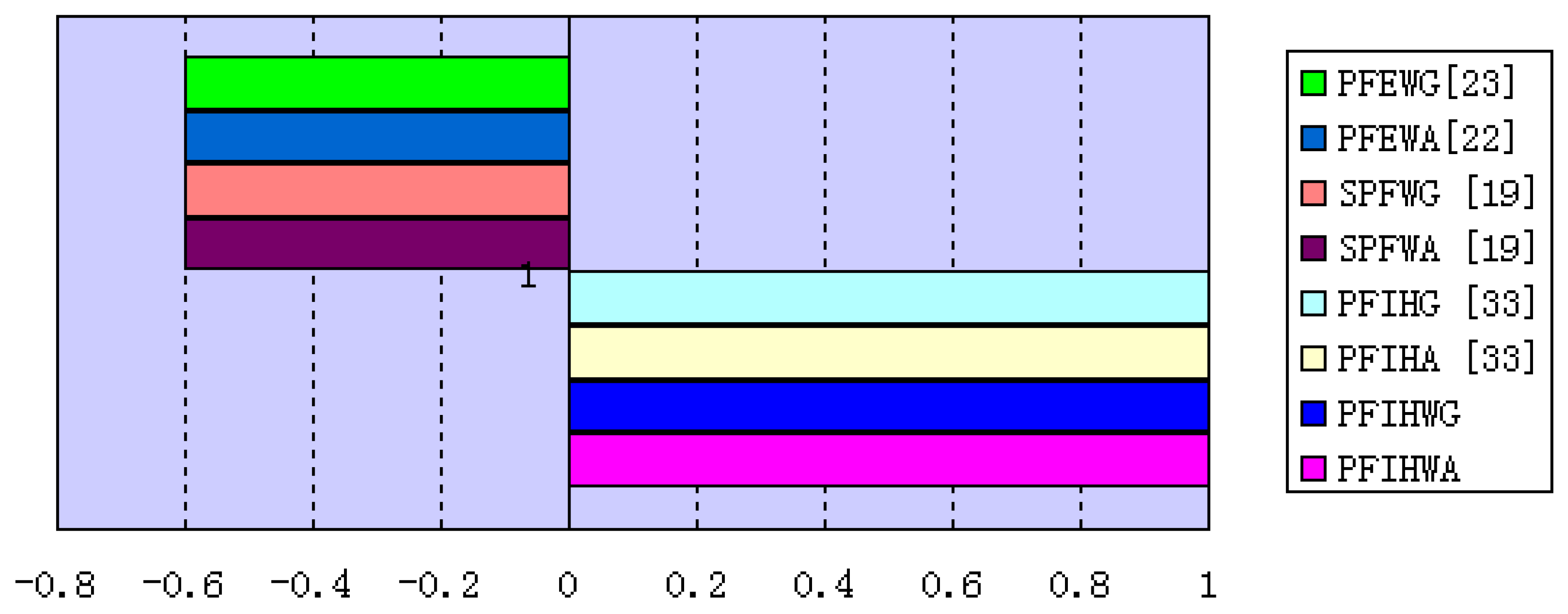
From Figure 1, we observe that the Spearman correlation of SPFWA [19], SPFWG [19], PFEWA [22] and PFEWG [23] are all −0.6, whereas, the Spearman correlation of proposed operator (PFIHWA, PFIHWG), PFIHA [33] and PFIHG [33] are all 1. Comparing with PFIHA [33] and PFIHG [33], the typical characteristics of our techniques are that they possess a small amount of computation and idempotency. It further indicates that our approaches are superior. Therefore, our approach is suitable for settling some practical multiple attribute decision problems with Pythagorean fuzzy information.

5.2. MAGDM Method by Using GPFIHWA and GPFIHWG Operators

Plenty of practical decision-making problems usually demand multiple DMs rather than a single DM. PFSs have the successful capacity to handle the indeterminacy under the MAGDM environment [8,17,25,26,27,28,29,31].

In what follows, we will employ GPFIHWA and GPFIHWG operators to tackle MAGDM problems with PFNs. Assume $A=\{A_1,A_2,\dots ,A_m\}$ and $C=\{C_1,C_2,\dots ,C_n\}$ are respectively the group of alternatives and attributes. The $\epsilon ={({\epsilon }_1,{\epsilon }_2,\dots ,{\epsilon }_n)}^T$ is the weight vector, that meets ${\epsilon }_j\ge 0$,${\displaystyle {\sum }_{j=1}^n{\epsilon }_j=1}$. Suppose $\omega ={({\omega }_1,{\omega }_2,\dots ,{\omega }_n)}^T$ is the associated vector for ${\omega }_j\ge 0$, ${\displaystyle {\sum }_{j=1}^n{\omega }_j=1}$. $D=\{d_1,d_2,\dots ,d_l\}$ is the group of experts, $\tau ={({\tau }_1,{\tau }_2,\dots ,{\tau }_l)}^T$ is the corresponding weight vector that satisfies ${\tau }_k\ge 0$, ${\displaystyle {\sum }_{k=1}^l{\tau }_k=1}$. $R^{(k)}={(r_{ij}^{(k)})}_{m\times n}$ is the assessment matrix, in which $r_{ij}^{(k)}=({\mu }_{r_{ij}^{(k)}},{\nu }_{r_{ij}^{(k)}})$ is a PFN offered by the expert $d_k\in D$ for the alternative $A_i\in A$ relevant to the attribute $C_j\in C$.${\mu }_{r_{ij}^{(k)}}$ and ${\nu }_{r_{ij}^{(k)}}$ means the grade that alternative $A_i$ meets attribute $C_j$ and doesnot meet attribute $C_j$ offered by the expert $d_k$, respectively. Where ${\mu }_{r_{ij}},{\nu }_{r_{ij}}\in [0,1]$, ${({\mu }_{r_{ij}^{(k)}})}^2+{({\nu }_{r_{ij}^{(k)}})}^2\in [0,1]$. Then, the procedure of the MAGDM problem (Algorithm 2) is listed below:

Algorithm 2. The procedure of the MAGDM problem using GPFIHWA and GPFIHWG operators.

Step 1. It is identical with Step 1 in Algorithm 1.

Step 2. Utilize the PFIWA operator and decision matrixes $P^{(k)}={(p_{ij}^{(k)})}_{m\times n}$ to get the group decision matrix $P={(p_{ij})}_{m\times n}$, where $$p_{ij}=\mathrm{PFIWA}(p_{ij}^{(1)},p_{ij}^{(2)},\dots ,p_{ij}^{(l)}).$$

Step 3. Utilize the assessment matrix $P={(p_{ij})}_{m\times n}$ and the GPFIHWA operator $$p_i=\mathrm{GPFIHWA}(p_{i1},p_{i2},\dots ,p_{in})$$ or the GPFIHWG operator $$p_i=\mathrm{GPFIHWG}(p_{i1},p_{i2},\dots ,p_{in})$$ to obtain the comprehensive evaluation values $p_i(i=1,2,3,\dots ,m)$.

Step 4. It is identical with Step 3 in Algorithm 1.

Step 5. It is identical with Step 4 in Algorithm 1.

Example 8.

Suppose a company intends to implement the ERP (Enterprise Resource Planning) system (revised from Reference [28]). Three experts$\{e_1,e_2,e_3\}$from different departments form a project team to make the evaluations, including a CIO(Chief Information Officer) and two senior representatives, whose weight vector is$\tau ={(1/3,1/3,1/3)}^T$. Assume that we have five latent ERP systems$\{A_1,A_2,A_3,A_4,A_5\}$, and four assessment attributes$\{C_1,C_2,C_3,C_4\}$were selected,$C_1$stands for the technology and function;$C_2$stands for the strategic adaptability;$C_3$stands for competence of vendor and$C_4$stands for renown of vendor. Assume$\epsilon ={(0.15,0.2,0.3,0.35)}^T$is the importance degree of attributes. The associated weight vector given by the project team as$\omega ={(0.2,0.1,0.3,0.4)}^T$, which assigns more weight to the attribute obtaining the optimal performance. The five potential ERP systems$A_1,A_2,A_3,A_4,A_5$are appraised by PFNs, and are summarized in

Table 3. The Pythagorean fuzzy decision matrix $R^{(1)}$.

	${\mathit{C}}_1$	${\mathit{C}}_2$	${\mathit{C}}_3$	${\mathit{C}}_4$
$A_1$	(0.4, 0.8)	(0.8, 0.5)	(0.6, 0.7)	(0.3, 0.8)
$A_2$	(0.7, 0.5)	(0.8, 0.4)	(0.8, 0.5)	(0.3, 0.6)
$A_3$	(0.3, 0.4)	(0.3, 0.7)	(0.7, 0.4)	(0.6, 0.4)
$A_4$	(0.6, 0.6)	(0.7, 0.5)	(0.7, 0.2)	(0.4, 0.6)
$A_5$	(0.5, 0.7)	(0.6, 0.4)	(0.9, 0.3)	(0.6, 0.7)

,

Table 4. The Pythagorean fuzzy decision matrix $R^{(2)}$.

	${\mathit{C}}_1$	${\mathit{C}}_2$	${\mathit{C}}_3$	${\mathit{C}}_4$
$A_1$	(0.3, 0.9)	(0.7, 0.6)	(0.5, 0.8)	(0.3, 0.6)
$A_2$	(0.7, 0.4)	(0.9, 0.2)	(0.8, 0.1)	(0.3, 0.5)
$A_3$	(0.3, 0.6)	(0.7, 0.7)	(0.7, 0.6)	(0.4, 0.4)
$A_4$	(0.4, 0.8)	(0.7, 0.5)	(0.6, 0.2)	(0.4, 0.7)
$A_5$	(0.2, 0.7)	(0.8, 0.2)	(0.8, 0.4)	(0.6, 0.6)

and

Table 5. The Pythagorean fuzzy decision matrix $R^{(3)}$.

	${\mathit{C}}_1$	${\mathit{C}}_2$	${\mathit{C}}_3$	${\mathit{C}}_4$
$A_1$	(0.5, 0.8)	(0.7, 0.6)	(0.5, 0.8)	(0.5, 0.5)
$A_2$	(0.6, 0.5)	(0.9, 0.2)	(0.8, 0.1)	(0.3, 0.5)
$A_3$	(0.4, 0.7)	(0.7, 0.5)	(0.6, 0.1)	(0.2, 0.9)
$A_4$	(0.2, 0.9)	(0.5, 0.6)	(0.6, 0.2)	(0.1, 0.6)
$A_5$	(0.1, 0.6)	(0.8, 0.2)	(0.9, 0.2)	(0.6, 0.5)

.

5.2.1. Process of MAGDM based on the GPFIHWA Operator

Step 1. Since every attribute is a benefit type, no transformation is needed. The decision matrix $P^{(k)}={(p_{ij}^{(k)})}_{5\times 4}={(r_{ij}^{(k)})}_{5\times 4}$, is described in Table 3, Table 4 and Table 5.

Step 2. Utilize the PFIWA operator, we get the group decision matrix $P={(p_{ij})}_{5\times 4}$, see

Table 6. The group integrated decision matrix $P$.

	${\mathit{C}}_1$	${\mathit{C}}_2$	${\mathit{C}}_3$	${\mathit{C}}_4$
$A_1$	(0.4114, 0.8371)	(0.7389, 0.5646)	(0.5372, 0.7677)	(0.3832, 0.6579)
$A_2$	(0.6707, 0.4706)	(0.8746, 0.2646)	(0.8000, 0.3493)	(0.3000, 0.5375)
$A_3$	(0.3376, 0.6012)	(0.6176, 0.6992)	(0.6707, 0.4786)	(0.4448, 0.6605)
$A_4$	(0.4448, 0.7739)	(0.6481, 0.5314)	(0.6377, 0.2006)	(0.3357, 0.6436)
$A_5$	(0.3267, 0.6840)	(0.7509, 0.2642)	(0.8746, 0.3015)	(0.6000, 0.6213)

.

Step 3. Utilize the decision matrix $P={(p_{ij})}_{5\times 4}$ and the GPFIHWA operator (suppose $\lambda =2$), from Definition 4, we obtain $s(p_{11})=-0.5314$,$s(p_{12})=0.2271$,$s(p_{13})=-0.3008$, $s(p_{14})=$$-0.2861$. Since, $s(p_{12})>s(p_{14})>s(p_{13})>s(p_{11})$, so $p_{12}\succ p_{14}\succ p_{13}\succ p_{11}$, then $(1)=4,$ $(2)=$$1,$ $(3)=3,(4)=2$. Further, $\frac{{\omega }_{(1)}{\epsilon }_1}{{\displaystyle {\sum }_{j=1}^4{\omega }_{(j)}{\epsilon }_j}}=\frac{0.4\times 0.1}{0.4\times 0.1+0.2\times 0.2+0.3\times 0.35+0.1\times 0.35}=$$0.1818$,$\frac{{\omega }_{(2)}{\epsilon }_2}{{\displaystyle {\sum }_{j=1}^4{\omega }_{(j)}{\epsilon }_j}}=0.1818$, $\frac{{\omega }_{(3)}{\epsilon }_3}{{\displaystyle {\sum }_{j=1}^4{\omega }_{(j)}{\epsilon }_j}}=0.4773$, $\frac{{\omega }_{(4)}{\epsilon }_4}{{\displaystyle {\sum }_{j=1}^4{\omega }_{(j)}{\epsilon }_j}}=0.1591$. According to Equation (15), we obtain $p_1=GPFIHWA(p_{11},p_{12},p_{13},p_{14})=(0.5671,0.7247)$, similarly, $p_2=(0.6256,0.4529)$,$p_3=(0.5426,0.6026)$,$p_4=(0.5470,0.5368)$, $p_5=(0.7311,0.4730)$.

Step 4. Compute the scores of PFNs $p_i(i=1,2,3,4,5)$.

$$s(p_1)=-0.2036, ;s(p_2)=0.1863,s(p_3)=-0.0687,s(p_4)=0.0111,s(p_5)=0.3108.$$

Step 5. Since $s(p_5)>s(p_2)>s(p_4)>s(p_3)>s(p_1)$, then we obtain

$$A_5\succ A_2\succ A_4\succ A_3\succ A_1.$$

Hence, the optimal ERP system is $A_5$.

5.2.2. Process of MAGDM based on the GPFIHWG Operator

Step 1–2. It is the same as Step 1–2 in Section 5.2.1.

Step 3. Utilize the decision matrix $P={(p_{ij})}_{5\times 4}$ and the GPFIHWG operator (suppose $\lambda =2$), by Definition 4, we obtain $s(p_{11})=-0.5314$,$s(p_{12})=0.2271$,$s(p_{13})=-0.3008$, $s(p_{14})=$$-0.2861$. Since, $s(p_{12})>s(p_{14})>s(p_{13})>s(p_{11})$, so $p_{12}\succ p_{14}\succ p_{13}\succ p_{11}$, then $(1)=4,$$(2)=$$1,$$(3)=3,(4)=2$. Further, $\frac{{\omega }_{(1)}{\epsilon }_1}{{\displaystyle {\sum }_{j=1}^4{\omega }_{(j)}{\epsilon }_j}}=\frac{0.4\times 0.1}{0.4\times 0.1+0.2\times 0.2+0.3\times 0.35+0.1\times 0.35}=$$0.1818$,$\frac{{\omega }_{(2)}{\epsilon }_2}{{\displaystyle {\sum }_{j=1}^4{\omega }_{(j)}{\epsilon }_j}}=0.1818$, $\frac{{\omega }_{(3)}{\epsilon }_3}{{\displaystyle {\sum }_{j=1}^4{\omega }_{(j)}{\epsilon }_j}}=0.4773$, $\frac{{\omega }_{(4)}{\epsilon }_4}{{\displaystyle {\sum }_{j=1}^4{\omega }_{(j)}{\epsilon }_j}}=0.1591$. Based on Equation (18), we get $p_1=\mathrm{GPFIHWG}(p_{11},p_{12},p_{13},p_{14})=(0.5265,0.7548)$, similarly,$p_2=(0.5568,0.5352)$,$p_3=(0.5167,0.6249)$,$p_4=(0.4733,0.6028)$,$p_5=(0.6284,0.6029)$.

Step 4. Compute the scores of PFNs $p_i(i=1,2,3,4,5)$.

$$s(p_1)=-0.2925,s(p_2)=0.0236,s(p_3)=-0.1236,s(p_4)=-0.1394,s(p_5)=0.0314.$$

Step 5.$s(p_5)>s(p_2)>s(p_3)>s(p_4)>s(p_1)$, therefore we get

$$A_5\succ A_2\succ A_3\succ A_4\succ A_1.$$

Hence, the optimal ERP system is $A_5$.

5.2.3. Comparison and Discussion

In Step 3 of Section 5.2.2, if we employ the PFIHA and PFIHG operators [33], then the decision result is $A_5\succ A_2\succ A_3\succ A_4\succ A_1$. If we use the SPFWA [19], SPFWG [19], PFEWA [22] and PFEWG [23] operators, we obtain the following result: $A_2\succ A_5\succ A_4\succ A_3\succ A_1$. We can obtain that the decision outcomes by the PFIHA operator [33] and PFIHG operator [33] are the same as our GPFIHWG operator, and are slightly different with our GPFIHWA operator, but the most desirable alternative by the PFIHA and PFIHG operators [33] coincide with the proposed operator results, i.e., alternative $A_5$. The most desirable alternative determined by SPFWA [19], SPFWG [19], PFEWA [22] and PFEWG [23] operators is $A_2$ for all, the reason is that these AOs do not consider the interaction among membership and non-membership grades. Therefore, it is available and feasible in the proposed approaches. 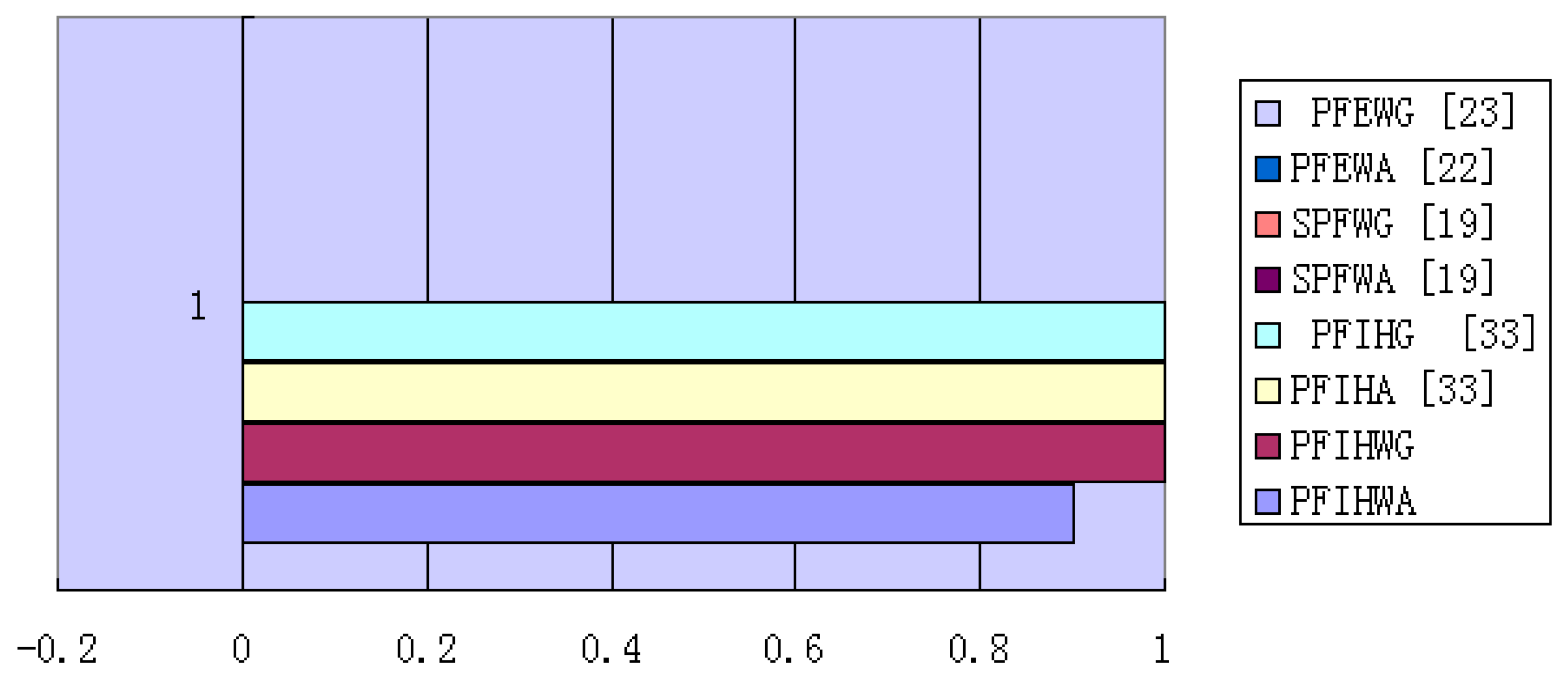Moreover, our approaches are simple from the computational point of view compared with the PFIHA and PFIHG operators [33]. Further contrast effect can be reflected in Figure 2.

As provided in Figure 2, the Spearman correlations of SPFWA [19], SPFWG [19], PFEWA [22] and PFEWG [23] are all 0, which shows that our methods are superior. The main features of the proposed GPFIHWA and GPFIHWG operators are that: (1) it considers the interaction among membership and non-membership grades for PFNs, and are more suitable to address actual MADM issues in some special situations; (2) it has the property of idempotency and simple computation process; (3) it possess an adjust parameter value and can reflect the preference of DMs during the decision process.

5.2.4. Sensitivity Analysis

Parameter $\lambda$ plays a significant influence in the decision-making process; it can reflect the mentality of the DMs. For this, we chose different values of $\lambda$ from 0 to 30 in Algorithm 2 to solve Example 8, so as to investigate the flexibility and sensitivity of different $\lambda$. The scores as well as decision results are listed in

Table 7. The scores and ranking results by the generalized Pythagorean fuzzy interactive hybrid weighted average (GPFIHWA) operator with different parameter $\lambda$.

$\mathit{\lambda }$	$\mathit{s}({\mathit{p}}_1)$	$\mathit{s}({\mathit{p}}_2)$	$\mathit{s}({\mathit{p}}_3)$	$\mathit{s}({\mathit{p}}_4)$	$\mathit{s}({\mathit{p}}_5)$	Ranking
$0$	−0.2582	0.1449	−0.0889	−0.1180	0.1538	$A_5\succ A_2\succ A_3\succ A_4\succ A_1$
1	−0.2352	0.2018	−0.0838	−0.0797	0.2686	$A_5\succ A_2\succ A_4\succ A_3\succ A_1$
2	−0.2036	0.1863	−0.0687	0.0111	0.3108	$A_5\succ A_2\succ A_4\succ A_3\succ A_1$
4	−0.1277	0.1890	−0.0338	0.1877	0.3623	$A_5\succ A_2\succ A_4\succ A_3\succ A_1$
7	−0.0422	0.2334	0.0108	0.3015	0.4137	$A_5\succ A_4\succ A_2\succ A_3\succ A_1$
11	0.0265	0.2732	0.0544	0.3580	0.4574	$A_5\succ A_4\succ A_2\succ A_3\succ A_1$
16	0.0751	0.3061	0.0906	0.3936	0.4903	$A_5\succ A_4\succ A_2\succ A_3\succ A_1$
22	0.1085	0.3337	0.1175	0.4183	0.5138	$A_5\succ A_4\succ A_2\succ A_3\succ A_1$
30	0.1341	0.3586	0.1384	0.4381	0.5326	$A_5\succ A_4\succ A_2\succ A_3\succ A_1$

and

Table 8. The scores and ranking results by the generalized Pythagorean fuzzy interactive hybrid weighted geometric (GPFIHWG) operator with different parameter $\lambda$.

$\mathit{\lambda }$	$\mathit{s}({\mathit{p}}_1)$	$\mathit{s}({\mathit{p}}_2)$	$\mathit{s}({\mathit{p}}_3)$	$\mathit{s}({\mathit{p}}_4)$	$\mathit{s}({\mathit{p}}_5)$	Ranking
$0$	−0.2352	0.2018	−0.0838	−0.0797	0.2686	$A_5\succ A_2\succ A_4\succ A_3\succ A_1$
1	−0.2582	0.1449	−0.0889	−0.1180	0.1538	$A_5\succ A_2\succ A_3\succ A_4\succ A_1$
2	−0.2925	0.0236	−0.1236	−0.1394	0.0314	$A_5\succ A_2\succ A_3\succ A_4\succ A_1$
4	−0.3422	−0.1775	−0.1858	−0.1915	−0.1228	$A_5\succ A_2\succ A_3\succ A_4\succ A_1$
7	−0.3785	−0.2928	−0.2316	−0.2351	−0.2272	$A_5\succ A_3\succ A_4\succ A_2\succ A_1$
11	−0.4069	−0.3377	−0.2642	−0.2648	−0.3058	$A_3\succ A_4\succ A_5\succ A_2\succ A_1$
16	−0.4328	−0.3594	−0.2907	−0.2865	−0.3662	$A_4\succ A_3\succ A_2\succ A_5\succ A_1$
22	−0.4550	−0.3731	−0.3134	−0.3027	−0.4095	$A_4\succ A_3\succ A_2\succ A_5\succ A_1$
30	−0.4748	−0.3836	−0.3355	−0.3164	−0.4433	$A_4\succ A_3\succ A_2\succ A_5\succ A_1$

.

Table 7 indicates that the scores in the GPFIHWA operator become bigger with parameter $\lambda$ increasing. Therefore, the DMs with optimistic attitude should take larger values of $\lambda$. Moreover, the ranking results are different by using different values of $\lambda$, but the best alternative is always $A_5$. Furthermore, we can find that

(1)

(1) when $\lambda \in (0,0.8765]$, the ranking is $A_5\succ A_2\succ A_3\succ A_4\succ A_1$.

(2)

when $\lambda \in (0.8765,4.0562]$, the ranking is $A_5\succ A_2\succ A_4\succ A_3\succ A_1$.

(3)

when $\lambda \in (4.0562,30]$, the ranking is $A_5\succ A_4\succ A_2\succ A_3\succ A_1$.

Table 8 indicates that the scores in the GPFIHWG operator become smaller with parameter $\lambda$ increasing. Therefore, the DMs with optimistic attitude should take smaller values of $\lambda$. Moreover, the ranking results are also different by employing different values of $\lambda$, and the best alternative is from $A_5$ to $A_3$, then from $A_3$ to $A_4$ with parameter $\lambda$ increasing. Furthermore, we can find that

(1)

when $\lambda \in (0,0.1235]$, the ranking is $A_5\succ A_2\succ A_4\succ A_3\succ A_1$,

(2)

when $\lambda \in (0.1235,4.3582]$, the ranking is $A_5\succ A_2\succ A_3\succ A_4\succ A_1$,

(3)

when $\lambda \in (4.3582,4.5858]$, the ranking is $A_5\succ A_3\succ A_2\succ A_4\succ A_1$,

(4)

when $\lambda \in (4.5858,7.3828]$, the ranking is $A_5\succ A_3\succ A_4\succ A_2\succ A_1$,

(5)

when $\lambda \in (7.3828,7.6462]$, the ranking is $A_3\succ A_5\succ A_4\succ A_2\succ A_1$,

(6)

when $\lambda \in (7.6462,11.6251]$, the ranking is $A_3\succ A_4\succ A_5\succ A_2\succ A_1$,

(7)

when $\lambda \in (11.6251,15.1215]$, the ranking is $A_4\succ A_3\succ A_5\succ A_2\succ A_1$,

(8)

when $\lambda \in (15.1215,30]$, the ranking is $A_4\succ A_3\succ A_2\succ A_5\succ A_1$.

Therefore, the approach by using the GPFIHWA operator is relatively stable. In the actual decision environment, the DMs may select a different parameter $\lambda$ in line with their preferences.

To better distinguish the presented approach with the existing approaches [19,22,23,33,37,38,39], we summarize the differences of them in

Table 9. Characteristic comparisons of different methods.

Methods	Considers the Interactions between Membership and Non-Membership	Possesses the Property of Idempotency
PFIHA [33]	Yes	No
PFIHG [33]	Yes	No
SPFWA [19]	No	Yes
SPFWG [19]	No	Yes
PFEWA [22]	No	Yes
PFEWG [23]	No	Yes
Liao and Xu [40]	No	Yes
Our proposed operators	Yes	Yes

. Based on Table 9, we can obtain that the presented approaches possess the property of idempotency, and also embody the interactions among membership and non-membership during the information aggregation process. Therefore, the novel approaches can obtain more reasonable ranking results.

6. Conclusions

In this study, the authors have presented a group of novel Pythagorean fuzzy interactive hybrid weighted AOs, such as the PFIHWA, PFIHWG, GPFIHWA and GPFIHWG operators. It can be seen that these novel developed operators have the feature of idempotency, which indicated that the proposed AOs could overcome the shortcomings of the PFIHA and the PFIHG operators. It was also shown that some other existing AOs [33,35] were the particular cases of our presented AOs. In addition, our approaches were simple in view of computational cost and also captured the interaction over membership and non-membership grades. Afterward, two algorithms to MADM and MAGDM by the proposed operators were provided. Lastly, we verified the validity and flexibility with two practical examples.

In future research work, we can expand the explored operators to neutrosophic set [42,43,44], q-rung orthopair fuzzy set [45,46,47] and other uncertain environments [48,49,50,51,52,53,54,55,56].