A Compact Representation of Preferences in Multiple Criteria Optimization Problems

Abstract

A critical step in multiple criteria optimization is setting the preferences for all the criteria under consideration. Several methodologies have been proposed to compute the relative priority of criteria when preference relations can be expressed either by ordinal or by cardinal information. The analytic hierarchy process introduces relative priority levels and cardinal preferences. Lexicographical orders combine both ordinal and cardinal preferences and present the additional difficulty of establishing strict priority levels. To enhance the process of setting preferences, we propose a compact representation that subsumes the most common preference schemes in a single algebraic object. We use this representation to discuss the main properties of preferences within the context of multiple criteria optimization.

1. Introduction

Setting preferences in multiple criteria optimization problems may have an important influence on the final selection of the best solutions. However, it is usually assumed in the literature that preferences are somehow given by the decision-maker to the analyst. Then, the focus is placed on methodology disregarding some important features that may result critical in eliciting solutions. These features include (1) cardinality, when preferences are given in terms of weights attached to criteria; (2) ordinality, when preferences are expressed as a criteria order; and (3) clustering, when preferences are grouped in hierarchies or noncontinuous levels with non-finite preferences among criteria.

Eliciting weights that accurately represent the preferences of decision-makers is a key issue in multiobjective optimization [1]. To some extent, expressing weights implies the assumption of some knowledge about the impact that these weights have on the performance of alternative decisions. Indeed, decision-makers usually express their preferences for alternative solutions in terms of the set of criteria under consideration [2]. Furthermore, weight setting in the context of multiobjective optimization is also an interactive process in which decision-makers play a relevant role [3].

Several methodologies have been proposed to compute the relative priority of criteria when preference relations can be expressed either by ordinal or by cardinal information. On the one hand, the analytic hierarchy process (AHP) proposed in [4] introduces relative priority levels and cardinal preferences. A broad range of recent AHP applications can be found in many different disciplines dealing with environmental problems [5,6,7], health [8], finance [9], and product development [10]. On the other hand, lexicographical orders [11,12] combine both ordinal and cardinal preferences and present the additional difficulty of establishing strict priority levels where preferences among criteria are noncontinuous. Some recent examples of lexicographic optimization applications include the optimization of water resources planning [13], electricity market clearing [14], and combined heat and power scheduling [15].

Despite sharing a common goal, namely, establishing priorities between decision-making objectives, there is no unifying approach to represent and setting preferences derived from the analysis of AHP and lexicographic orders. Furthermore, decision-makers can express their opinions by means of ordinal or cardinal information, but they need to represent it in a suitable way to make computations in the optimization process [16]. In this paper, we provide a compact representation of preferences that generalizes cardinal, ordinal, and clustering approaches to manage the relative importance of goals in a single algebraic object. This compact representation is based on the concept of powerset, which includes all possible subsets that can be formed from a given set of goals. Our representation aims to improve the interactive process of setting preferences. It facilitates the understanding and it allows further analysis on the main properties of different preference setting options. In addition, we explore the main properties of powerset preference rules within the context of multiple criteria optimization problems. Summarizing, three important contributions must be highlighted:

• We introduce the concept of powerset preference rule that generalizes previous approaches such as AHP and lexicographical orders.
• We provide a unique and compact representation of preferences for objectives based on both ordinal and cardinal information.
• We propose two theoretical results on the properties of powerset preference rules, namely, alignment, and preference order.

As the influence of preference setting in the solution of an optimization problem may be remarkable, we argue that this analysis may result fruitful for decision-makers in several ways. First, we establish a link between AHP and lexicographical orders, as both methodologies are more related than it may seem at first glance. Indeed, both methods aim to express preferences for different objectives. Second, we solve the problem of combining both ordinal and cardinal information by relying on the concept of powerset preference rule. We also combine both clusters of objectives and complex hierarchical structures in a single algebraic object. Third, from the analysis of the main properties of powerset preference rules, decision-makers can better understand the implications and importance of weight setting through the common interactive process in multiobjective optimization. Detection of inconsistencies and a more effective way to develop this interactive process are the main benefits that decision-makers can derive from the proposal described in this paper. In addition, researchers have now the opportunity to propose new theoretical results, as this compact representation and the definition of powerset preference rules pave the way to formal reasoning.

In addition to this introduction, this paper includes Section 2, where useful background on setting preferences multicriteria optimization problems is given. Section 3 is the central part of this paper where the concept of powerset preference rule is introduced. Section 4 explores the main properties of powerset preference rules, and Section 5 concludes.

2. Setting Preferences in Multicriteria Optimization Problems

The concept of attribute refers to interesting values for a decision-maker that related to an objective reality that can be measured [12]. Let us assume that these measures can be expressed by means of a general mathematical function $g_i\left(\mathit{x}\right)$ that ultimately depends on vector of solutions $\mathit{x}$ within feasible set $\mathcal{X}$. From the set of all possible attributes, decision-makers select those that result of interest for them. In addition, they establish the desired direction of improvement (maximization or minimization) and some aspiration levels (if any). As a result, attributes are transformed in given a set of criteria $\mathcal{G}=\{g_1\left(\mathit{x}\right),g_2\left(\mathit{x}\right),\dots ,g_q\left(\mathit{x}\right)\}$. From this set, a general multicriteria optimization problem can be formulated under a maximization point of view:

$$\max \left[g_1\left(\mathit{x}\right),g_2\left(\mathit{x}\right),\dots ,g_q\left(\mathit{x}\right)\right]$$

(1)

subject to

$$\mathit{x}\in \mathcal{X}.$$

(2)

Each function $g_i\left(\mathit{x}\right)$ is a measure of the achievement of the i-th criterion. However, the presence of multiple criteria requires setting specific preferences, priorities, or weights to express the relative importance of the achievement of each criterion. For instance, if $g_1\left(\mathit{x}\right)$ measures return and $g_2\left(\mathit{x}\right)$ measures safety of an investment $\mathit{x}$, but return is assessed by a decision-maker to be twice more important than safety, we can reasonably use the following weighted objective function,

$$w_1·g_1\left(\mathit{x}\right)+w_2·g_2\left(\mathit{x}\right)=0.67·g_1\left(\mathit{x}\right)+0.33·g_2\left(\mathit{x}\right).$$

(3)

Note that Equation (3) is a scalarizing function [17] used as a surrogate to measure global achievement according to the particular preferences for a decision-maker. These preferences are expressed by means of cardinal information, i.e., by means of weights $w_1$ and $w_2$. However, preferences for criteria can also be expressed using ordinal information by establishing strict priority levels of criteria, as in the case of lexicographical optimization [11,12]. The fulfillment of some criteria are immeasurably preferred to the fulfillment of another set of criteria. Criteria are then classified in groups, priority levels, or clusters and the preference among clusters may be either finite (AHP) or infinite (lexicographical orders). In addition, if several criteria are at the same priority level, cardinal information is used to expressed preferences among criteria within the level [18].

To facilitate the analysis, criteria (and clusters of criteria) can be organized in complex structures such as hierarchies or networks. The analytic hierarchy process (AHP) proposed by [4], and its generalization—the analytic network process (ANP) [19]—is the most common approach to set preferences in a multicriteria context. The relative importance of criteria and the final priorities are computed considering the relationship between clusters of criteria and the specific priority established among criteria within a cluster.

Summarizing, we find in the literature three main approaches to set preferences in a multicriteria optimization context: (1) A basic approach when the number of criteria is small as described in Equation (3); (2) AHP: when complex structures are used to establish cardinal priorities; and (3) lexicographical orders: when ordinal information is required to set strict priority levels between clusters and, at the same time, cardinal information is used to establish numerical preferences among criteria within a cluster. The main features of these approaches are summarized in

Table 1. Features of main approaches to set preferences.

Approach	Cardinal	Ordinal	Clustering
Basic	√
AHP/ANP	√		√
Lexicographical	√	√	√

. Next, we consider these last two approaches in more detail.

2.1. Analytic Hierarchy Process

The AHP [4] has become one of the most widely used tools in the resolution of complex decision-making problems. All the pairwise comparisons generated by the relative weights of the criteria represent judgments made by decision-makers. The AHP provides a systematic process to incorporate factors such as logic, experience or knowledge, emotion, and a sense of optimization into a decision-making methodology [20]. A detailed description of the AHP method can be found in [21]. AHP has been applied in a broad range of application areas [22,23]. There has been a steady-state increase in its usage since its introduction, due to its ease of application. A large body of research concerning with AHP applications in different disciplines can be found in literature including, but not limited to, wastewater services [7], new product development [10], Internet finance [9], sustainable and renewable energy [24,25], water resources management [5,6], agriculture [26], health [8], nuclear power [27], climate change [28], and presidential elections [29].

A useful tool to set and work with preferences in AHP is a comparison matrix. For each cluster of criteria of size n, decision-makers establish specific preferences by setting element $a_{ij}$ of matrix $A\in {\mathbb{R}}^{n\times n}$ to a numeric value. As an illustrative example, let us consider the concept of sustainability. The intersection of economic, social, and environmental criteria is usually known as sustainability [30]. While designing public policies, a government may be interested in sustainable policies, namely, those that consider not only economic but also social and environmental aspects. As a result, we are dealing with a multiple criteria decision-making problem, but we need to set preferences in the achievement of the economic, social, and environmental criteria. AHP relies on a numerical scale and a pairwise comparison matrix to set these priorities. The numerical scale ranges from 1 (both criteria are equally important) to 9 (one criterion is extremely more important than another one). An example of the pairwise comparison between economic, social and environmental criteria is summarized in

Table 2. Establishing priorities between economic, social, and environmental criteria.

	Economic	Social	Environmental	Sum	Priorities
Economic	1	1/7	1/3	1.5	0.09
Social	7	1	3	11.0	0.65
Environmental	3	1/3	1	4.3	0.26
Total				16.8	1.00

.

According to the numerical scale proposed by Saaty, the social criterion is very strongly more important than the economic one and the environmental criterion is moderately more important than the economic one. Finally, the social criterion is moderately more important than the environmental one. To obtain the final priorities following the approximate method proposed by Saaty, we sum the values of each row and divide by the sum of all judgments. Alternatively, we can normalize the judgments in any column by dividing each entry by the sum of that column and by averaging normalized values for each row. However, rather than the method to establish priorities, in this paper, we focus on the representation of preferences and its main properties. The algebraic object equivalent to Table 2 is the following matrix,

$$A=\left[\begin{array}{ccc}\hfill 1& \hfill 1/7& \hfill 1/3\\ \hfill 7& \hfill 1& \hfill 3\\ \hfill 3& \hfill 1/3& \hfill 1\end{array}\right].$$

(4)

Note that the AHP implies reciprocal judgments, meaning that $a_{ij}=1/a_{ji}$. In addition, consistency is a desired property. Here, perfect consistency means that $a_{ik}=a_{ij}·a_{jk}$. That is, if the social criterion is moderately more important than the environmental criterion and, at the same time, the environmental criterion is moderately more important than the economic criterion, the social criterion should be extremely more important than the economic criterion for consistency. Note that consistency does not perfectly holds in matrix A, as $a_{13}=0.33$ is not exactly $a_{12}·a_{23}=0.43$. Although some level of inconsistency can be accepted, decision-makers must check this property when setting preferences. An additional requirement of the AHP is the homogeneity of elements to be compared, as ranges are restricted to the scale of 1 to 9. We cannot compare a grain of sand to a mountain.

However, the main feature of the AHP is that preferences are established hierarchically, meaning that more general criteria subsume specific criteria. A hierarchy can be represented graphically as a parent node and several child nodes linked to it as shown in Figure 1. This graph defines the relative importance that subcriteria (growth, risk, and profits) have on a parent node (economic). Priorities among the subcriteria are then established by clusters (growth, risk, and profits on the one hand, and social, economic, and environmental performance on the other hand). Then, the relative importance of lower-level criteria (growth, risk, and profits) on the overall goal (sustainability) is weighted by the priority of the economic criterion with respect to same-level criteria (social and Environmental). As a result, we need a comparison matrix for each of the clusters in the hierarchy. Finally, each criterion in the hierarchy has an influence in the overall criterion (Sustainability).

2.2. Lexicographic Orders

The lexicographic approach to multiobjective optimization was first introduced by [31] and later developed mainly by [18,32]. Lexicographic orders [1,11,12,33] are useful when a decision-maker has a predefined ordering of criteria. Because of that, lexicographic optimization is also known as preemptive optimization. In lexicographic orders, optimization is organized in strict priority levels, meaning that higher priority levels are infinitely more important than lower priority levels for optimization purposes. There is no trade-off between the achievement goals in different priority levels. The achievement of goals in a higher priority level are immeasurably preferred to the achievement of goals in a lower priority level. However, the achievement levels of other priority level goals can also be determined, therefore allowing an interesting sensitivity analysis [34]. As a result, optimization takes place in a sequential manner. Optimal solutions for higher priority levels are considered as invariant input data for lower level optimization.

Some examples of the use of lexicographic orders in multiple criteria optimization are the following. The authors of [32] proposed a lexicographic goal program to select projects or investment opportunities from a given finite set to maximize profits as a first priority and market share as a second priority. The authors of [34] tackled natural resource planning problems with economic, environmental, and social criteria in the development of forest energy plantations in Eastern Ontario by means of lexicographic goal programming. The authors of [13] described the optimization of water resources planning for Lago Maggiore in Italy to maximize flood protection, minimize supply shortage for irrigation, and maximize electricity generation where the order of objectives is strict and prescribed by law. More recently, the authors of [14] proposed a multi-objective lexicographic optimization framework for electricity market clearing, and the authors of [15] relied on lexicographic orders for combined heat and power scheduling.

As criteria placed in a higher priority level are strictly preferred to those placed in a lower priority level, cardinal, or numerical information is not appropriate to set preferences between priority levels. Instead, we require ordinal information to establish preferences, namely, a binary relation between priority levels. In the hierarchy represented in Figure 1, if we assume that the Economic criterion is strictly preferred to the Social criterion and, at the same time, the Social criterion is strictly preferred, we are dealing with the following lexicographic maximization problem,

$$\mathrm{Lex}\max \left[g_1\left(\mathit{x}\right),g_2\left(\mathit{x}\right),g_3\left(\mathit{x}\right)\right]$$

(5)

subject to

$$\mathit{x}\in \mathcal{X}$$

(6)

where $g_1\left(\mathit{x}\right)$, $g_2\left(\mathit{x}\right)$, and $g_3\left(\mathit{x}\right)$ represent, respectively, the achievement of the Economic, Social, and Environmental criteria. Here, the order of goals in expression (5) is very important, as it is only when goal $g_1\left(\mathit{x}\right)$ is optimized that goal $g_2\left(\mathit{x}\right)$ is considered, and, in turn, it is only when $g_2\left(\mathit{x}\right)$ is optimized that $g_3\left(\mathit{x}\right)$ is considered. Goals are then ordered as the words in a dictionary. However, we can find numerical preferences among the criteria within the same priority level. In the example shown in Figure 1, a conservative manager may consider risk twice more important than growth and profits. The lexicographic maximization of Equation (5) should then be expanded to consider the relative importance of the subcriteria that form the Economic criterion.

$$\mathrm{Lex}\max \left[0.5g_4\left(\mathit{x}\right)+0.25g_5\left(\mathit{x}\right)+0.25g_6\left(\mathit{x}\right),g_2\left(\mathit{x}\right),g_3\left(\mathit{x}\right)\right]$$

(7)

where $g_4\left(\mathit{x}\right)$, $g_5\left(\mathit{x}\right)$, and $g_6\left(\mathit{x}\right)$ represent, respectively, the achievement of the Risk, Growth, and Profits criteria. As a result, lexicographic multicriteria optimization requires representing preferences by means of both cardinal (numerical) and ordinal (binary) information. This information can be summarized in numerical matrices, as in the case of the AHP, and also in Boolean matrices to set priority levels. Next, we propose a compact representation of preferences that subsumes AHP and Lexicographic orders in a single algebraic object.

3. A Compact Preference Representation

In Section 1, we considered two different ways of representing preferences: (1) the measurable way, when preferences are expressed by cardinal information (AHP), and (2) the immeasurable way, when preferences are expressed by a ordinal information (lexicographical orders). In addition, both the AHP and lexicographical orders imply the definition of some degree of hierarchical dependence among criteria. These two approaches require the use of several matrices to represent the global set of preferences for multiple criteria. Next, we rely on the concept of powerset preference rule to provide a compact representation of preferences by means of a single algebraic object, namely, a matrix.

3.1. A Compact Representation of AHP Preferences

In multiple criteria optimization problems, setting the preferences for the criteria that are important to decision-makers is a key issue. Given a set of criteria $\mathcal{G}=(g_1\left(\mathit{x}\right),g_2\left(\mathit{x}\right),\dots ,g_q\left(\mathit{x}\right))$, the main goal is to establish a set of priorities or weights for each criterion to derive the solutions. These priorities state when and how much a criterion is preferred to another. To this end, AHP [4] is based on binary relations among criteria.

Definition 1.

Binary relation. Given a set $\mathcal{G}$, a binary relation is a subset of $\mathcal{G}\times \mathcal{G}$.

Let us consider a binary relation ⪰, meaning at-least-as-good-as, defined on set $\mathcal{G}$ with cardinality $q=\left|\mathcal{G}\right|$. In the case of AHP [4], a pairwise comparison is a map from a binary relation to a numerical value: $\phi :\mathcal{G}\times \mathcal{G}\to \mathbb{R}$. The partial result is a positive real variable $a_{ij}$, which reveals some degree of preference within the interval $\left[1/9,9\right]$ among criteria i and j, namely, $g_i⪰g_j$. Additionally, the global result is a $q\times q$ matrix of preferences A as in matrix (4). In this example, goal $g_2$ is assessed by the decision-maker to be strongly more important than $g_1$, and $g_3$ moderately more important than $g_1$. According to the numerical equivalence described in [4], this assessment implies setting element $a_{21}$ of matrix A to 7 and $w_{31}$ to 3. Similarly, $g_2$ is assessed to be moderately more important than $g_3$. This assessment implies setting element $w_{23}$ to 3. For reciprocity, element $a_{ij}$ is set to the inverse of element $a_{ji}$, and elements $a_{ii}$ are set to 1, meaning that goals are equally important. For coherence, element $a_{ik}\approx a_{ij}·a_{jk}$, meaning that if goal i is more important than goal j and j is more important than k, then i should be more important than k. Summarizing, preferences are expressed by means of a binary relation and a preference rule (see, e.g., in [4]).

Definition 2.

Preference rule. Given a set of criteria $\mathcal{G}$, a preference rule is a map $\phi :\mathcal{G}\times \mathcal{G}\to Y$, where Y is a set of numbers.

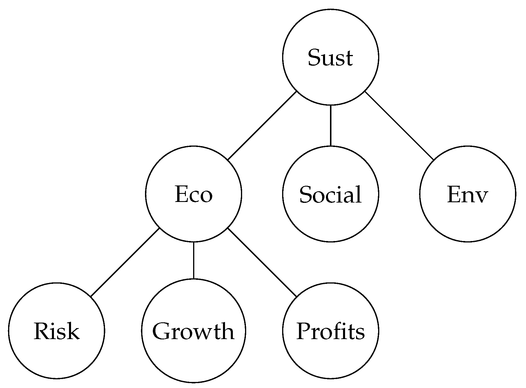
This numerical assessment (preference rule) is usually summarized in a matrix. Due to its hierarchical structure, AHP requires the use of a different matrix to establish preferences for criteria within the same level. In Figure 1, a root node ($g_1$, Sustainability) subsumes the Social, Economic, and Environmental criteria within the same level. Risk, Growth, and Profits belong to a different level. However, we can integrate all matrices in a single block matrix. Let $A_1$ be the $3\times 3$ pairwise comparison matrix for the first level, with Social, Economic, and Environmental criteria identified as $g_2$, $g_3$, and $g_4$, respectively. Let $A_2$ be the $3\times 3$ pairwise comparison matrix for the second level with Risk, Growth, and Profits, denoted by $g_5$, $g_6$, and $g_7$, respectively. By considering an additional $3\times 3$ matrix $A_0$ with all its elements set to zero, we can summarize these preferences by means of a $6\times 6$ block matrix as follows,

$$A=\left[\begin{array}{cc}\hfill A_1& \hfill A_0\\ \hfill A_0& \hfill A_2\end{array}\right].$$

(8)

Note that the size of $A_0$ is chosen to satisfy the requirement that A is a square matrix, and that in the case where the sizes of $A_1$ and $A_2$ are different, we would require two matrices, namely, $A_0$ and $A_0^{\prime }$, with different sizes. This preference representation does not provide information about the hierarchical structure described in Figure 1. As it is typical in graph theory, we can represent this hierarchical structure using an adjacency matrix Z with element $z_{ij}$ set to 1 if there is a relation between criteria i and j, zero otherwise. By convention, we consider that nodes are not connected to themselves by setting $z_{ii}=0$.

$$Z=\left[\begin{array}{ccccccc}\hfill 0& \hfill 1& \hfill 1& \hfill 1& \hfill 0& \hfill 0& \hfill 0\\ \hfill 1& \hfill 0& \hfill 0& \hfill 0& \hfill 1& \hfill 1& \hfill 1\\ \hfill 1& \hfill 0& \hfill 0& \hfill 0& \hfill 0& \hfill 0& \hfill 0\\ \hfill 1& \hfill 0& \hfill 0& \hfill 0& \hfill 0& \hfill 0& \hfill 0\\ \hfill 0& \hfill 1& \hfill 0& \hfill 0& \hfill 0& \hfill 0& \hfill 0\\ \hfill 0& \hfill 1& \hfill 0& \hfill 0& \hfill 0& \hfill 0& \hfill 0\\ \hfill 0& \hfill 1& \hfill 0& \hfill 0& \hfill 0& \hfill 0& \hfill 0\end{array}\right].$$

(9)

Note that matrix Z is symmetric, as elements $z_{12}$, $z_{13}$, and $z_{14}$ set to one require that their reciprocals ($z_{21}$, $z_{31}$, and $z_{41}$, respectively) are also set to one, showing that there is a relation between criteria $g_1$ and subcriteria $g_4$, $g_5$, and $g_6$. By merging matrices A and Z into a larger matrix, we could obtain a global representation of preferences and the relationship among criteria. However, to provide a more compact representation of AHP preferences, we use the concept of powerset [35].

Definition 3.

Powerset. Given a set of criteria $\mathcal{G}$, the powerset of $\mathcal{G}$, denoted by $2^{\mathcal{G}}$, is the set of all subsets of $\mathcal{G}$, including the empty set and $\mathcal{G}$ itself.

As an illustrative example, given $\mathcal{G}=(g_1,g_2)$, the powerset of $\mathcal{G}$ is

$$2^{\mathcal{G}}=(\varnothing ,g_1,g_2,(g_1,g_2)).$$

(10)

Note that if $q=\left|\mathcal{G}\right|$ is the cardinality of $\mathcal{G}$, the cardinality of $2^{\mathcal{G}}$ is $\left|2^{\mathcal{G}}\right|=2^q$. Then, to establish a hierarchical structure in which a subset of goals are clustered for comparison purposes, we next introduce the concept of powerset preference rule as follows.

Definition 4.

Powerset preference rule. Given a set of criteria $\mathcal{G}$, a powerset preference rule is a map $\phi :2^{\mathcal{G}}\times 2^{\mathcal{G}}\to Y$, where Y is a set of numbers.

Let us consider the following powerset preference rule $\phi :2^{\mathcal{G}}\times 2^{\mathcal{G}}\to \mathbb{R}$,

$$\phi (Q_i,Q_j)=\left\{\begin{array}{ccc}{a}_{ij}\in \left[1,9\right]\hfill & \mathrm{if}\hfill & Q_i⪰Q_j,\hfill \\ 1/a\hfill & \mathrm{if}\hfill & Q_i⪯Q_j,\hfill \\ 0\hfill & & otherwise.\hfill \end{array}\right.$$

(11)

where $Q_i$ and $Q_j$ are subsets of $\mathcal{G}$, and $a_{ij}$ is an integer number restricted to the interval $\left[1,9\right]$, as it is customary in AHP to describe a cardinal binary relation ⪯ among pairs of goals. This powerset preference rule allows us to compactly represent AHP preferences including clusters (subsets) of goals that are related in a hierarchical mode. Then, by replacing the economic goal with subset (R,G,P), denoting Risk, Growth, and Profits, we can compactly represent AHP preferences as shown in

Table 3. A compact preference representation of analytic hierarchy process (AHP) where (R, G, P) = (Risk, Growth, Profits).

	(R, G, P)	Soc	Env	Risk	Growth	Profits
(R, G, P)	1	1/7	1/3	0	0	0
Soc	7	1	3	0	0	0
Env	3	1/3	1	0	0	0
Risk	0	0	0	1	1	1
Growth	0	0	0	1	1	1
Profits	0	0	0	1	1	1

. Subset (R,G,P) is at the same hierarchical level than the Social and Environmental goals. In turn, Risk, Growth, and Profits within subset (R,G,P) are equally important according to the information provided by the decision-maker. As a result, the hierarchical structure of AHP and its preferences are both completely and compactly described by a powerset preference rule as in Equation (11).

Note that Table 3, as an example of the output derived form the preference rule in Equation (11), is a different object than the supermatrix described in [19]. A supermatrix summarizes the influences of a set of elements in a cluster of criteria on any other element. These influences are represented by weight vectors derived from pairwise comparisons between criteria. Here, we represent these pairwise comparisons (including individual criteria and sets of criteria) and the particular relationship between criteria in a more compact way by means of a single algebraic object. Nevertheless, the supermatrix can also be derived from the representation of preferences proposed in this work.

To better illustrate our proposal, we next use a real example from recent literature. Consider the credit evaluation for Internet finance companies in [9]. The authors use a survey within an AHP configuration described in

Table 4. Hierarchy of criteria $\mathcal{G}$ described in [9].

Criterion Layer	Index Layer	Second Index Layer
A1 Financial status	B1 Debt Solvency	C1 Debt/assets ratio
		C1 Current ratio
		C3 Quick ratio
		C4 Cash ratio
	B2 Profitability	C5 Profit ratio
		C6 Return on assets
	B3 Operational capacity	C7 Inventory turnover
		C8 Receivable turnover
A2 Credit status	B4 Loan repayment
	B5 Payment capability
	B6 Taxes capability
A3 Enterprise development	B7 Operators quality
	B8 Staff quality
	B9 Prospects
A4 Internet financial status	B10 Customer evaluation
	B11 Logistics
	B12 Turnover index

to propose a framework for evaluating credit indexes of Internet start-ups in China. Multiple pairwise comparisons are performed and stored in separate tables, as shown in Appendix C in [9], to keep the integrity of the hierarchical structure. By using the concept of powerset, we propose to summarize all the pairwise comparisons in single table regardless of its size. Even though this approach may present difficulties in user visualization, it represents a clear advantage when processing information automatically through the use of computers.

Criteria C1–C8 and also B4–B12 in Table 4 can be regarded as operational criteria, as indicators (or measures) for all of them are going to be used to evaluate the overall performance of a company. On the other hand, criteria such as A1 or B3 can be called cluster criteria, as there is no specific indicator linked to them. Their role in the hierarchy is to gather other operational criteria into a cluster. These operational criteria (C1–C8 and B4–B12) form set $\mathcal{G}$, and from this set we can select the elements of powerset $2^{\mathcal{G}}$ that are required to establish the pairwise comparisons in the usual way of AHP. This subset of $2^{\mathcal{G}}$ is summarized in

Table 5. Elements of powerset $2^{\mathcal{G}}$ derived from Table 4.

Id	Elements of $2^{\mathcal{G}}$
1	(C1)
2	(C2)
3	(C3)
4	(C4)
5	(C1, C2, C3, C4) = B1
6	(C5)
7	(C6)
8	(C5, C6) = B2
9	(C7)
10	(C8)
11	(C7, C8) = B3
12	(C1, C2, C3, C4, C5, C6, C7, C8) = A1
13	(B4)
14	(B5)
15	(B6)
16	(B4, B5, B6) = A2
17	(B7)
18	(B8)
19	(B9)
20	(B7, B8, B9) = A3
21	(B10)
22	(B11)
23	(B12)
24	(B10, B11, B12) = A4

. A matrix with these 24 elements both in rows and columns is the single algebraic object required to establish the pairwise comparison. Note that set (C1–C4) is equivalent to B1 but note also that a key point of our proposal is the strict use of elements of $2^{\mathcal{G}}$ to be able to identify the hierarchy of AHP, namely, set (C1–C4). Indeed, B1 is only a cluster criteria: an auxiliary element to gather other criteria.

3.2. A Compact Representation of Lexicographical Preferences

Recall from Section 2 that lexicographic orders define strict priority levels, where the achievement of goals are organized in subsets with immeasurable (ordinal) preferences for high priority levels with respect to low priority levels. However, a measurable (cardinal) preference is established among goals within the same priority level. To manage the ordinal preferences of subsets of goals, we can rely again on the concept of powerset preference rule. To illustrate the use of a powerset preference rule, so as to represent lexicographical orderings, we use an example of lexicographic goal programming described in [12] (p. 35), which we slightly modify for illustrative purposes.

Assume that a decision-maker is dealing with five goals. The decision-maker establishes the next priority levels: $Q_1$ with goals $g_4$ and $g_5$; $Q_2$ with goal $g_1$; $Q_3$ with goal $g_2$; and $Q_4$ with goal $g_3$. As we are dealing with lexicographic goal programming, the decision-maker aims to minimize either positive (${\rho }_j$) or negative (${\eta }_j$) deviations, or both, from specific targets. Then, the following program describes the optimization problem,

$$\mathrm{Lex}\min \left[(0.67{\rho }_4+0.33{\rho }_5),\left({\rho }_1\right),\left({\eta }_2\right),(0.5{\eta }_3+0.5{\rho }_3)\right]$$

(12)

subject to

$$g1:x_1+x_2+{\eta }_1-{\rho }_1=300$$

(13)

$$g2:1000x_1+3000x_2+{\eta }_2-{\rho }_2=400,000$$

(14)

$$g3:x_1+x_2+{\eta }_3-{\rho }_3=400$$

(15)

$$g4:x_1+{\eta }_4-{\rho }_4=300$$

(16)

$$g5:x_2+{\eta }_5-{\rho }_5=200$$

(17)

with non-negative decision variables $x_i$ for $i=1,2$ and also non-negative goal deviation variables ${\rho }_j$ and ${\eta }_j$ for $j=1,2,3,4,5$.

Let us first consider the following powerset preference rule $\phi :2^{\mathcal{G}}\times 2^{\mathcal{G}}\to \{0,1\}$,

$$\phi (Q_j,Q_k)=\left\{\begin{array}{ccc}1\hfill & \mathrm{if}\hfill & Q_j⪰Q_k,\hfill \\ 0\hfill & & \mathrm{otherwise},\hfill \end{array}\right.$$

(18)

where $Q_j$ and $Q_k$ are subsets of $\mathcal{G}$. We can build a matrix of powerset preferences that directly derives from rule in Equation (18), as shown in

Table 6. A matrix representation of a lexicographical order.

	$({\mathit{\rho }}_4,{\mathit{\rho }}_5)$	$\left({\mathit{\rho }}_1\right)$	$\left({\mathit{\eta }}_2\right)$	$({\mathit{\eta }}_3,{\mathit{\rho }}_3)$
$({\rho }_4,{\rho }_5)$	1	1	1	1
$\left({\rho }_1\right)$	0	1	1	1
$\left({\eta }_2\right)$	0	0	1	1
$({\eta }_3,{\rho }_3)$	0	0	0	1

.

Table 6 expresses an order in the priority of the achievements. As $G_1⪰G_2$, $G_1⪰G_3$, and $G_1⪰G_4$ hold, but $G_2⪰G_1$, $G_3⪰G_1$, and $G_4⪰G_1$ do not hold, we conclude that $G_1$ has the top priority. A similar reasoning leads to the lexicographical ordering $G_1\succ G_2\succ G_3\succ G4$, expressing a priority in the achievement of $G_1$ with respect to $G_2$, $G_3$, and $G_4$. In addition, $G_j\sim G_k$ for $j=k$, as we assume that $G_j⪰G_k$ and $G_k⪰G_j$ simultaneously holds. Note also that within priority levels $Q_1$ and $Q_4$, the decision-maker establishes a cardinal preference among positive and negative deviations. In priority level $Q_1$, positive deviation ${\rho }_4$ is twice more important than ${\rho }_5$. In priority level $Q_4$, negative deviation ${\eta }_3$ is equally important than ${\rho }_3$. We can integrate these cardinal preferences with ordinal preferences described in Equation (12) by considering a more general powerset preference rule $\phi :2^{\mathcal{G}}\times 2^{\mathcal{G}}\to \mathbb{R}$:

$$\phi (Q_j,Q_k)=\left\{\begin{array}{ccc}{a}_{jk}\ge 1\hfill & \mathrm{if}\hfill & Q_j⪰Q_k,\hfill \\ 0\le a_{jk}<1\hfill & & \mathrm{otherwise}.\hfill \end{array}\right.$$

(19)

Table 7. A compact representation of a lexicographical order.

	$({\mathit{\rho }}_4,{\mathit{\rho }}_5)$	$\left({\mathit{\rho }}_1\right)$	$\left({\mathit{\eta }}_2\right)$	$({\mathit{\eta }}_3,{\mathit{\rho }}_3)$	$\left({\mathit{\rho }}_4\right)$	$\left({\mathit{\rho }}_5\right)$	$\left({\mathit{\eta }}_3\right)$	$\left({\mathit{\rho }}_3\right)$
$({\rho }_4,{\rho }_5)$	1	1	1	1	0	0	0	0
$\left({\rho }_1\right)$	0	1	1	1	0	0	0	0
$\left({\eta }_2\right)$	0	0	1	1	0	0	0	0
$({\eta }_3,{\rho }_3)$	0	0	0	1	0	0	0	0
$\left({\rho }_4\right)$	0	0	0	0	1	2	0	0
$\left({\rho }_5\right)$	0	0	0	0	1/2	1	0	0
$\left({\eta }_3\right)$	0	0	0	0	0	0	1	1
$\left({\rho }_3\right)$	0	0	0	0	0	0	1	1

is a particular realization of the powerset preference rule described in Equation (19). From its observation, we are able to build objective function in Equation (12) provided that we are told that an additive rule is followed within priority levels, as is customary in goal programming. More precisely, the ordering of priority levels $G_1$, $G_2$, $G_3$, and $G_4$ is expressed in the same way as in Table 6. Then, cardinal preferences between pairs of goals within priority levels are expressed using a numerical scale as in AHP. Let us consider four additional priority levels that we identify with single decision variables denoting goals: $G_5=\left({\rho }_4\right)$, $G_6=\left({\rho }_5\right)$, $G_7=\left({\eta }_3\right)$, and $G_8=\left({\rho }_3\right)$. As $\phi ({\rho }_4,{\rho }_5)=2$, we infer that ${\rho }_4$ is twice more important than ${\rho }_5$, as is described in Equation (12). Moreover, as $\phi ({\eta }_3,{\rho }_3)=1$, we infer that both deviations are equally important for the decision-maker. The rest of entries in Table 7, where $\phi (G_j,G_k)=0$ and $\phi (G_k,G_j)=0$, denote that no preference has been established among subsets of goals (including singletons). These subsets are then incomparable [36].

Generalizing, we aim to minimize a vector of priorities levels $(G_1,G_2,\dots ,G_n)$, where each priority level $G_j=f\left({\mathcal{G}}_j\right)$, with ${\mathcal{G}}_j\subseteq \mathcal{G}$, is usually a linear combination of goals that have to be minimized at priority j. Each pair of priority levels—$G_j$ and $G_k$—are related by a powerset preference rule $\phi (G_j,G_k)$ that can express ordinal (among priority levels) and cardinal relations (among particular goals or singletons) at the same time. As $\mathcal{G}$ is a subset of $2^{\mathcal{G}}$ and Boolean numbers are also real numbers, the powerset preference rule $\phi :2^{\mathcal{G}}\times 2^{\mathcal{G}}\to \mathbb{R}$ suffices to compactly express lexicographical orders by means of a single algebraic object, namely, a matrix. Note also that AHP is a particular case of lexicographical orders with one priority level $G_1=f\left(\mathcal{G}\right)$ that can be expressed as a linear combination of weighted goals according to a cardinal preference hierarchy.

4. Properties of Powerset Preference Representations

Binary relation ⪰ within a powerset preference rule, described in Equation (19), presents some basic properties such as completeness, transitivity, and antisymmetry. The transition from a set to a powerset does not affect these properties, as there is no difference in comparing singletons (subsets with cardinality one) and comparing subsets with either one or more than one element (subsets with cardinality greater or equal than one). As a result, the following definitions are natural extensions of well-known set properties to include the concept of powerset.

Definition 5.

Completeness. Given a powerset $2^{\mathcal{G}}$, we say that ⪰ defined on $2^{\mathcal{G}}$ is complete when for all $G_1,G_2\subseteq 2^{\mathcal{G}}$, and we have that $G_1⪰G_2$, $G_2⪰G_1$, or both.

Definition 6.

Transitivity. Given a powerset $2^{\mathcal{G}}$, we say that ⪰ defined on $2^{\mathcal{G}}$ is transitive when for all $G_1,G_2,G_3\subseteq 2^{\mathcal{G}}$, if $G_1⪰G_2$ and $G_2⪰G_3$, then $G_1⪰G_3$.

Definition 7.

Antisymmetry. Given a powerset $2^{\mathcal{G}}$, we say that $\mathcal{G}$ is antisymmetric when for all $G_1,G_2\in 2^{\mathcal{G}}$, if $G_1⪰G_2$ and $G_2⪰G_1$, then $G_1\sim G_2$, where relation “∼” means is-indifferent-to.

Then, a powerset preference rule $\phi$ from Definition 4 allows characterization of all the subsets of $\mathcal{G}$ that are relevant for an agent. In addition, there are some interesting features that deserve to be highlighted. For consistency, AHP pairwise comparisons require a matrix where $a_{ij}=1/a_{ji}$ and $a_{ik}\approx a_{ij}·a_{jk}$. These conditions also hold for comparisons between single objectives, but not for priority levels in lexicographical orders where consistency is respected when if $a_{ij}=1$, then $a_{ji}=0$ for $i\ne j$, denoting strict preference for higher priority levels, i.e., $G_i\succ G_j$.

We next consider additional properties of powerset preference rules described in Section 3, allowing us to characterize the relationships between goals or subset of goals. These properties present the advantage that can be expressed algebraically by means of powerset preference rule $\phi$ described in Equation (19).

Definition 8.

Weak preference. Given $G_i,G_j\subseteq 2^{\mathcal{G}}$, and a powerset preference rule $\phi (G_i,G_j)$ defined on $2^{\mathcal{G}}$, as in Equation (19), we say that $G_i$ is weakly preferred than $G_j$, denoted by $G_i⪰G_j$, when $\phi (G_i,G_j)\ge 1$.

Weak preference is particularly important in AHP where relationships between either goals or subsets or goals are expressed numerically within a given scale. Note that here weak means finite or measurable even in the case of the existence of extremely more important goals than others. The reason is to set a clear differentiation with strict preference.

Definition 9.

Strict preference. Given $G_i,G_j\subseteq 2^{\mathcal{G}}$, and a powerset preference rule $\phi (G_i,G_j)$ defined on $2^{\mathcal{G}}$ as in Equation (19), we say that $G_i$ is strictly preferred than $G_j$, denoted by $G_i\succ G_j$, when $\phi (G_i,G_j)=1$ and $\phi (G_j,G_i)=0$.

Strict preference is the type of relation established between priority levels in lexicographical orders where higher priority levels are infinitely or immeasurably preferred to lower priority levels. Both in AHP and lexicographical orders, the achievement of some goals may be indifferent.

Definition 10.

Indifference. Given $G_i,G_j\subseteq 2^{\mathcal{G}}$ and a powerset preference rule $\phi (G_i,G_j)$ defined on $2^{\mathcal{G}}$, as in Equation (19), we say that $G_i$ is indifferent to $G_j$, denoted by $G_i\sim G_j$, when $\phi (G_i,G_j)=1$ and $\phi (G_j,G_i)=1$.

Indifference appears when comparing one goal to itself for obvious reasons. However, it is likely that we also find indifference in the achievement of two particular goals either within a priority level in lexicographical orders or within a cluster of goals in AHP. In these cases, the decision-maker is neutral with respect the achievement of indifferent goals. On the contrary, some goals may be incomparable.

Definition 11.

Incomparability. Given $G_i,G_j\subseteq 2^{\mathcal{G}}$ and a powerset preference rule $\phi (G_i,G_j)$ defined on $2^{\mathcal{G}}$, as in Equation (19), we say that $G_i$ is incomparable to $G_j$, denoted by $G_i?G_j$, when $\phi (G_i,G_j)=0$ and $\phi (G_j,G_i)=0$.

The use of powerset preference rules as a compact representation in the form of a table usually implies comparing goals that are incomparable. Here, incomparability means that there is no need to define preferences between two subsets of goals. There is no need to define preferences between the Risk and the Social goal in AHP (Table 3), as risk is a subgoal of the Economic cluster of goals. Similarly, there is no need to define preferences between particular goals of different priority levels in lexicographical orders.

As an additional contribution of this paper, we next discuss two properties that derive from powerset preference rules of the type $\phi (G_i,G_j)$ in Equation (19), namely, alignment and preference order. These properties allow us to characterize powersets of criteria, therefore improving coherence and the interactive process of setting preferences by decision-makers.

Proposition 1.

Alignment. Given a powerset preference rule $\phi (G_i,G_j)$ defined on $2^{\mathcal{G}}$, $\phi (G_i,G_j)$ is aligned if and only if $\phi (G_i,G_j)\ne \phi (G_j,G_i)$ for some pair $G_i,G_j\subseteq 2^{\mathcal{G}}$.

Proof. 

From Definition 2, $\phi (G_i,G_j)$ is a numerical assessment of the preference of $G_i$ over $G_j$. If $\phi (G_i,G_j)=\phi (G_j,G_i)$, then the numerical assessment is inconclusive. Therefore, alignment necessarily requires that $\phi (G_i,G_j)\ne \phi (G_j,G_i)$. □

Note that alignment characterizes lexicographical orders, as the presence of at least two priority levels implies alignment for one of them. This feature requires that the reciprocals are different as in $\phi ({\rho }_1,{\eta }_2)\ne \phi ({\eta }_2,{\rho }_1)$ in Table 7. The absence of alignment implies that there is no preference among subsets of goals. Consider the special case of AHP matrix representation with all elements of the main diagonal set to one, zero otherwise. In this case, the condition $\phi (G_i,G_j)=\phi (G_j,G_i)$ holds because no preference has been established. No alignment or positioning of decision-makers for the achievement of a subset of goals is expressed. Note also that alignment is a different concept than weak and strict preference from Definitions 8 and 9. Indeed, strict preference $G_i\succ G_j$ implies alignment, but alignment does not imply strict preference because the expression of alignment $\phi (G_i,G_j)$ is not limited to zero-one as in the case of the AHP numerical scale. Furthermore, weak preference $G_i⪰G_j$ is inconclusive with respect to alignment because it is unknown if $G_j⪰G_i$ holds.

Proposition 2.

Preference order. Given a powerset preference rule φ defined on set $2^{\mathcal{G}}$ with cardinality q and a sequence of integers $1\le i\le j\le k\le q$ such that $G_i,G_j,G_k\subseteq 2^{\mathcal{G}}$, φ defines a total order of preferences $\{G_i,G_j,G_k\}$ if and only if φ is positive and monotonically increasing in the interval of integers $(i,k)$, i.e., if and only if $0<\phi (G_i,G_j)\le \phi (G_j,G_k)$.

Proof. 

A total order is a binary relation over a set satisfying completeness, antisymmetry, and transitivity. The first condition, $\phi (G_i,G_j)>0$, ensures completeness of subsets; the second condition, $\phi (G_i,G_j)=\phi (G_i,G_j)$, permits antisymmetry when $i<j=k$; and the third condition, $\phi (G_i,G_j)\le \phi (G_j,G_k)$, allows transitivity when $i<j<k$. Therefore, $\{G_i,G_j,G_k\}$ is a total order of preferences. □

Monotonicity in Proposition 2 depends on the actual arrangement of the elements of powerset $2^{\mathcal{G}}$. As a result, some permutations of $2^{\mathcal{G}}$ may be monotonically increasing in $(i,k)$ and some others may not be. Consider again the AHP example described in Table 3 within the interval $(1,3)$. The ordered sequence $\left\{\right(R,G,P),Soc,Env\}$ is not monotonically increasing, but the permutation $\left\{\right(R,G,P),Env,Soc\}$ is monotonically increasing. As a result, a monotonically increasing sequence of goals in AHP is an ordered sequence such that goals are at-least-as-important-as preceding goals. In lexicographical orders, a monotonically decreasing sequence of priority levels is an ordered sequence of levels, such that priority levels are infinitely more important than subsequent priority levels. In Table 6, the sequence $\{({\rho }_4,{\rho }_5),\left({\rho }_1\right),\left({\eta }_2\right),({\eta }_3,{\rho }_3)\}$ is monotonically decreasing in $(1,4)$, showing a preemptive ordering of priority levels established by a decision-maker.

Alignment and preference order are two examples of interesting theoretical results that may help practitioners to achieve a better understanding of complex schemes of preferences. These properties combined with a unique representation of preferences enable both decision-makers and analysts to enhance the interactive process of multiple criteria optimization [3]. Interactive processes rely on iterative algorithms in which preference elicitation and optimization stages are repeated until a satisfactory solution is obtained. As a result, a global overview of preferences for objectives and a sound preference rule based of set theory support decision-makers to obtain better solutions.

5. Conclusions

The relative importance of goals in multiple criteria optimization problems may have an impact on the final solutions proposed to decision-makers. Either cardinal or ordinal information is required to establish preference among goals that, in addition, may be structured in clusters (hierarchically or by means of strict priority levels). To improve the interactive process of setting preferences in multiple criteria optimization problems, in this paper, we show that a single compact representation summarizing both AHP and lexicographical orders is possible. To this end, we introduce the concept of powerset preference rule. As the powerset derived from a set of goals includes all possible subsets of goals, a powerset preference rule allows us to compactly represent preferences of both AHP and lexicographic orders. In addition, we study the link between AHP and lexicographic orders, showing that the former is a special case of the latter.

This compact representation also facilitates the understanding of the main properties of different preference setting options. In this sense, we discuss the main relations that can be established among the goals of multiple criteria optimization problems. More precisely, we study the case of alignment of objectives that can be identified through a given powerset preference rule. We also characterize preference orders, describing a ranking of priorities that are easier to understand by decision-makers, especially when a large number of objectives are considered.

Although the compact representation described in this paper may help decision-makers to better understand the impact of preference setting on the results derived from optimization, our proposal is limited to providing a preference scheme. This scheme can be used as an input to optimization methods, and it provides a more effective way to develop the interactive process of preference eliciting and optimization. In addition, it allows to deploy mechanisms of formal reasoning that may lead to detect inconsistencies in preferences or to establish interesting theoretical properties. The search for further theoretical results derived from this compact representation is a natural extension of this work.

References

1. Jones, D.; Tamiz, M. Practical Goal Programming; Springer: Berlin, Germany, 2010; Volume 141. [Google Scholar]
2. Ballestero, E.; Pla-Santamaria, D. Selecting portfolios for mutual funds. Omega 2004, 32, 385–394. [Google Scholar] [CrossRef]
3. Miettinen, K.; Ruiz, F.; Wierzbicki, A.P. Introduction to multiobjective optimization: Interactive approaches. In Multiobjective Optimization; Springer: Berlin, Germany, 2008; pp. 27–57. [Google Scholar]
4. Saaty, T.L. The Analytic Hierarchy Process; Mc Graw-Hill: New York, NY, USA, 1980. [Google Scholar]
5. Gdoura, K.; Anane, M.; Jellali, S. Geospatial and AHP-multicriteria analyses to locate and rank suitable sites for groundwater recharge with reclaimed water. Resour. Conserv. Recycl. 2015, 104, 19–30. [Google Scholar] [CrossRef]
6. Kavurmaci, M.; Üstün, A.K. Assessment of groundwater quality using DEA and AHP: A case study in the Sereflikochisar region in Turkey. Environ. Monit. Assess. 2016, 188, 258. [Google Scholar] [CrossRef] [PubMed]
7. Nam, S.N.; Nguyen, T.T.; Oh, J. Performance Indicators Framework for Assessment of a Sanitary Sewer System Using the Analytic Hierarchy Process (AHP). Sustainability 2019, 11, 2746. [Google Scholar] [CrossRef]
8. Nguyen, T.; Nahavandi, S. Modified AHP for gene selection and cancer classification using type-2 fuzzy logic. IEEE Trans. Fuzzy Syst. 2015, 24, 273–287. [Google Scholar] [CrossRef]
9. Gu, W.; Basu, M.; Chao, Z.; Wei, L. A unified framework for credit evaluation for internet finance companies: Multi-criteria analysis through AHP and DEA. Int. J. Inf. Technol. Decis. Mak. 2017, 16, 597–624. [Google Scholar] [CrossRef]
10. Oliveira, G.A.; Tan, K.H.; Guedes, B.T. Lean and green approach: An evaluation tool for new product development focused on small and medium enterprises. Int. J. Prod. Econ. 2018, 205, 62–73. [Google Scholar] [CrossRef]
11. Romero, C. Handbook of Critical Issues in Goal Programming; Pergamon Press: Oxford, UK, 1991. [Google Scholar]
12. Ballestero, E.; Romero, C. Multiple Criteria Decision Making and Its Applications to Economic Problems; Springer Science & Business Media: New York, NY, USA, 1998. [Google Scholar]
13. Weber, E.; Rizzoli, A.E.; Soncini-Sessa, R.; Castelletti, A. Lexicographic optimisation for water resources planning: The case of Lake Verbano, Italy. In Integrated Assessment and Decision Support, Proceedings of the First Biennial Meeting of the International Environmental Modelling and Software Society, Lugano, Switzerland, 24–27 June 2002; IEMSS: Lugano, Switzerland, 2002; pp. 235–240. [Google Scholar]
14. Aghaei, J.; Amjady, N.; Shayanfar, H.A. Multi-objective electricity market clearing considering dynamic security by lexicographic optimization and augmented epsilon constraint method. Appl. Soft Comput. 2011, 11, 3846–3858. [Google Scholar] [CrossRef]
15. Ahmadi, A.; Ahmadi, M.R.; Nezhad, A.E. A lexicographic optimization and augmented ϵ-constraint technique for short-term environmental/economic combined heat and power scheduling. Electr. Power Compon. Syst. 2014, 42, 945–958. [Google Scholar] [CrossRef]
16. González-Arteaga, T.; Alcantud, J.C.R.; de Andrés Calle, R. A new consensus ranking approach for correlated ordinal information based on Mahalanobis distance. Inf. Sci. 2016, 372, 546–564. [Google Scholar] [CrossRef]
17. Miettinen, K.; Mäkelä, M.M. On scalarizing functions in multiobjective optimization. OR Spectr. 2002, 24, 193–213. [Google Scholar] [CrossRef]
18. Ignizio, J.P. Generalized goal programming an overview. Comput. Oper. Res. 1983, 10, 277–289. [Google Scholar] [CrossRef]
19. Saaty, T.L.; Vargas, L.G. Decision Making with the Analytic Network Process; Springer: Berlin, Germany, 2006; Volume 282. [Google Scholar]
20. Sitorus, F.; Cilliers, J.J.; Brito-Parada, P.R. Multi-criteria decision making for the choice problem in mining and mineral processing: Applications and trends. Expert Syst. Appl. 2019, 121, 393–417. [Google Scholar] [CrossRef]
21. Saaty, T.L.; Vargas, L.G. Models, Methods, Concepts & Applications of the aNalytic Hierarchy Process; Kluwer Academic Publishers: Norwell, MA, USA, 2001. [Google Scholar]
22. Zyoud, S.H.; Fuchs-Hanusch, D. A bibliometric-based survey on AHP and TOPSIS techniques. Expert Syst. Appl. 2017, 78, 158–181. [Google Scholar] [CrossRef]
23. Subramanian, N.; Ramanathan, R. A review of applications of Analytic Hierarchy Process in operations management. Int. J. Prod. Econ. 2012, 138, 215–241. [Google Scholar] [CrossRef]
24. Singh, R.P.; Nachtnebel, H.P. Analytical hierarchy process (AHP) application for reinforcement of hydropower strategy in Nepal. Renew. Sustain. Energy Rev. 2016, 55, 43–58. [Google Scholar] [CrossRef]
25. Štreimikienė, D.; Šliogerienė, J.; Turskis, Z. Multi-criteria analysis of electricity generation technologies in Lithuania. Renew. Energy 2016, 85, 148–156. [Google Scholar] [CrossRef]
26. Abdollahzadeh, G.; Damalas, C.A.; Sharifzadeh, M.S.; Ahmadi-Gorgi, H. Selecting strategies for rice stem borer management using the Analytic Hierarchy Process (AHP). Crop Prot. 2016, 84, 27–36. [Google Scholar] [CrossRef]
27. Erdoğan, M.; Kaya, İ. A combined fuzzy approach to determine the best region for a nuclear power plant in Turkey. Appl. Soft Comput. 2016, 39, 84–93. [Google Scholar] [CrossRef]
28. Chen, Y.; Liu, R.; Barrett, D.; Gao, L.; Zhou, M.; Renzullo, L.; Emelyanova, I. A spatial assessment framework for evaluating flood risk under extreme climates. Sci. Total Environ. 2015, 538, 512–523. [Google Scholar] [CrossRef] [PubMed]
29. Zammori, F. The analytic hierarchy and network processes: Applications to the US presidential election and to the market share of ski equipment in Italy. Appl. Soft Comput. 2010, 10, 1001–1012. [Google Scholar] [CrossRef]
30. Carter, C.R.; Rogers, D.S. A framework of sustainable supply chain management: Moving toward new theory. Int. J. Phys. Distrib. Logist. Manag. 2008, 38, 360–387. [Google Scholar] [CrossRef]
31. Charnes, A.; Cooper, W.W. Management Models and Industrial Applications of Linear Programming; John Wiley and Sons: New York, NY, USA, 1961. [Google Scholar]
32. Ignizio, J.P. An approach to the capital budgeting problem with multiple objectives. Eng. Econ. 1976, 21, 259–272. [Google Scholar] [CrossRef]
33. Ehrgott, M. Multicriteria Optimization; Springer Science & Business Media: New York, NY, USA, 2005; Volume 491. [Google Scholar]
34. Lonergan, S.; Cocklin, C. The use of lexicographic goal programming in economic/ecolocical conflict analysis. Socio-Econ. Plan. Sci. 1988, 22, 83–92. [Google Scholar] [CrossRef]
35. Pinter, C.C. A Book of Set Theory; Dover Publications: New York, NY, USA, 2014. [Google Scholar]
36. González-Pachón, J.; Romero, C. Properties underlying a preference aggregator based on satisficing logic. Int. Trans. Oper. Res. 2015, 22, 205–215. [Google Scholar] [CrossRef]
Figure 1. A graph representing a hierarchy of criteria: Sustainability (Sust), Social, Environmental (Env), Economic (Eco), and its three subcriteria: Risk, Growth, and Profits.
Mathematics 07 01092 g001