Direct Integration of Boundary Value Problems Using the Block Method via the Shooting Technique Combined with Steffensen’s Strategy

Abstract

This study is intended to evaluate numerically the solution of second order boundary value problems (BVPs) subject to mixed boundary conditions using a direct method. The mixed set of boundary conditions is subsumed under Type 1: mixed boundary conditions of Dirichlet and Robin and Type 2: mixed boundary conditions of Robin and Neumann. The direct integration procedure will compute the solutions at two values concurrently within a block with a fixed step size. The shooting technique adapted to the derivative free Steffensen method is employed as the iterative strategy to generate the new initial estimates. Four numerical examples are given to measure the efficiency and effectiveness of the developed numerical scheme of order six. The computational comparison indicates that the proposed method gives favorably competitive performance compared to the existing method in terms of accuracy, total function calls, and time saving.

1. Introduction

The essential role of numerical analysis is to give good insight to a practitioner to find the approximate solutions, especially when an exact solution is required, but is very difficult to obtain. This can be done using a variety of numerical techniques as an alternative to an analytical method. In the beginning, the physical applications will be transformed into a mathematical model in differential equation form before being solved numerically. The differential equations can be expressed as initial or boundary value problems that are subject to the initial conditions for the former type and boundary conditions for the latter type that governs the mathematical model. However, most application areas with equations involving higher order problems need to be reformulated in boundary value problems like electrical analysis, heat transfer phenomena, and deflection of a beam in civil engineering. Its importance has brought researchers to focus actively on an investigation that involves the improvement of their numerical scheme for solving two point boundary value problems (BVPs), giving a notable contribution for a more accurate result.

Generally, two point second order BVPs are given as:

$$y^{″}\left(x\right)=F(x,y,y^{\prime }),a\le x\le b$$

(1)

subject to boundary conditions:

$$C_1{y}^{\prime }\left(a\right)+C_{2}y\left(a\right)=\alpha \mathrm{and}{C}_3{y}^{\prime }\left(b\right)+C_{4}y\left(b\right)=\beta$$

(2)

where $a,b,\alpha ,\beta$, and $C_i$ for $i=1,\dots ,4$ are all constants. Furthermore, $C_1$ and $C_2$ are not all zeroes, as well as both $C_3$ and $C_4$. The Lipschitz condition has been considered to ensure the uniqueness of a real function, F, as follows:

$$\begin{array}{cc}\hfill |F(x,w_1,v)-F(x,w_2,v)|& \le K|w_1-w_2|,\hfill \\ \hfill |F(x,w,v_1)-F(x,w,v_2)|& \le K|v_1-v_2|\hfill \end{array}$$

(3)

for all points $(x,w_i,v),(x,w,v_i),i=1,2$ in the region:

$$R=\left\{F(x,w,v)|a\le x\le b,-\infty <w,v<\infty \right\}.$$

Theorem 1.

(Atkinson et al. [1]) The problem given in Equations (1) and (2) assumes $F(x,w,v)$ to be continuous on the region R and to satisfy the Lipschitz condition as stated in Equation (3). On the region R, F also satisfies the following conditions:

• $\frac{\partial F(x,w,v)}{\partial w}>0$,
• $\left|\frac{\partial F(x,w,v)}{\partial v}\right|\le K$ for some constant, $K>0$,
• For the boundary conditions of Equation (2), assume:

  $$\begin{array}{cc}\hfill C_1{C}_2& \ge 0,C_3{C}_4\ge 0,\hfill \\ \hfill |C_1|+|C_2|& \ne 0,|C_3|+|C_4|\ne 0,\mathrm{and}|C_1|+|C_3|\ne 0.\hfill \end{array}$$

Then, the BVPs in Equations (1) and (2) have a unique solution.

Numerous methods in the literature have been introduced to obtain the solution of two point BVPs associated with the mixed conditions between Dirichlet and Neumann conditions that are prescribed at the boundary. Among them, some implemented the finite difference method, as in Cuomo and Marasco [2], the modified Adomian decomposition method, as in Duan et al. [3], and the Galerkin method, as in Anulo et al. [4]. However, as far as the authors are aware, not many researchers have given attention to solving Equation (1) directly with the Robin boundary condition that exist on one side of the conditions in Equation (2) and combining with either the Dirichlet or Neumann boundary conditions. Therefore, this study sheds light on the approach for solving both the linear and nonlinear Equation (1) that encompasses two types of mixed sets of boundary conditions, which are stated as follows

Type 1: The mixed boundary conditions of Dirichlet and Robin:

$$y\left(a\right)=\alpha \mathrm{and}{C}_3{y}^{\prime }\left(b\right)+C_{4}y\left(b\right)=\beta$$

(4)

correspond to the case of $C_1=0,C_2=1$ in Equation (2).

Type 2: The mixed boundary conditions of Robin and Neumann:

$$C_1{y}^{\prime }\left(a\right)+C_{2}y\left(a\right)=\alpha \mathrm{and}{y}^{\prime }\left(b\right)=\beta$$

(5)

correspond to $C_3=1,C_4=0$ in Equation (2).

The direct approach to obtain the solution of the two point second order problems using the block method can overcome the setback of the conventional approach due to its efficiency and ability to diminish the computational cost of the numerical results. This implementation has been used to accommodate second order problems with non-Robin boundary conditions directly as proposed by many scholars, including Awoyemi et al. [5] with the modified block method, Adams–Moulton with the type block method in Phang et al. [6], and Waeleh and Majid [7] with the four-point multi-step block method. Recently, the direct integration method was conducted in the research studies by Nadirah et al. [8], Nadirah et al. [9], Ramos and Rufai [10], and Ramos and Rufai [11] to tackle second order problems with Robin type conditions occurring at both endpoints.

In numerical analysis, finding roots of a nonlinear equation, $f\left(x\right)=0$, using the iterative scheme of Newton’s method:

$$x_{n+1}=x_n-\frac{f\left(x_n\right)}{f^{\prime }\left(x_n\right)}$$

(6)

required the calculation of the first derivative. By applying Steffensen’s method, $f^{\prime }\left(x\right)$ in Equation (6) will be approximated with the divided difference:

$$f^{\prime }\left(x_n\right)=\frac{f\left(x_n+f\left(x_n\right)\right)-f\left(x_n\right)}{f\left(x_n\right)}.$$

(7)

Subsequently, Steffensen’s formula has the following form:

$$x_{n+1}=x_n-\frac{{\left(f\left(x_n\right)\right)}^2}{f\left(x_n+f\left(x_n\right)\right)-f\left(x_n\right)}$$

(8)

with the first derivative absent in the respective formula. In previous works [12,13], scholars employed Newton’s method together with the nonlinear shooting technique in their implementation and demonstrated that their proposed iterative schemes required the knowledge of the partial derivative. Thus, our preference iterative scheme is Steffensen’s method because we want to avoid the evaluation of the partial derivative throughout the procedure.

To support this issue, this study aims to improve the ideas from [8] and [9] for solving Equation (1) that imposed the conditions of Type 1 and Type 2 directly using the newly derived two point diagonal multi-step block method. In addition to that, our work also highlights Steffensen’s method, which is a derivative free method, as an iterative scheme to estimate and correct the guessed value while performing the shooting methods.

The remaining sections of the manuscript are arranged in the following order. In Section 2, we bring the reader to explore the derivation for the main formulas of the proposed two point diagonal block multi-step method. The important analysis describing some characteristics of the developed method will be elaborated in Section 3. Section 4 focuses mainly on the implementation part. Then, Section 5 presents four numerical examples and major results in order to measure and validate the performances of the proposed diagonal block method. Final, the last section gives the main findings from this study.

2. Methodology

The two point block method divides the interval represented by a discrete set of nodes:

$$x_0<x_1<x_2<\dots <x_N\le b$$

into several blocks, with each block generating two approximate values, $y_{n+1}$ and $y_{n+2}$, concurrently at an even step size, h, as manifested in Figure 1. Numerical integration was applied to Equation (1) in order to obtain the approximate formula of $y_{n+1}$ and $y_{n+2}$ by evaluating the integral twice.

Integrating once the first and second point yields:

$$y_{n+1}^{\prime }-y_n^{\prime }={\int }_{x_n}^{x_{n+1}}F(x,y,y^{\prime })dx,$$

(9)

$$y_{n+2}^{\prime }-y_n^{\prime }={\int }_{x_n}^{x_{n+2}}F(x,y,y^{\prime })dx$$

(10)

where the notation $y_{n+i}$ denotes the numerical approximation to the true solution of $y(x_n+ih)$ for $i=0,1,2$.

Integrating twice the first and second point yields:

$$y_{n+1}-y_n-h{y}_n^{\prime }={\int }_{x_n}^{x_{n+1}}(x_{n+1}-x)F(x,y,y^{\prime })dx,$$

(11)

$$y_{n+2}-y_n-2h{y}_n^{\prime }={\int }_{x_n}^{x_{n+2}}(x_{n+2}-x)F(x,y,y^{\prime })dx.$$

(12)

The derivation of the corrector formula is carried out by approximating the integrand function, $F(x,y,y^{\prime })$, in Equations (9)–(12) using a standard technique from the theory of the Lagrange interpolation polynomial of degree k. Define $P_k\left(x\right)$ in general form as follows:

$${\displaystyle P_k\left(x\right)=\sum _{j=0}^k\prod _{\begin{array}{c}i=0\\ i\ne j\end{array}}^k\frac{(x-x_{n+r-i})}{(x_{n+r-j}-x_{n+r-i})}F\left(x_{n+r-j}\right),\mathrm{for}r=1,2.}$$

For the first point ($r=1$), consider $k=5$. Let $s=\frac{x-x_{n+1}}{h}$ and $dx=hds$ be substituted into the integral part. Hence, evaluating and simplifying the integral from $-1$ to 0 of the first point corrector formula, $y_{n+1}$, using MAPLE yields the following:

$$\begin{array}{c}\begin{array}{cc}\hfill y_{n+1}^{\prime }& =y_n^{\prime }+\frac{h}{1440}\left[475F_{n+1}+1427F_n-798F_{n-1}+482F_{n-2}-173F_{n-3}+27F_{n-4}\right],\hfill \\ \hfill y_{n+1}& =y_n+h{y}_n^{\prime }+\frac{h^2}{10080}\left[863F_{n+1}+5674F_n-2542F_{n-1}+1492F_{n-2}-529F_{n-3}+82F_{n-4}\right].\hfill \end{array}\end{array}$$

(13)

Next, we take $k=6$ for the second point ($r=2$) and introduce the variable of substitution as $s=\frac{x-x_{n+2}}{h}$ and $dx=hds$. We repeat the step by evaluating and simplifying the integral from $-2$ to 0 using MAPLE. Consequently, the following second point corrector formula, $y_{n+2}$, can be attained:

$$\begin{array}{c}\begin{array}{cc}\hfill y_{n+2}^{\prime }& =y_n^{\prime }+\frac{h}{3780}\left[1139F_{n+2}+5640F_{n+1}+33F_n+1328F_{n-1}-807F_{n-2}+264F_{n-3}-37F_{n-4}\right],\hfill \\ \hfill y_{n+2}& =y_n+2h{y}_n^{\prime }+\frac{h^2}{1890}\left[112F_{n+2}+2148F_{n+1}+1713F_n-248F_{n-1}+66F_{n-2}-12F_{n-3}+F_{n-4}\right].\hfill \end{array}\end{array}$$

(14)

In other words, the diagonal formula proposed in this study uses a different degree of Lagrange interpolating polynomial for the first and second point. The development of the predictor two point block method can be obtained using the same approach as the corrector part. However, a way to predict $y_{n+1}$ and $y_{n+2}$ is to use an explicit multi-step method. Therefore, the number of interpolated points used in the predictor derivation will be one less than the corrector, which satisfies the explicit form. Therefore, the following predictor formulas for the first and second point can be attained:

$$\begin{array}{c}\begin{array}{cc}\hfill y_{n+1}^{\prime }& =y_n^{\prime }+\frac{h}{720}\left[1901F_n-2774F_{n-1}+2616F_{n-2}-1274F_{n-3}+251F_{n-4}\right],\hfill \\ \hfill y_{n+1}& =y_n+h{y}_n^{\prime }+\frac{h^2}{1440}\left[1427F_n-1596F_{n-1}+1446F_{n-2}-692F_{n-3}+135F_{n-4}\right],\hfill \end{array}\end{array}$$

(15)

and:

$$\begin{array}{c}\begin{array}{cc}\hfill y_{n+2}^{\prime }& =y_n^{\prime }+\frac{h}{90}\left[297F_{n+1}-406F_n+574F_{n-1}-426F_{n-2}+169F_{n-3}-28F_{n-4}\right],\hfill \\ \hfill y_{n+2}& =y_n+2h{y}_n^{\prime }+\frac{h^2}{630}\left[940F_{n+1}+11F_n+664F_{n-1}-538F_{n-2}+220F_{n-3}-37F_{n-4}\right].\hfill \end{array}\end{array}$$

(16)

Since the proposed direct block method of order six (2PDD6) was categorized under the multi-step method and not a self-starting method, then 2PDD6 uses the available values generated at several previous nodes to initiate the computation process. In this study, the one step method will be used at the earlier stage of algorithm in order to give the exact number of starting values before continuing with the multi-step part. It is imperative to note that our 2PDD6 method follows the PE(CE)${}^r$ modes where P and C denote the evaluation of the approximation using the predictor and corrector formulas, respectively, whilst E is the evaluation of function F.

3. Analysis of the Block Method

In this section, we will discuss the basic properties of the developed methods in terms of the order, stability, consistency, and convergence analysis.

3.1. Order and Error Constant

The proposed method can be specified as a linear multi-step method (LMM) in the following form:

$${\displaystyle \sum _{j=0}^m{\alpha }_j{y}_{n+j}=h\sum _{j=0}^m{\beta }_j{y}_{n+j}^{\prime }+h^2\sum _{j=0}^m{\gamma }_j{y}_{n+j}^{″}.}$$

(17)

Expanding Equation (17) at the point x using Taylor’s method will form the linear difference operator:

$$\begin{array}{cc}L\left[y\right(x),h]\hfill & {\displaystyle =\sum _{j=0}^m{\alpha }_j\left(y\left(x\right)+jh{y}^{\prime }\left(x\right)+\frac{j^2}{2!}{h}^2{y}^{″}\left(x\right)+\dots \right)-\sum _{j=0}^m{\beta }_j\left(h{y}^{\prime }\left(x\right)+j{h}^2{y}^{″}\left(x\right)+\frac{j^2}{2!}{h}^3{y}^{\left(3\right)}\left(x\right)+\dots \right)}\hfill \\ & {\displaystyle -\sum _{j=0}^m{\gamma }_j\left(h^2{y}^{″}\left(x\right)+j{h}^3{y}^{‴}\left(x\right)+\frac{j^2}{2!}{h}^4{y}^{\left(4\right)}\left(x\right)+\dots \right)}\hfill \\ & {\displaystyle =\sum _{j=0}^m[{\alpha }_{j}y\left(x\right)+(j{\alpha }_j-{\beta }_j)h{y}^{\prime }\left(x\right)+\left(\frac{j^2}{2!}{\alpha }_j-j{\beta }_j-{\gamma }_j\right)h^2{y}^{″}\left(x\right)+\dots }\hfill \\ & +\left(\frac{j^p}{p!}{\alpha }_j-\frac{j^{p-1}}{(p-1)!}{\beta }_j-\frac{j^{p-2}}{(p-2)!}{\gamma }_j\right)h^p{y}^{\left(p\right)}\left(x\right)]=C_{p+2}{h}^{p+2}{y}^{(p+2)}\left(x\right).\hfill \end{array}$$

(18)

The simplified version of Equation (18) can be represented as:

$$L[y\left(x\right),h]=C_{0}y\left(x\right)+C_{1}h{y}^{\prime }\left(x\right)+C_{2}h{y}^{″}\left(x\right)+\dots +C_p{h}^p{y}^{\left(p\right)}\left(x\right)+\dots$$

where:

$${\displaystyle C_p=\frac{1}{p!}\left(\sum _{j=0}^m{j}^p{\alpha }_j-p\sum _{j=0}^m{j}^{p-1}{\beta }_j-p(p-1)\sum _{j=0}^m{j}^{p-2}{\gamma }_j\right),p=0,1,2,\dots }$$

(19)

Note that ${\alpha }_j$, ${\beta }_j$, and ${\gamma }_j$ are respectively the vector columns of (17) in matrix form. In the spirit of Lambert [14] and Fatunla [15], the following definition of order is referenced.

Definition 1.

Linear difference operator and the associated formulas have an order p if $C_0=C_1=\dots =C_{p+1}=0$ and $C_{p+2}\ne 0$. The nonzero column vector is the error constants of the method.

Now, the proposed corrector formulas in Equation (13) and Equation (14) may be written to satisfy Equation (17). Then, by applying the associated set of coefficients from Equation (19), we readily obtain that $C_0=C_1=\dots =C_7=0$ and:

$$\begin{array}{cc}\hfill C_8& {\displaystyle =\frac{1}{8!}\left[\sum _{j=0}^6{j}^8{\alpha }_j-8\left(\sum _{j=0}^6{j}^7{\beta }_j\right)-8\left(7\right)\left(\sum _{j=0}^6{j}^6{\gamma }_j\right)\right]}\hfill \\ & =\frac{1}{8!}\left[\left(4^8\left[\begin{array}{c}0\\ -1\\ 0\\ -1\end{array}\right]+5^8\left[\begin{array}{c}0\\ 1\\ 0\\ 0\end{array}\right]+6^8\left[\begin{array}{c}0\\ 0\\ 0\\ 1\end{array}\right]\right)-8\left(4^7\left[\begin{array}{c}1\\ 1\\ 1\\ 2\end{array}\right]+5^7\left[\begin{array}{c}-1\\ 0\\ 0\\ 0\end{array}\right]+6^7\left[\begin{array}{c}0\\ 0\\ -1\\ 0\end{array}\right]\right)\right.\hfill \\ & -\left(8\right)\left(7\right)\left(1^6\left[\begin{array}{c}-\frac{173}{1440}\\ -\frac{529}{10080}\\ \frac{264}{3780}\\ -\frac{12}{1890}\end{array}\right]+2^6\left[\begin{array}{c}\frac{482}{1440}\\ \frac{1492}{10080}\\ -\frac{807}{3780}\\ \frac{66}{1890}\end{array}\right]+3^6\left[\begin{array}{c}-\frac{798}{1440}\\ -\frac{2542}{10080}\\ \frac{1328}{3780}\\ -\frac{248}{1890}\end{array}\right]+4^6\left[\begin{array}{c}\frac{1427}{1440}\\ \frac{5674}{10080}\\ \frac{33}{3780}\\ \frac{1713}{1890}\end{array}\right]+5^6\left[\begin{array}{c}\frac{475}{1440}\\ \frac{863}{10080}\\ \frac{5640}{3780}\\ \frac{2148}{1890}\end{array}\right]\right.\hfill \\ & \left.\left.+6^6\left[\begin{array}{c}0\\ 0\\ \frac{1139}{3780}\\ \frac{112}{1890}\end{array}\right]\right)\right]\hfill \\ & ={\left[\frac{-863}{60480},\frac{-731}{120960},0,0\right]}^T\hfill \\ & \ne 0.\hfill \end{array}$$

This reveals that the 2PDD6 method satisfies an order six, and $C_8$ is the vector of the error constant.

3.2. Stability

Concerning the concept of zero-stability as discussed by Ramos et al. [16], the stability of the block method in Equation (13) and Equation (14) is represented by their difference system as $h\to 0$. Therefore, to analyze the zero-stability, we transform the corrector formulas in the appropriate matrix notation as:

$$A^0{Y}_M-A^1{Y}_{M-1}=0$$

where taking $n=2M$ leads to:

$$\begin{array}{cc}\hfill \left[\begin{array}{c}{y}_{n+1}^{\prime }\\ y_{n+1}\\ y_{n+2}^{\prime }\\ y_{n+2}\end{array}\right]& =\left[\begin{array}{c}{y}_{2M+1}^{\prime }\\ y_{2M+1}\\ y_{2M+2}^{\prime }\\ y_{2M+2}\end{array}\right]=Y_M,\left[\begin{array}{c}{y}_{n-1}^{\prime }\\ y_{n-1}\\ y_n^{\prime }\\ y_n\end{array}\right]=\left[\begin{array}{c}{y}_{2(M-1)+1}^{\prime }\\ y_{2(M-1)+1}\\ y_{2(M-1)+2}^{\prime }\\ y_{2(M-1)+2}\end{array}\right]=Y_{M-1}\hfill \end{array}$$

with $A^0$ an identity matrix with dimension $4\times 4$ and $A^1$ is a constant matrix given by:

$$A^1=\left[\begin{array}{cccc}0& 0& 1& 0\\ 0& 0& 0& 1\\ 0& 0& 1& 0\\ 0& 0& 0& 1\end{array}\right].$$

According to the theoretical explanation in Fatunla [15], we examined the first characteristic polynomial of the diagonal block method, which is specified as follows:

$$\begin{array}{c}\begin{array}{cc}\hfill \rho \left(r\right)& =det\left|\sum _{j=0}^1{A}^{\left(j\right)}{r}^{(1-j)}\right|\hfill \\ & =det\left[\begin{array}{cccc}r& 0& -1& 0\\ 0& r& 0& -1\\ 0& 0& r-1& 0\\ 0& 0& 0& r-1\end{array}\right]\hfill \\ \hfill \rho \left(r\right)& =r^2{(r-1)}^2.\hfill \end{array}\end{array}$$

(20)

Definition 2.

(Fatunla [15]) The block method is said to be zero-stable if the following conditions are fulfilled:

• all roots, $r_j$, $1\le j\le k$ of $\rho \left(r\right)=0$ satisfy $\left|r_j\right|\le 1$,
• for those roots with $\left|r_j\right|=1$, the multiplicity must not exceed two.

Obviously, the diagonal block method in this study is zero-stable as previously mentioned in Definition 2, and the roots obtained in Equation (20) satisfy $\left|r_j\right|\le 1$.

3.3. Consistency and Convergence of the Method

Definition 3.

The LMM associated with (17) is said to be consistent provided that the order of the method is at least one (see Lambert [14]).

The above order analysis procedure showed that the proposed 2PDD6 formulas were of order $p=6$, which is greater than one. Therefore, it was confirmed that the method was consistent.

Theorem 2.

The LMM associated with (17) is convergent iff it is consistent and zero-stable.

Proof. 

See Ackleh et al. [17]. □

We conclude that our proposed method converged because the sufficient conditions of consistency and zero-stability were met.

3.4. Stability Analysis

We considered the following linear test equation:

$$y^{″}=F=\theta y^{\prime }+y$$

(21)

to calculate the stability polynomial of the 2PDD6 method. By inserting Equation (21) into the corrector formulas of 2PDD6 and after calculating the determinant of the respective matrix transformation using MAPLE, the following simplified version of the stability polynomial can be attained

$$\begin{array}{c}\begin{array}{cc}& t^8\left(1-\frac{4381}{30240}H2-\frac{19087}{30240}H1+\frac{863}{170100}H{2}^2+\frac{21641}{217728}H{1}^2+\frac{63991}{1411200}H1H2\right)+\hfill \\ & t^7\left(-2-\frac{27631}{7560}H2+\frac{109}{7560}H1-\frac{25421}{32400}H{2}^2-\frac{1185319}{680400}H{1}^2-\frac{7724273}{4762800}H1H2\right)+\hfill \\ & t^6\left(1+\frac{118381}{181440}H{1}^2-\frac{187}{720}H2+\frac{827}{15120}H1-\frac{497053}{2721600}H{2}^2-\frac{26170819}{9525600}H1H2\right)+\hfill \\ & t^5\left(\frac{250261}{272160}H{1}^2+\frac{629}{7560}H2+\frac{2813}{7560}H1-\frac{10009}{2721600}H{2}^2-\frac{16334663}{19051200}H1H2\right)+\hfill \\ & t^4\left(\frac{1083457}{38102400}H1H2+\frac{44057}{604800}H{1}^2-\frac{239}{10080}H2+\frac{383}{2016}H1+\frac{559}{388800}H{2}^2\right)+\hfill \\ & t^3\left(\frac{14909}{2721600}H1H2-\frac{2909}{1360800}H{1}^2+\frac{1933}{544320}H{2}^2\right)=0\hfill \end{array}\end{array}$$

(22)

where $H1=h\theta$ and $H2=h^2\lambda$.

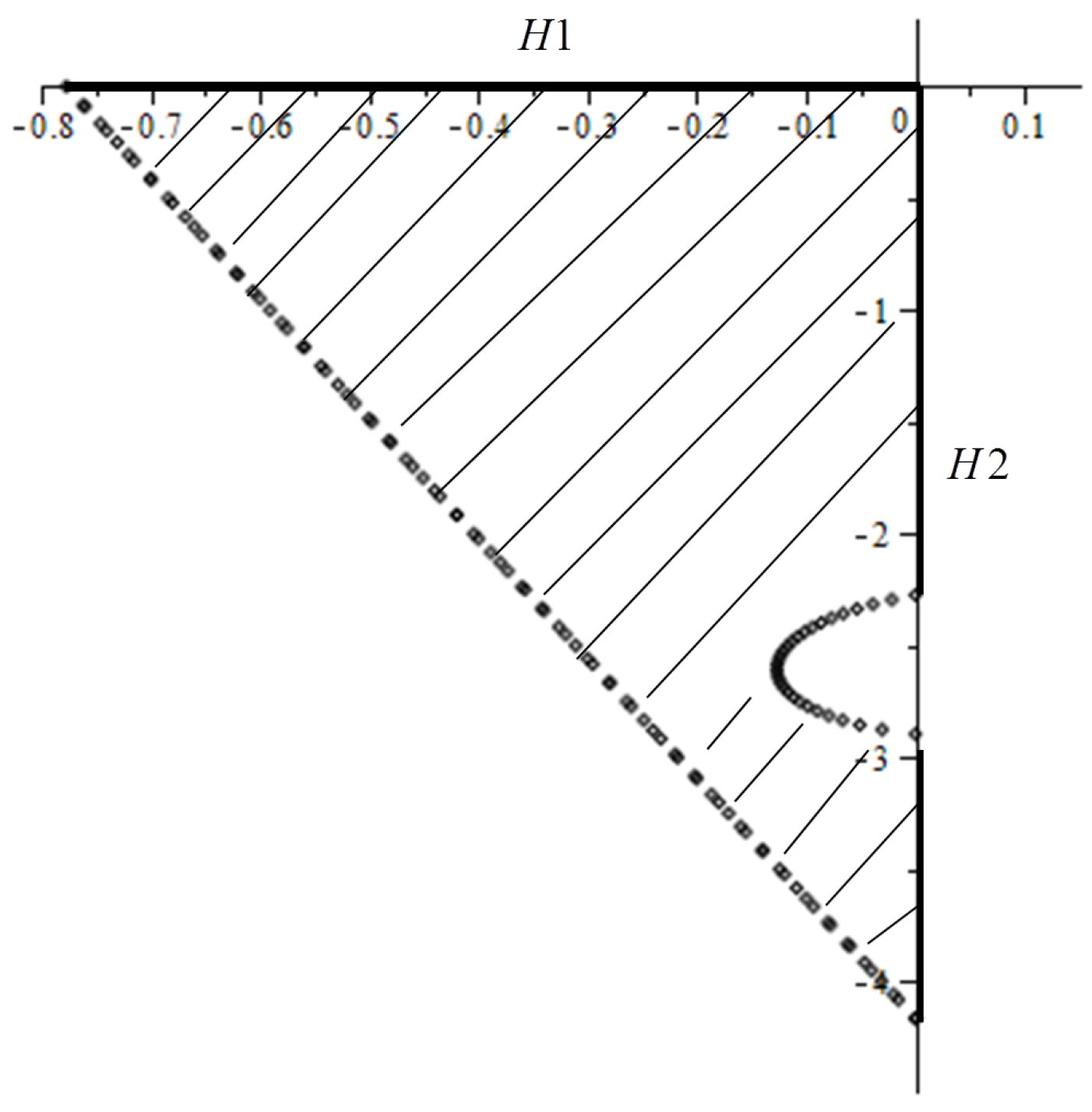
The stability region of the 2PDD6 method is plotted using the coordinate points determined by inserting t in Equation (22) with the values of $1,-1$ and $e^{i\theta }$ for $0\le \theta \le 2\pi$. Replacing $t=e^{i\theta }$ will result in a complex equation. Then, both the real and imaginary parts will be solved simultaneously. Figure 2 illustrates the stability region for the proposed 2PDD6 method in the H1-H2 plane. This enclosed region is traced by finding the region that satisfies $\left|t\right|<1$.

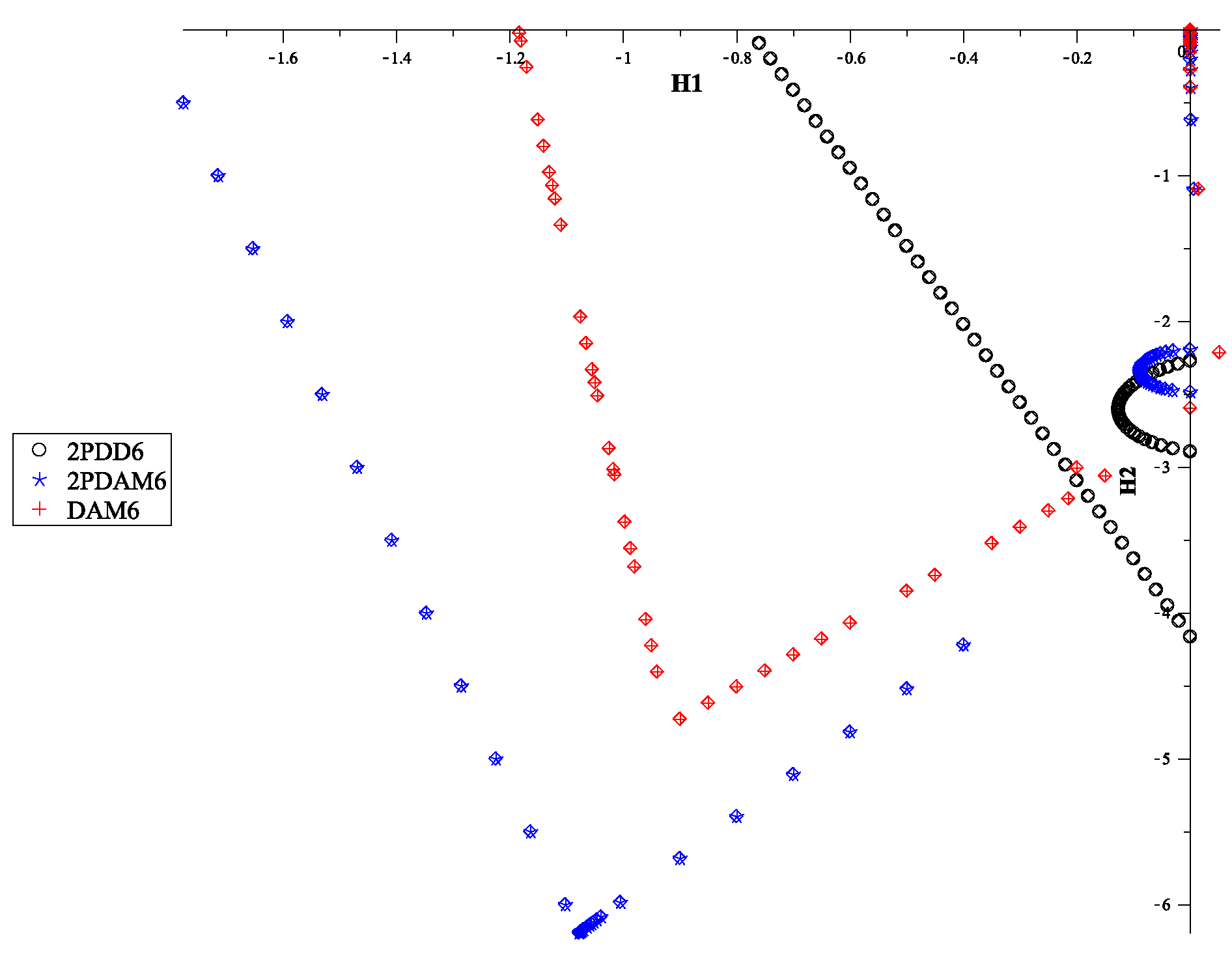
Transparent comparison are plotted in Figure 3 to examine the stability regions between the proposed 2PDD6 method, the fully implicit 2PDAM6 method of order six by Phang et al. [6], and the DAM6 method of order six by Majid et al. [13]. As observed, the stability region of the 2PDD6 method is smaller compared to the other existing methods. It was proven by the study conducted by Majid [18] that the stability region for the fully implicit method is wider than the diagonal method. Nevertheless, we can expect that the performance analysis of the proposed method is at least comparable with the existing methods and has the ability to preserve the accuracy because all the methods possess the same order.

4. Implementation

Our interest is to apply the shooting technique to solve Equation (1) together with the 2PDD6 method proposed in this study. The systematic procedure lies as a ground idea in the shooting methods starting by converting the BVPs into a couple of initial value problems (IVPs). Then, the appropriate initial values are chosen or guessed so that the approximate solutions are satisfied as close as possible to the required right boundary conditions either concomitantly in the Type 1 or Type 2 form.

For Type 1, the boundary conditions in Equation (4) will be transformed to the initial conditions with initial estimates, $s_0$, as follows:

$$y\left(a\right)=\alpha ,y^{\prime }\left(a\right)=s_0,$$

(23)

whereas for Type 2, the given boundary conditions translate to:

$$y\left(a\right)=s_0,y^{\prime }\left(a\right)=V_1-Cy\left(a\right),$$

(24)

where $V_1=\frac{\alpha }{C_1}$ and $C=\frac{C_2}{C_1}$.

The specific steps for producing a numerical solution to the BVPs of either imposing Type 1 or Type 2 by the shooting method are given as follows

• Set $s_0$, and compute the numerical solution using the 2PDD6 formulae.
• At $x_N=b$, verify if $Y_N$ nearly satisfies $\beta$ or not within the specified set of tolerance, TOL.
  $Y_N$ for Type 1 and Type 2 are represented as $Y_N=C_3{y}^{\prime }\left(b\right)+C_{4}y\left(b\right)\cong \beta$ and $Y_N=y^{\prime }\left(b\right)\cong \beta$, respectively.
• If the prescribed stopping condition, $\left|Y_N-\beta \right|\le$ TOL, is satisfied, then the required numerical solution is achieved. Otherwise, set the new guessing value, $s_n$, for $n=1,2,\dots$ using Steffensen’s method. The entire process is repeated.

This iterative process is continued by revising the new estimate of $s_n$ for $n=1,2,\dots$ using Steffensen’s approach as follows:

$$\begin{array}{c}\hfill s_n=s_{n-1}-\left[\frac{{\left(F\left(s_{n-1}\right)\right)}^2}{F\left(s_{n-1}+F\left(s_{n-1}\right)\right)-F\left(s_{n-1}\right)}\right]\end{array}$$

(25)

where for Type 1: $F\left(s_{n-1}\right)=C_3{y}^{\prime }(b,s_{n-1})+C_{4}y(b,s_{n-1})-\beta$ and for Type 2: $F\left(s_{n-1}\right)=y^{\prime }(b,s_{n-1})-\beta$, until a satisfactory stopping criterion is achieved.

The previous initial guesses, the associated $Y_N$, and the required right boundary condition will be involved in the calculation to generate the new $s_n$. The value for $s_0$ chosen in this study was based on the consideration in Burden and Faires [19] and Roberts [20] for $s_0=\frac{\beta -\alpha }{b-a}$ and $s_0=0$, respectively. The details approach on our method is presented in Algorithm 1.

Algorithm 1. The 2PDD6 method.
Step 1:	Set TOL, step size, h, and initial estimate, $s_0.$
Step 2:	Calculate $x_n=x_0+nh$ for $n=1,2,3,4$.
Step 3:	For $n=1,2,3,4$, calculate the starting values using the one step method.
Step 4:	For $n=4$, and $i=1$ to 2, do
	$x_{i+2}=x_n+ih$, and compute $y_{n+i}$, $y_{n+i}^{\prime }$ and $F_{n+i}$ using the predictor and corrector formulas
	with PE(CE)${}^r$ modes where $r=1,2,\dots$ until convergence.
	The calculation of the corrector formula as in Equations (13) to (14) involved in the convergence test.
Step 5:	For $i=0,1,\dots ,4$, set
	$x_i=x_{i+2}$, $y_i=y_{i+2}$, $y_i^{\prime }=y_{i+2}^{\prime }$, $F_i=F_{i+2}$.
Step 6:	If $x_4<b$, then repeat Step 4. Else, go to Step 7.
Step 7:	At $x_4=b$, verify the stopping condition, $|Y_N-\beta |\le TOL$. If satisfied, then go to Step 9.
	Else, continue Step 8.
Step 8:	Correct a new set of guessing values, $s_n$, for $n=1,2,3\dots$ using the formula in Equation (25).
	Repeat Step 2.
Step 9:	Compute the results. Complete.

The accuracy of the method is defined by the magnitude of the numerical error that is obtained using the following formula:

$$\left|\frac{y\left(x_i\right)-y_i}{A+B\left(y\left(x_i\right)\right)}\right|.$$

At the same time, our algorithm also involves the convergence test for a better accuracy result, and the respective formula is given by:

$$\left|\frac{y_{n+1}^r-y_{n+1}^{r-1}}{A+B\left(y_{n+1}^r\right)}\right|<0.1\times TOL.$$

The values assigned for A and B correspond to three different types of error, which are the absolute error test for $A=1,B=0$, the mixed error test for $A=1,B=1$, and the relative error test for $A=0,B=1$. The coding was written using the C language, and the computational procedure was computed using the Code::Blocks 16.01 platform.

5. Results and Discussion

This section is devoted to demonstrating the accuracy, efficiency, and applicability of the proposed 2PDD6 method in solving four numerically tested problems in the form of Equation (1) associated with either Type 1 or Type 2 boundary conditions. Problems 1 to 3 used the absolute error test, while Problem 4 used the mixed error test. Tolerance, $TOL={10}^{-5}$, was set as the stopping criterion throughout the calculation in order to obtain the required solutions.

Problem 1.

Given differential equations:

$$y^{″}\left(x\right)=\frac{1}{x^2}\left(2-3x{y}^{\prime }\left(x\right)\right),1\le x\le 3$$

with Type 1: $y\left(1\right)=4$ and $y^{\prime }\left(3\right)+y\left(3\right)=0.$

The exact solution is $y\left(x\right)=ln\left(x\right)-\frac{1}{2x^2}\left(-9-\frac{27}{13}ln\left(3\right)\right)-\frac{1}{2}-\frac{27}{26}ln\left(3\right).$

Problem 2.

Given differential equations:

$$y^{″}\left(x\right)=\frac{1}{1+x^2}(-2x{y}^{\prime }\left(x\right)+2)+y\left(x\right)-log(1+x^2),0\le x\le 1$$

with Type 1: $y\left(0\right)=0$ and $y^{\prime }\left(1\right)+y\left(1\right)=1+log\left(2\right).$ The exact solution is $y\left(x\right)=log(1+x^2).$

Problem 3.

Given differential equations:

$$y^{″}\left(x\right)=-exp(-2y\left(x\right)),0\le x\le 1$$

with Type 2: $y^{\prime }\left(0\right)+y\left(0\right)=1$ and $y^{\prime }\left(1\right)=\frac{1}{2}.$ The exact solution is $y\left(x\right)=ln(1+x).$

Problem 4.

Given differential equations:

$$y^{″}\left(x\right)=y^2\left(x\right)+2{\pi }^{2}cos\left(2\pi x\right)-si{n}^4\left(\pi x\right),0\le x\le 1$$

with Type 2: $y^{\prime }\left(0\right)+y\left(0\right)=0$ and $y^{\prime }\left(1\right)=0.$ The exact solution is $y\left(x\right)=si{n}^2\left(\pi x\right).$

For a comparable comparison, the numerical results generated by the 2PDD6 method were compared with the results generated by the DAM6 and 2PDAM6 methods, where all the methods satisfied the method of order six. However, the 2PDAM6 method fulfilled the fully implicit features. In addition to that, all the numerical results in

Table 1. Results for solving Test Problem 1.

Method	h	MAXER	AVERR	TStep	TFC	TG	Time
DAM6	0.10	1.0564(−4)	5.5715(−5)	20	65	2	0.459
	0.05	4.5582(−6)	2.1032(−6)	40	73	3	0.485
	0.01	3.9852(−9)	1.4829(−9)	200	228	2	0.544
	0.001	2.5269(−13)	1.8016(−13)	2000	2028	2	0.647
2PDAM6	0.10	9.1588(−5)	2.7699(−5)	12	96	3	0.138
	0.05	1.5746(−5)	1.0187(−5)	22	116	3	0.147
	0.01	6.6570(−9)	3.2354(−9)	102	424	2	0.182
	0.001	4.3965(−14)	2.0196(−14)	1002	4024	2	0.478
2PDD6	0.10	2.3596(−4)	1.4009(−4)	12	68	2	0.126
	0.05	6.1990(−6)	3.9173(−6)	22	74	2	0.136
	0.01	3.7837(−9)	1.2019(−9)	102	228	2	0.172
	0.001	2.1760(−13)	1.4017(−13)	1002	2028	2	0.219

,

Table 2. Results for solving Test Problem 2.

Method	h	MAXER	AVERR	TStep	TFC	TG	Time
DAM6	0.10	5.5585(−6)	3.8778(−6)	10	44	2	0.396
	0.05	6.8134(−8)	4.0499(−8)	20	48	2	0.410
	0.01	4.7002(−12)	3.0072(−12)	100	128	2	0.442
	0.001	1.9984(−15)	6.3048(−16)	1000	1028	2	0.541
2PDAM6	0.10	2.3984(−6)	1.4746(−6)	7	56	2	0.146
	0.05	2.1534(−7)	1.0869(−7)	12	64	2	0.182
	0.01	1.1817(−11)	6.3774(−12)	52	224	2	0.203
	0.001	1.8874(−15)	6.7210(−16)	502	2014	2	0.497
2PDD6	0.10	1.7657(−6)	1.2702(−6)	7	44	2	0.120
	0.05	1.0605(−8)	4.7569(−9)	12	48	2	0.141
	0.01	3.4963(−13)	8.8978(−14)	52	128	2	0.156
	0.001	2.3315(−15)	9.3690(−16)	502	1028	2	0.367

,

Table 3. Results for solving Test Problem 3.

Method	h	MAXER	AVERR	TStep	TFC	TG	Time
DAM6	0.10	4.2518(−6)	2.2424(−6)	10	39	1	0.387
	0.05	2.0221(−7)	1.0901(−7)	20	48	1	0.394
	0.01	8.3222(−11)	4.8364(−11)	100	128	1	0.403
	0.001	8.8818(−16)	4.3506(−16)	1000	1028	1	0.449
2PDAM6	0.10	3.3869(−6)	1.9785(−6)	7	48	1	0.125
	0.05	1.7258(−7)	9.8088(−8)	12	64	1	0.139
	0.01	7.8293(−11)	4.6356(−11)	52	224	1	0.143
	0.001	1.9984(−15)	1.0042(−15)	502	2024	1	0.272
2PDD6	0.10	3.0436(−6)	1.9095(−6)	7	40	1	0.111
	0.05	1.4687(−7)	8.9600(−8)	12	48	1	0.125
	0.01	7.5328(−11)	4.5165(−11)	52	128	1	0.135
	0.001	1.9984(−15)	1.0142(−15)	502	1028	1	0.235

and

Table 4. Results for solving Test Problem 4.

Method	h	MAXER	AVERR	TStep	TFC	TG	Time
DAM6	0.10	2.4032(−3)	1.2027(−3)	10	46	3	0.421
	0.05	2.0730(−5)	1.2485(−5)	20	64	2	0.439
	0.01	6.5416(−9)	1.8124(−9)	100	128	1	0.419
	0.001	7.1180(−14)	2.2245(−14)	1000	1028	1	0.442
2PDAM6	0.10	3.5119(−3)	1.7495(−3)	7	56	2	0.143
	0.05	6.4821(−5)	3.2109(−5)	12	92	2	0.185
	0.01	6.5757(−9)	1.9641(−9)	52	224	1	0.215
	0.001	7.3618(−14)	2.3120(−14)	502	2024	1	0.395
2PDD6	0.10	5.1071(−4)	2.7006(−4)	7	46	2	0.137
	0.05	2.7670(−5)	1.4512(−5)	12	64	2	0.162
	0.01	6.4668(−9)	2.0067(−9)	52	128	1	0.172
	0.001	7.2182(−14)	2.2759(−14)	502	1028	1	0.364

were computed using the same shooting strategy as discussed in Section Four.

As we can see in Table 1, at $h=0.05$, 2PDD6 converged faster than the other methods because 2PDD6 acquired the least initial estimates, which resulted in fewer iterations. In solving Problem 2, at $h=0.05$ and $h=0.01$, 2PDD6 obtained better accuracy results than the other methods as depicted in Table 2. This reflects that 2PDD6 achieved the smallest magnitude of error when comparing the numerical outputs with the true solution. The accuracy and total guessing values were comparable between 2PDD6 and the other methods when solving Problem 3 at all step sizes, except for $h=0.001$; the accuracy of DAM6 was slightly better than 2PDD6, as presented in Table 3. Nevertheless, 2PDD6 dominated other methods in terms of timing. Table 4 demonstrates that 2PDD6 obtained superiority in terms of accuracy compared to the DAM6 and 2PDAM6 methods at $h=0.1$. In addition to that, 2PDD6 acquired one less guessing value than DAM6.

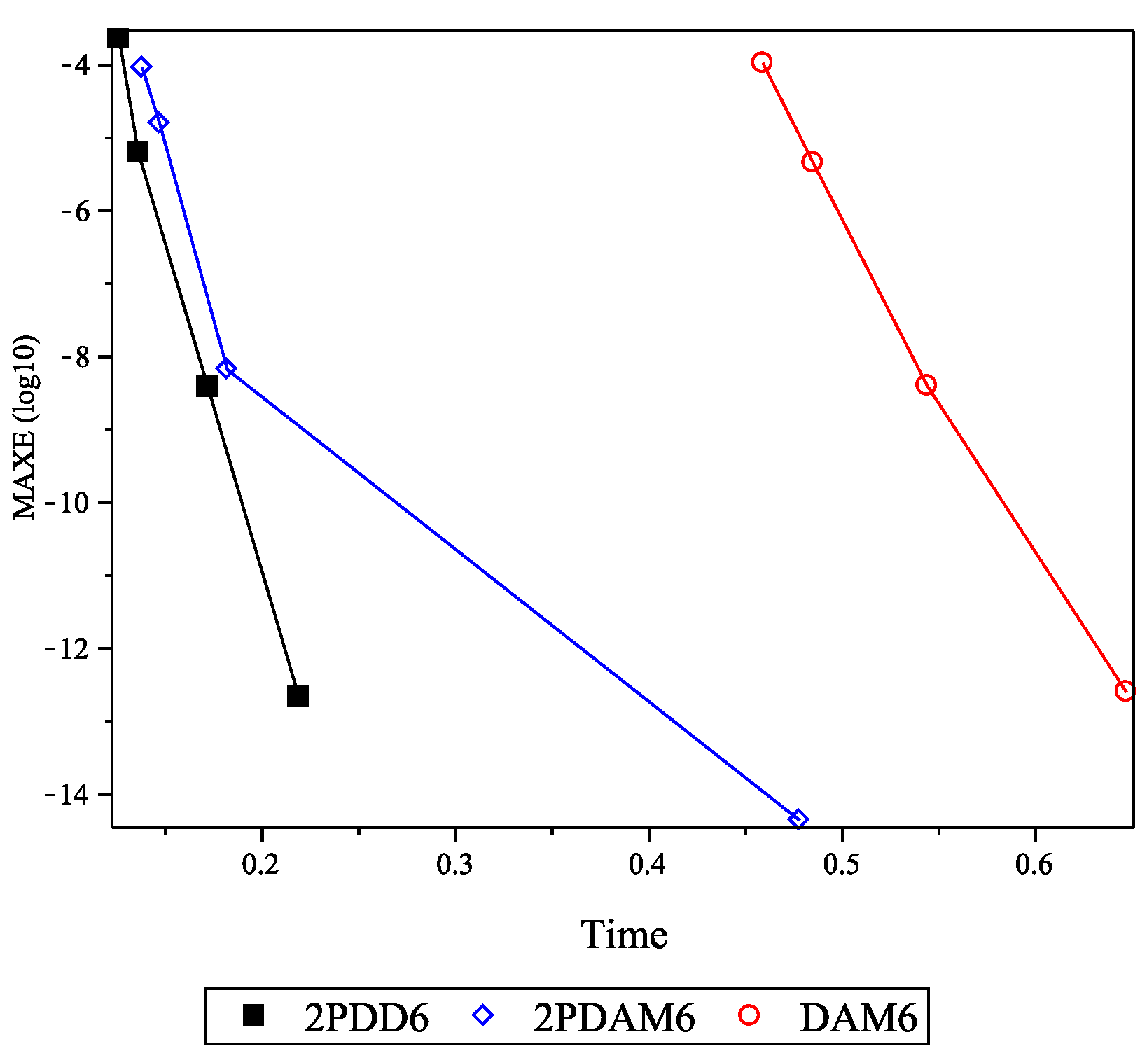
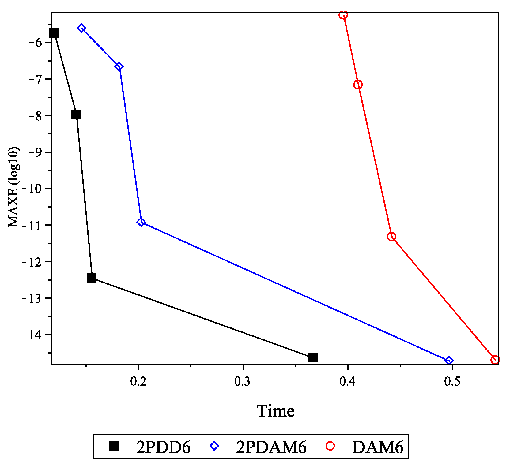
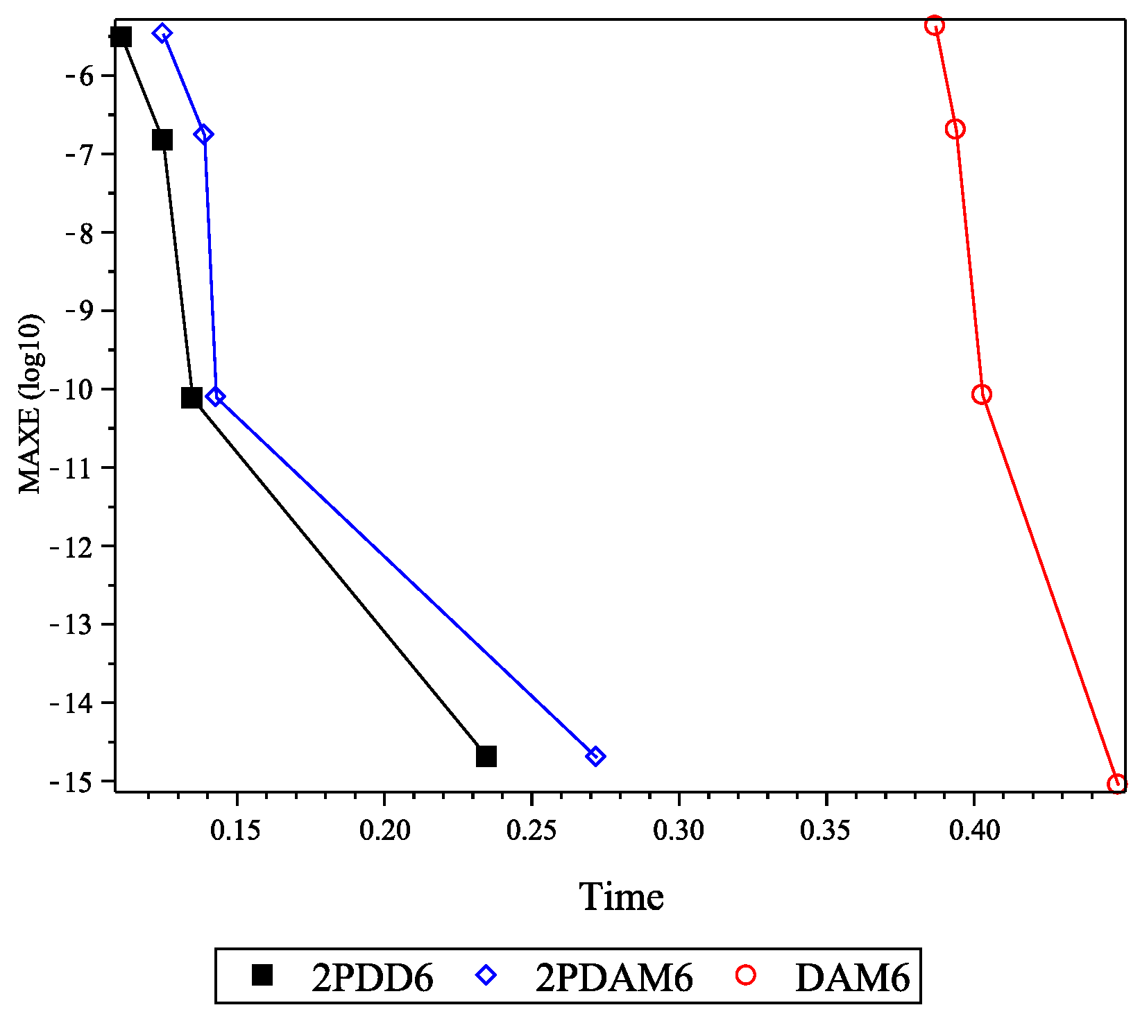
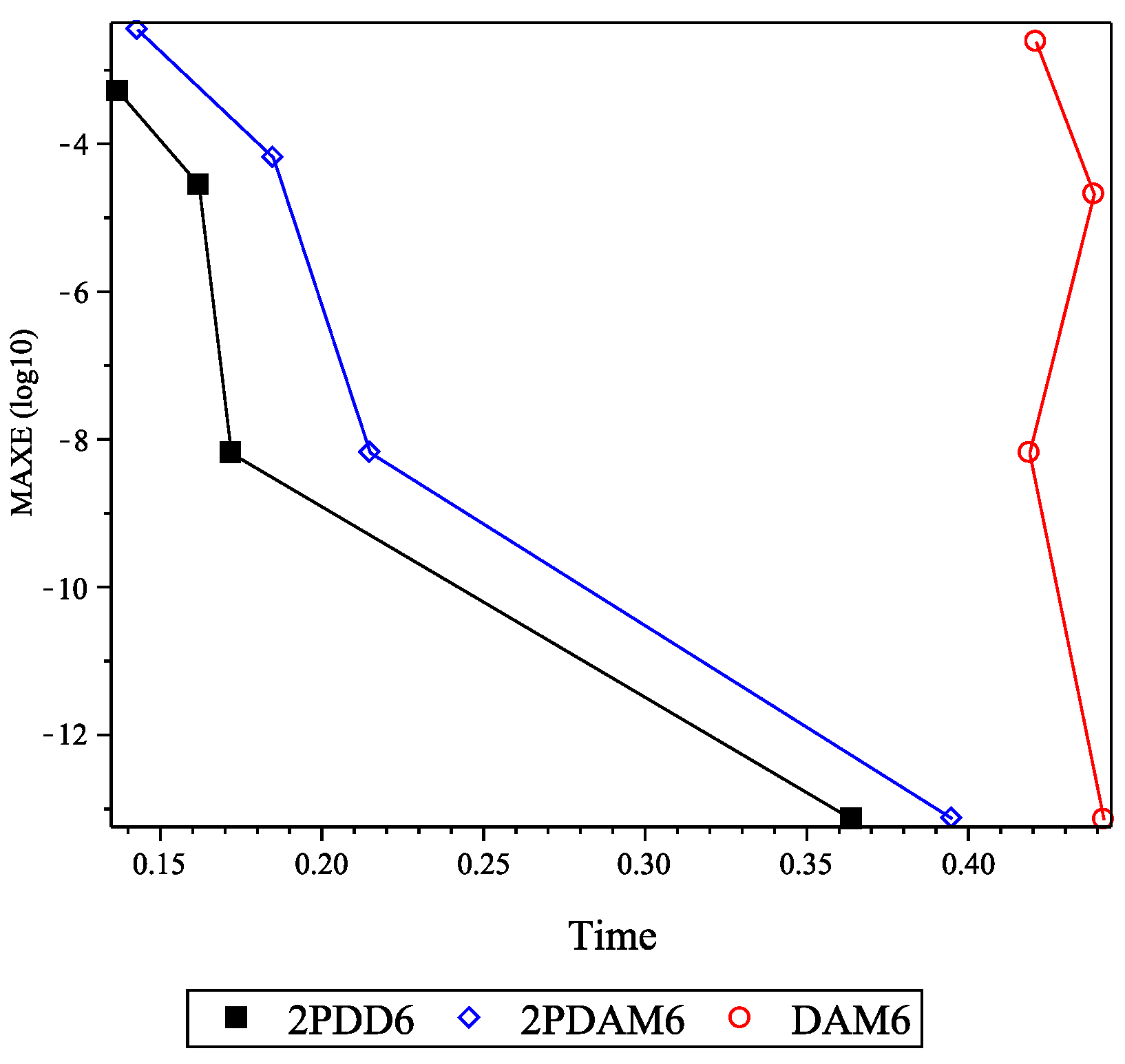
Overall, 2PDD6 reached the end interval much faster than DAM6 because two numerical values were generated at one time in the 2PDD6 scheme. This was expected since the total steps taken by 2PDD6 were less than DAM6 by almost half. Beside that, 2PDD6 accumulated less total function calls than 2PDAM6 because diagonal formulas are inexpensive in terms of function evaluations than full formulas. These performances signify that 2PDD6 required less consumption of time when solving all the tested problems, as tabulated in Table 1, Table 2, Table 3 and Table 4. The performance graphs in Figure 4, Figure 5, Figure 6 and Figure 7 visualize the best performances of the 2PDD6 method subject to accuracy and execution speed for a clear comparison with the 2PDAM6 and DAM6 methods.

6. Conclusions

We conclude that the proposed two point diagonally block method of order six was more adequate and competitive to preserve the accuracy, as well as being faster in executing the numerical results when compared to the existing method for directly solving the second order BVPs subject to Type 1 and Type 2 boundary conditions. Therefore, we recommend our method as an alternative iterative solver that has the ability to reduce the operational cost of the process while computing a trustworthy numerical output.

References

1. Atkinson, K.; Han, W.; Stewart, D.E. Numerical Solution of Ordinary Differential Equations; John Wiley & Sons, Inc.: Hoboken, NJ, USA, 2009; p. 195. [Google Scholar]
2. Cuomo, S.; Marasco, A. A numerical approach to nonlinear two-point boundary value problems for ODEs. Comput. Math. Appl. 2008, 55, 2476–2489. [Google Scholar] [CrossRef] [Green Version]
3. Duan, J.-S.; Rach, R.; Wazwaz, A.M.; Chaolu, T.; Wang, Z. A new modified Adomian decomposition method and its multistage form for solving nonlinear boundary value problems with Robin boundary conditions. Appl. Math. Model. 2013, 37, 8687–8708. [Google Scholar] [CrossRef]
4. Anulo, A.A.; Kibret, A.S.; Gonfa, G.G.; Negassa, A.D. Numerical solution of linear second order ordinary differential equations with mixed boundary conditions by Galerkin method. Math. Comput. Sci. 2017, 2, 66–78. [Google Scholar] [CrossRef]
5. Awoyemi, D.O.; Adebile, E.A.; Adesanya, A.O.; Anake, T.A. Modified block method for the direct solution of second order ordinary differential equations. Int. J. Appl. Math. Comput. 2011, 3, 181–188. [Google Scholar]
6. Phang, P.S.; Majid, Z.A.; Suleiman, M. On the solution of two point boundary value problems with two point direct method. Int. J. Mod. Phys. Conf. Ser. 2012, 9, 566–573. [Google Scholar] [CrossRef]
7. Waeleh, N.; Majid, Z.A. Numerical algorithm of block method for general second order ODEs using variable step size. Sains Malays. 2017, 46, 817–824. [Google Scholar] [CrossRef]
8. Nasir, N.M.; Majid, Z.A.; Ismail, F.; Bachok, N. Diagonal block method for solving two-point boundary value problems with Robin boundary conditions. Math. Prob. Eng. 2018, 2018, 2056834. [Google Scholar]
9. Nasir, N.M.; Majid, Z.A.; Ismail, F.; Bachok, N. Two point diagonally block method for solving boundary value problems with Robin boundary conditions. Malays. J. Math. Sci. 2019, 13, 1–14. [Google Scholar]
10. Ramos, H.; Rufai, M.A. A third-derivative two-step block Falkner-type method for solving general second-order boundary-value systems. Math. Comput. Simul. 2019, 165, 139–155. [Google Scholar] [CrossRef]
11. Ramos, H.; Rufai, M.A. Numerical solution of boundary value problems by using an optimized two-step block method. Numer. Algorithms 2019, 1–23. [Google Scholar] [CrossRef]
12. Ha, S.N. A nonlinear shooting method for two-point boundary value problems. Comput. Math. Appl. 2001, 42, 1411–1420. [Google Scholar] [CrossRef] [Green Version]
13. Majid, Z.A.; Phang, P.S.; Suleiman, M. Solving directly two point non linear boundary value problems using direct Adams–Moulton method. J. Math. Stat. 2011, 7, 124–128. [Google Scholar] [CrossRef]
14. Lambert, J.D. Computational Methods in Ordinary Differential Equations; John Wiley & Sons Ltd.: Great Britain, UK, 1973; pp. 252–254. [Google Scholar]
15. Fatunla, S.O. Block methods for second order ODEs. Int. J. Comput. Math. 1991, 41, 55–63. [Google Scholar] [CrossRef]
16. Ramos, H.; Kalogiratou, Z.; Monovasilis, T.; Simos, T.E. An optimized two-step hybrid block method for solving general second order initial-value problems. Numer. Algorithms 2016, 72, 1089–1102. [Google Scholar] [CrossRef]
17. Ackleh, A.S.; Allen, E.J.; Kearfott, R.B.; Seshaiyer, P. Classical and Modern Numerical Analysis: Theory, Methods and Practice; CRC Press: London, UK, 2009; pp. 412–414. [Google Scholar]
18. Majid, Z.A. Parallel Block Methods for Solving Ordinary Differential Equations. Ph.D. Thesis, Universiti Putra Malaysia, Selangor, Malaysia, 2004. [Google Scholar]
19. Burden, R.L.; Faires, J.D. Numerical Analysis, 9th ed.; Brooks/Cole, Cengage Learning: Boston, MA, USA, 2011; p. 681. [Google Scholar]
20. Roberts, C.E. Ordinary Differential Equations: A Computational Approach; Prentice-Hall, Inc.: Englewood Cliffs, NJ, USA, 1979; pp. 353–354. [Google Scholar]
Figure 1. Two point block method.
Mathematics 07 01075 g001
Figure 2. Stability region of the proposed direct block method of order six (2PDD6) method.
Mathematics 07 01075 g002
Figure 3. Comparison of the stability regions between 2PDD6, 2PDAM6, and DAM6.
Mathematics 07 01075 g003
Figure 4. Performance graphs of time vs. log MAXE for Problem 1.
Mathematics 07 01075 g004
Figure 5. Performance graphs of time vs. log MAXE for Problem 2.
Mathematics 07 01075 g005
Figure 6. Performance graphs of time vs. log MAXE for Problem 3.
Mathematics 07 01075 g006
Figure 7. Performance graphs of time vs. log MAXE for Problem 4.
Mathematics 07 01075 g007