Direct Integration of Boundary Value Problems Using the Block Method via the Shooting Technique Combined with Steffensen’s Strategy


Abstract
1. Introduction
- ,
- for some constant, ,
- For the boundary conditions of Equation (2), assume:
2. Methodology
3. Analysis of the Block Method
3.1. Order and Error Constant
3.2. Stability
- all roots, , of satisfy ,
- for those roots with , the multiplicity must not exceed two.
3.3. Consistency and Convergence of the Method
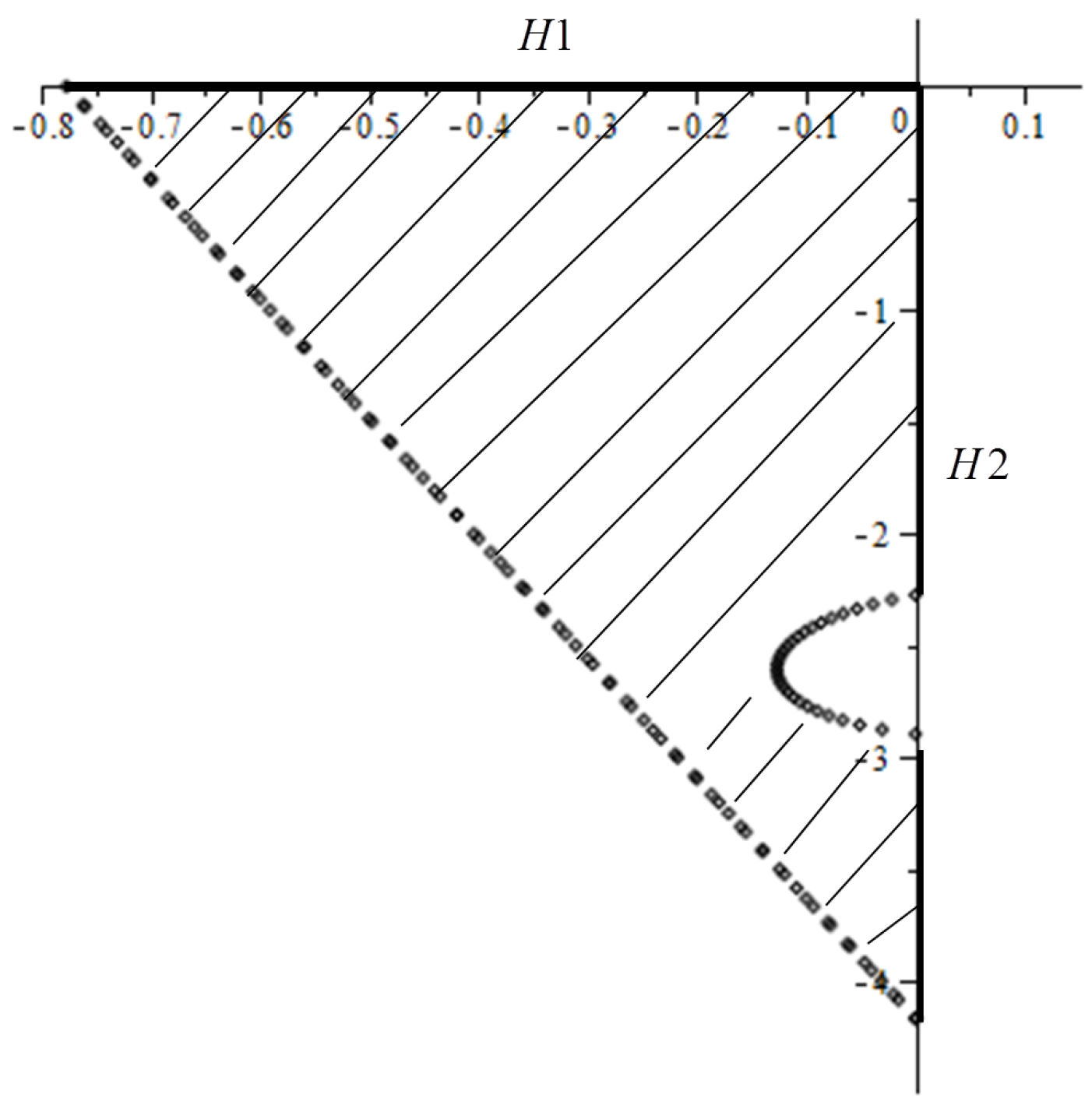
3.4. Stability Analysis
4. Implementation
- Set , and compute the numerical solution using the 2PDD6 formulae.
- At , verify if nearly satisfies or not within the specified set of tolerance, TOL.for Type 1 and Type 2 are represented as and , respectively.
- If the prescribed stopping condition, TOL, is satisfied, then the required numerical solution is achieved. Otherwise, set the new guessing value, , for using Steffensen’s method. The entire process is repeated.
| Algorithm 1. The 2PDD6 method. | |
| Step 1: | Set TOL, step size, h, and initial estimate, |
| Step 2: | Calculate for . |
| Step 3: | For , calculate the starting values using the one step method. |
| Step 4: | For , and to 2, do |
| , and compute , and using the predictor and corrector formulas | |
| with PE(CE) modes where until convergence. | |
| The calculation of the corrector formula as in Equations (13) to (14) involved in the convergence test. | |
| Step 5: | For , set |
| , , , . | |
| Step 6: | If , then repeat Step 4. Else, go to Step 7. |
| Step 7: | At , verify the stopping condition, . If satisfied, then go to Step 9. |
| Else, continue Step 8. | |
| Step 8: | Correct a new set of guessing values, , for using the formula in Equation (25). |
| Repeat Step 2. | |
| Step 9: | Compute the results. Complete. |
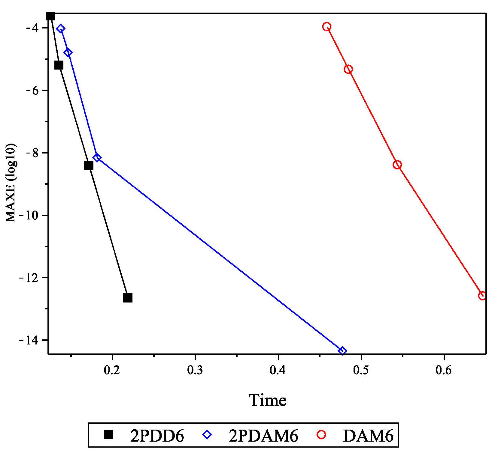
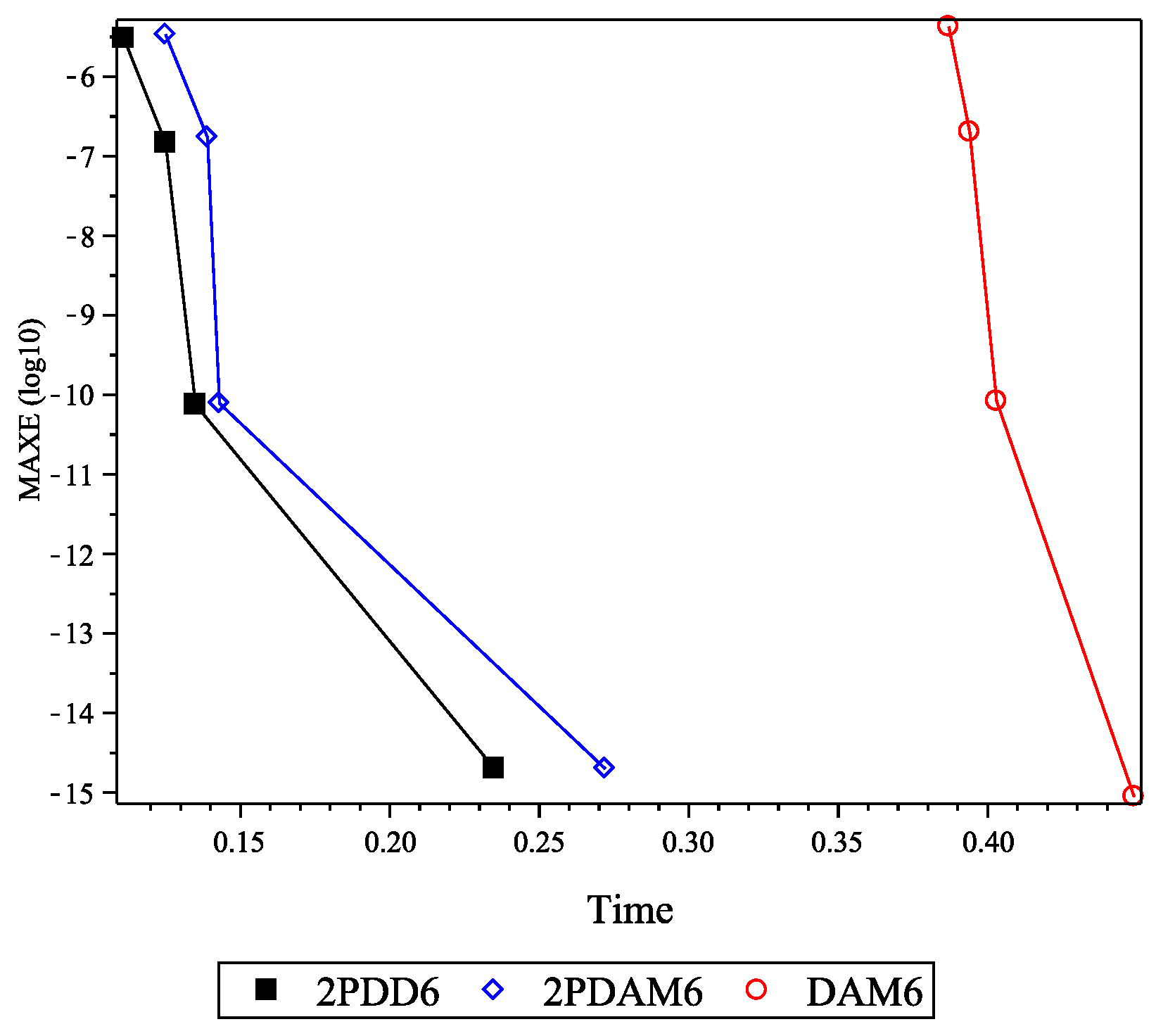
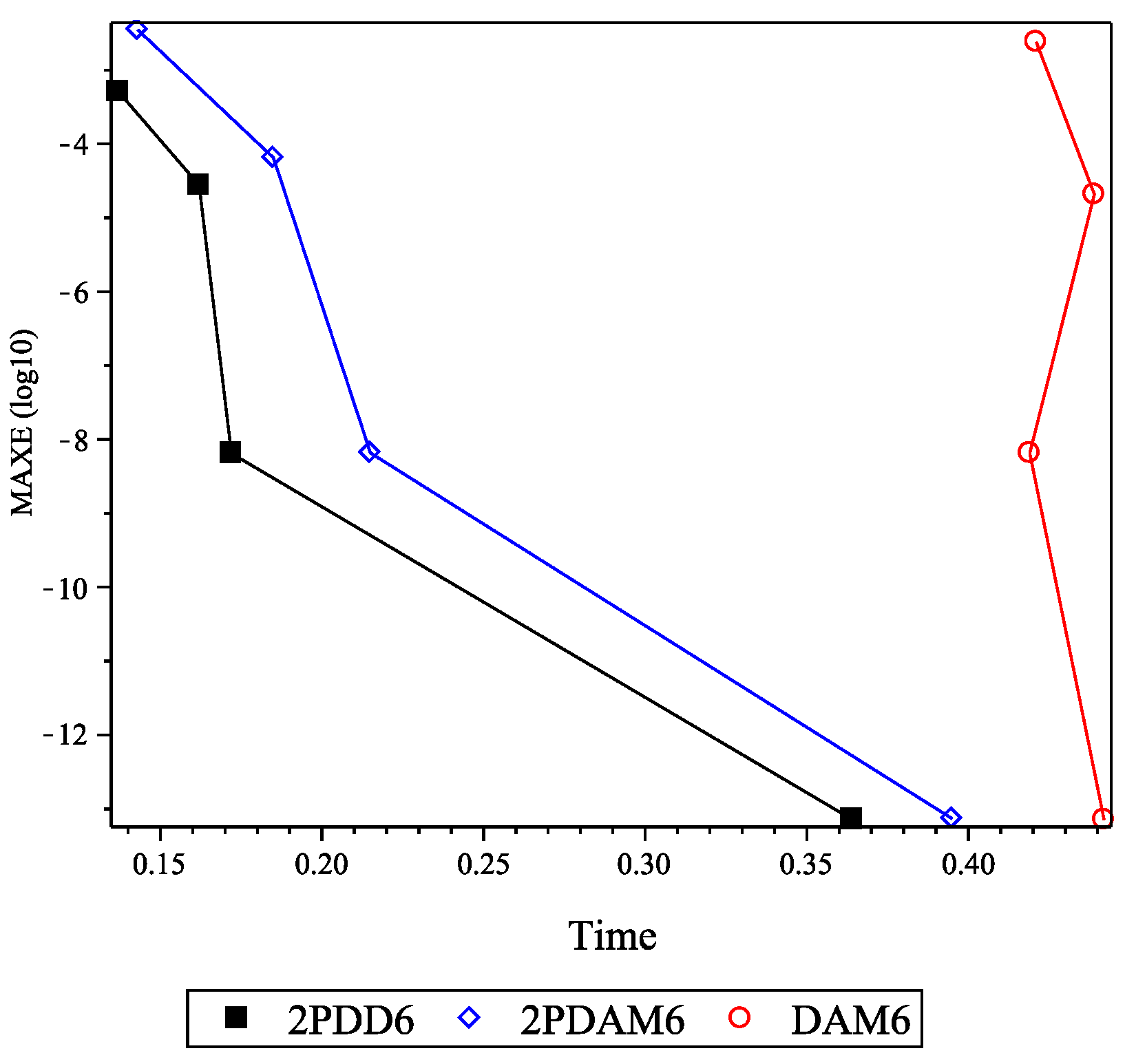
5. Results and Discussion
6. Conclusions
Author Contributions
Funding
Acknowledgments
Conflicts of Interest
Abbreviations
| MAXER: | Maximum error |
| AVERR: | Average error |
| h: | Step size |
| TStep: | Total steps taken at the last iteration |
| TFC: | Total function call at the last iteration |
| TG: | Total number of guesses |
| Time: | Execution time in seconds |
| 2PDD6: | Direct two point diagonal block method of order six proposed in this study |
| 2PDAM6: | Direct two step Adams–Moulton block method of order six as in Phang et al. [6] |
| DAM6: | Direct Adams–Moulton method of order six as in Majid et al. [13] |
References
- Atkinson, K.; Han, W.; Stewart, D.E. Numerical Solution of Ordinary Differential Equations; John Wiley & Sons, Inc.: Hoboken, NJ, USA, 2009; p. 195. [Google Scholar]
- Cuomo, S.; Marasco, A. A numerical approach to nonlinear two-point boundary value problems for ODEs. Comput. Math. Appl. 2008, 55, 2476–2489. [Google Scholar] [CrossRef]
- Duan, J.-S.; Rach, R.; Wazwaz, A.M.; Chaolu, T.; Wang, Z. A new modified Adomian decomposition method and its multistage form for solving nonlinear boundary value problems with Robin boundary conditions. Appl. Math. Model. 2013, 37, 8687–8708. [Google Scholar] [CrossRef]
- Anulo, A.A.; Kibret, A.S.; Gonfa, G.G.; Negassa, A.D. Numerical solution of linear second order ordinary differential equations with mixed boundary conditions by Galerkin method. Math. Comput. Sci. 2017, 2, 66–78. [Google Scholar] [CrossRef]
- Awoyemi, D.O.; Adebile, E.A.; Adesanya, A.O.; Anake, T.A. Modified block method for the direct solution of second order ordinary differential equations. Int. J. Appl. Math. Comput. 2011, 3, 181–188. [Google Scholar]
- Phang, P.S.; Majid, Z.A.; Suleiman, M. On the solution of two point boundary value problems with two point direct method. Int. J. Mod. Phys. Conf. Ser. 2012, 9, 566–573. [Google Scholar] [CrossRef]
- Waeleh, N.; Majid, Z.A. Numerical algorithm of block method for general second order ODEs using variable step size. Sains Malays. 2017, 46, 817–824. [Google Scholar] [CrossRef]
- Nasir, N.M.; Majid, Z.A.; Ismail, F.; Bachok, N. Diagonal block method for solving two-point boundary value problems with Robin boundary conditions. Math. Prob. Eng. 2018, 2018, 2056834. [Google Scholar]
- Nasir, N.M.; Majid, Z.A.; Ismail, F.; Bachok, N. Two point diagonally block method for solving boundary value problems with Robin boundary conditions. Malays. J. Math. Sci. 2019, 13, 1–14. [Google Scholar]
- Ramos, H.; Rufai, M.A. A third-derivative two-step block Falkner-type method for solving general second-order boundary-value systems. Math. Comput. Simul. 2019, 165, 139–155. [Google Scholar] [CrossRef]
- Ramos, H.; Rufai, M.A. Numerical solution of boundary value problems by using an optimized two-step block method. Numer. Algorithms 2019, 1–23. [Google Scholar] [CrossRef]
- Ha, S.N. A nonlinear shooting method for two-point boundary value problems. Comput. Math. Appl. 2001, 42, 1411–1420. [Google Scholar] [CrossRef]
- Majid, Z.A.; Phang, P.S.; Suleiman, M. Solving directly two point non linear boundary value problems using direct Adams–Moulton method. J. Math. Stat. 2011, 7, 124–128. [Google Scholar] [CrossRef][Green Version]
- Lambert, J.D. Computational Methods in Ordinary Differential Equations; John Wiley & Sons Ltd.: Great Britain, UK, 1973; pp. 252–254. [Google Scholar]
- Fatunla, S.O. Block methods for second order ODEs. Int. J. Comput. Math. 1991, 41, 55–63. [Google Scholar] [CrossRef]
- Ramos, H.; Kalogiratou, Z.; Monovasilis, T.; Simos, T.E. An optimized two-step hybrid block method for solving general second order initial-value problems. Numer. Algorithms 2016, 72, 1089–1102. [Google Scholar] [CrossRef]
- Ackleh, A.S.; Allen, E.J.; Kearfott, R.B.; Seshaiyer, P. Classical and Modern Numerical Analysis: Theory, Methods and Practice; CRC Press: London, UK, 2009; pp. 412–414. [Google Scholar]
- Majid, Z.A. Parallel Block Methods for Solving Ordinary Differential Equations. Ph.D. Thesis, Universiti Putra Malaysia, Selangor, Malaysia, 2004. [Google Scholar]
- Burden, R.L.; Faires, J.D. Numerical Analysis, 9th ed.; Brooks/Cole, Cengage Learning: Boston, MA, USA, 2011; p. 681. [Google Scholar]
- Roberts, C.E. Ordinary Differential Equations: A Computational Approach; Prentice-Hall, Inc.: Englewood Cliffs, NJ, USA, 1979; pp. 353–354. [Google Scholar]


| Method | h | MAXER | AVERR | TStep | TFC | TG | Time |
|---|---|---|---|---|---|---|---|
| DAM6 | 0.10 | 1.0564(−4) | 5.5715(−5) | 20 | 65 | 2 | 0.459 |
| 0.05 | 4.5582(−6) | 2.1032(−6) | 40 | 73 | 3 | 0.485 | |
| 0.01 | 3.9852(−9) | 1.4829(−9) | 200 | 228 | 2 | 0.544 | |
| 0.001 | 2.5269(−13) | 1.8016(−13) | 2000 | 2028 | 2 | 0.647 | |
| 2PDAM6 | 0.10 | 9.1588(−5) | 2.7699(−5) | 12 | 96 | 3 | 0.138 |
| 0.05 | 1.5746(−5) | 1.0187(−5) | 22 | 116 | 3 | 0.147 | |
| 0.01 | 6.6570(−9) | 3.2354(−9) | 102 | 424 | 2 | 0.182 | |
| 0.001 | 4.3965(−14) | 2.0196(−14) | 1002 | 4024 | 2 | 0.478 | |
| 2PDD6 | 0.10 | 2.3596(−4) | 1.4009(−4) | 12 | 68 | 2 | 0.126 |
| 0.05 | 6.1990(−6) | 3.9173(−6) | 22 | 74 | 2 | 0.136 | |
| 0.01 | 3.7837(−9) | 1.2019(−9) | 102 | 228 | 2 | 0.172 | |
| 0.001 | 2.1760(−13) | 1.4017(−13) | 1002 | 2028 | 2 | 0.219 |
| Method | h | MAXER | AVERR | TStep | TFC | TG | Time |
|---|---|---|---|---|---|---|---|
| DAM6 | 0.10 | 5.5585(−6) | 3.8778(−6) | 10 | 44 | 2 | 0.396 |
| 0.05 | 6.8134(−8) | 4.0499(−8) | 20 | 48 | 2 | 0.410 | |
| 0.01 | 4.7002(−12) | 3.0072(−12) | 100 | 128 | 2 | 0.442 | |
| 0.001 | 1.9984(−15) | 6.3048(−16) | 1000 | 1028 | 2 | 0.541 | |
| 2PDAM6 | 0.10 | 2.3984(−6) | 1.4746(−6) | 7 | 56 | 2 | 0.146 |
| 0.05 | 2.1534(−7) | 1.0869(−7) | 12 | 64 | 2 | 0.182 | |
| 0.01 | 1.1817(−11) | 6.3774(−12) | 52 | 224 | 2 | 0.203 | |
| 0.001 | 1.8874(−15) | 6.7210(−16) | 502 | 2014 | 2 | 0.497 | |
| 2PDD6 | 0.10 | 1.7657(−6) | 1.2702(−6) | 7 | 44 | 2 | 0.120 |
| 0.05 | 1.0605(−8) | 4.7569(−9) | 12 | 48 | 2 | 0.141 | |
| 0.01 | 3.4963(−13) | 8.8978(−14) | 52 | 128 | 2 | 0.156 | |
| 0.001 | 2.3315(−15) | 9.3690(−16) | 502 | 1028 | 2 | 0.367 |
| Method | h | MAXER | AVERR | TStep | TFC | TG | Time |
|---|---|---|---|---|---|---|---|
| DAM6 | 0.10 | 4.2518(−6) | 2.2424(−6) | 10 | 39 | 1 | 0.387 |
| 0.05 | 2.0221(−7) | 1.0901(−7) | 20 | 48 | 1 | 0.394 | |
| 0.01 | 8.3222(−11) | 4.8364(−11) | 100 | 128 | 1 | 0.403 | |
| 0.001 | 8.8818(−16) | 4.3506(−16) | 1000 | 1028 | 1 | 0.449 | |
| 2PDAM6 | 0.10 | 3.3869(−6) | 1.9785(−6) | 7 | 48 | 1 | 0.125 |
| 0.05 | 1.7258(−7) | 9.8088(−8) | 12 | 64 | 1 | 0.139 | |
| 0.01 | 7.8293(−11) | 4.6356(−11) | 52 | 224 | 1 | 0.143 | |
| 0.001 | 1.9984(−15) | 1.0042(−15) | 502 | 2024 | 1 | 0.272 | |
| 2PDD6 | 0.10 | 3.0436(−6) | 1.9095(−6) | 7 | 40 | 1 | 0.111 |
| 0.05 | 1.4687(−7) | 8.9600(−8) | 12 | 48 | 1 | 0.125 | |
| 0.01 | 7.5328(−11) | 4.5165(−11) | 52 | 128 | 1 | 0.135 | |
| 0.001 | 1.9984(−15) | 1.0142(−15) | 502 | 1028 | 1 | 0.235 |
| Method | h | MAXER | AVERR | TStep | TFC | TG | Time |
|---|---|---|---|---|---|---|---|
| DAM6 | 0.10 | 2.4032(−3) | 1.2027(−3) | 10 | 46 | 3 | 0.421 |
| 0.05 | 2.0730(−5) | 1.2485(−5) | 20 | 64 | 2 | 0.439 | |
| 0.01 | 6.5416(−9) | 1.8124(−9) | 100 | 128 | 1 | 0.419 | |
| 0.001 | 7.1180(−14) | 2.2245(−14) | 1000 | 1028 | 1 | 0.442 | |
| 2PDAM6 | 0.10 | 3.5119(−3) | 1.7495(−3) | 7 | 56 | 2 | 0.143 |
| 0.05 | 6.4821(−5) | 3.2109(−5) | 12 | 92 | 2 | 0.185 | |
| 0.01 | 6.5757(−9) | 1.9641(−9) | 52 | 224 | 1 | 0.215 | |
| 0.001 | 7.3618(−14) | 2.3120(−14) | 502 | 2024 | 1 | 0.395 | |
| 2PDD6 | 0.10 | 5.1071(−4) | 2.7006(−4) | 7 | 46 | 2 | 0.137 |
| 0.05 | 2.7670(−5) | 1.4512(−5) | 12 | 64 | 2 | 0.162 | |
| 0.01 | 6.4668(−9) | 2.0067(−9) | 52 | 128 | 1 | 0.172 | |
| 0.001 | 7.2182(−14) | 2.2759(−14) | 502 | 1028 | 1 | 0.364 |
© 2019 by the authors. Licensee MDPI, Basel, Switzerland. This article is an open access article distributed under the terms and conditions of the Creative Commons Attribution (CC BY) license (http://creativecommons.org/licenses/by/4.0/).
Share and Cite
Mohd Nasir, N.; Abdul Majid, Z.; Ismail, F.; Bachok, N. Direct Integration of Boundary Value Problems Using the Block Method via the Shooting Technique Combined with Steffensen’s Strategy. Mathematics 2019, 7, 1075. https://doi.org/10.3390/math7111075
Mohd Nasir N, Abdul Majid Z, Ismail F, Bachok N. Direct Integration of Boundary Value Problems Using the Block Method via the Shooting Technique Combined with Steffensen’s Strategy. Mathematics. 2019; 7(11):1075. https://doi.org/10.3390/math7111075
Chicago/Turabian StyleMohd Nasir, Nadirah, Zanariah Abdul Majid, Fudziah Ismail, and Norfifah Bachok. 2019. "Direct Integration of Boundary Value Problems Using the Block Method via the Shooting Technique Combined with Steffensen’s Strategy" Mathematics 7, no. 11: 1075. https://doi.org/10.3390/math7111075
APA StyleMohd Nasir, N., Abdul Majid, Z., Ismail, F., & Bachok, N. (2019). Direct Integration of Boundary Value Problems Using the Block Method via the Shooting Technique Combined with Steffensen’s Strategy. Mathematics, 7(11), 1075. https://doi.org/10.3390/math7111075