Fault-Tolerant Path-Embedding of Twisted Hypercube-Like Networks (THLNs)


Abstract
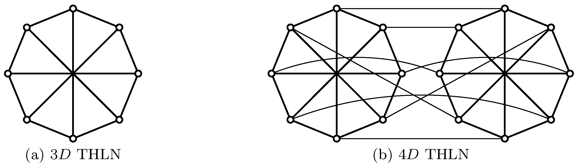
1. Introduction
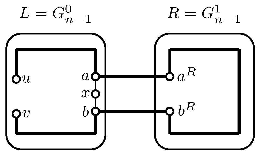
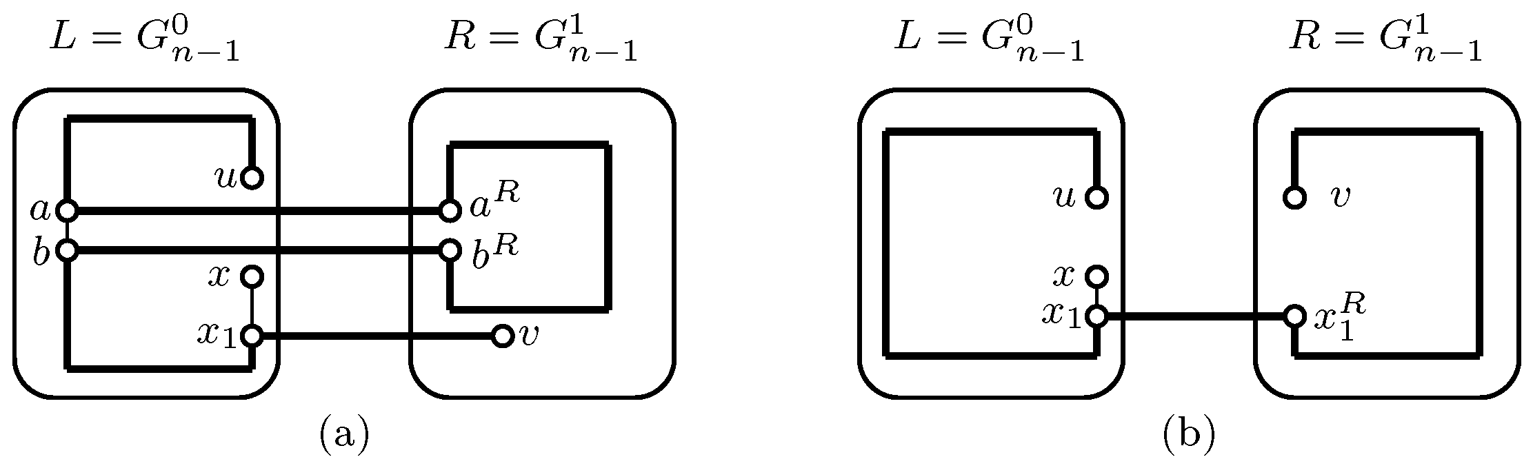
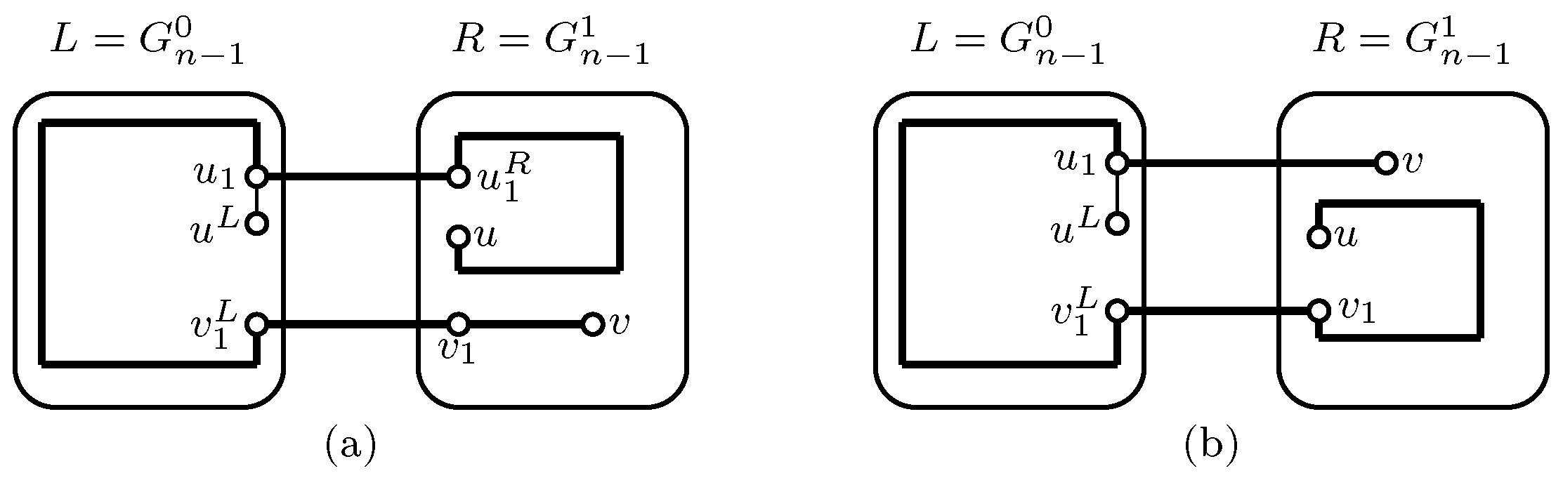
2. Main Result
3. Concluding Remarks
Author Contributions
Funding
Conflicts of Interest
References
- Parhami, B. An Introduction to Parallel Processing: Algorithms and Architectures; Plenum Press: New York, NY, USA, 1999. [Google Scholar]
- Hayes, P.; Mudge, T. Hypercube supercomputers. Proc. IEEE 1989, 77, 1829–1841. [Google Scholar] [CrossRef]
- Andre, F.; Verjus, J. Hypercubes and Distributed Computers; North-Halland: Amsterdam, The Netherlands; New York, NY, USA; Oxford, UK, 1989. [Google Scholar]
- Leighton, F. Introduction to Parallel Algorithms and Architectures: Arrays, Trees, Hypercubes; Morgan Kaufmann Publishers: San Mateo, CA, USA, 1991. [Google Scholar]
- Banks, E. Counting Ten Data Center Network Topologies. 2014. Available online: https://searchdatacenter.techtarget.com.cn/9-20784/ (accessed on 22 October 2014).
- Efe, K. The crossed cube architecture for parallel computation. IEEE Trans. Parallel Distrib. Syst. 1992, 3, 513–524. [Google Scholar] [CrossRef]
- Cull, P.; Larson, S.M. The Möbius cubes. IEEE Trans. Comput. 1995, 44, 647–659. [Google Scholar] [CrossRef]
- Hilbers, P.; Koopman, M.; van de Snepscheut, J. The twisted cube. Lect. Notes Comput. Sci. 1987, 258, 152–159. [Google Scholar]
- Yang, X.; Evans, D.; Megson, G. The locally twisted cubes. Int. J. Comput. Math. 2005, 82, 401–413. [Google Scholar] [CrossRef]
- Xu, J. Topological Structure and Analysis of Interconnection Networks; Kluwer Academic Publishers: Dordrecht, The Netherlands; Boston, MA, USA; London, UK, 2001. [Google Scholar]
- Xu, J. Combinatorial Theory in Networks; Academic Press: Beijing, UK, 2013. [Google Scholar]
- Fan, J.; Lin, X.; Jia, X. Optimal path embedding in crossed cubes. IEEE Trans. Parallel Distrib. Syst. 2005, 16, 1190–1200. [Google Scholar] [CrossRef]
- Fan, J.; Jia, X.; Lin, X. Optimal embeddings of paths with various lengths in twisted cubes. IEEE Trans. Parallel Distrib. Syst. 2007, 18, 511–521. [Google Scholar] [CrossRef]
- Fan, J.; Jia, X. Edge-pancyclicity and path-embeddability of bijective connection graphs. Inf. Sci. 2008, 178, 340–351. [Google Scholar] [CrossRef]
- Bae, M.; Bose, B. Edge disjoint hamiltonian cycles in k-ary n-cubes and hypercubes. IEEE Trans. Comput. 2003, 52, 1271–1284. [Google Scholar] [CrossRef]
- Zhou, D.; Fan, J.; Lin, C.; Zhou, J.; Wang, X. Cycles embedding in exchanged crossed cube. Int. J. Found. Comput. Sci. 2017, 28, 61–76. [Google Scholar] [CrossRef]
- Wagh, M.; Guzide, O. Mapping cycles and trees on wrap-around butterfly graphs. SIAM J. Comput. 2006, 35, 741–765. [Google Scholar] [CrossRef]
- Kulasinghe, P.; Bettayeb, S. Embedding binary trees into crossed cubes. IEEE Trans. Comput. 1995, 44, 923–929. [Google Scholar] [CrossRef]
- Fan, J.; Jia, X. Embedding meshes into crossed cubes. Inform. Sci. 2007, 177, 3151–3160. [Google Scholar] [CrossRef]
- Wang, X.; Fan, J.; Jia, X.; Zhang, S.; Yu, J. Embedding meshes into twisted-cubes. Inf. Sci. 2011, 181, 3085–3099. [Google Scholar] [CrossRef]
- Han, Y.; Fan, J.; Zhang, S.; Yang, J.; Qian, P. Embedding meshes into locally twisted cubes. Inf. Sci. 2010, 180, 3794–3805. [Google Scholar] [CrossRef]
- Wang, H.; Wang, J.; Xu, J. Edge-fault-tolerant bipanconnectivity of hypercubes. Inf. Sci. 2009, 179, 404–409. [Google Scholar] [CrossRef]
- Xu, J.; Ma, M. Survey on path and cycle embedding in some networks. Front. Math. China 2009, 4, 217–252. [Google Scholar] [CrossRef]
- Park, J.; Kim, H.; Lim, H. Fault-Hamiltonicity of hypercube-like interconnection networks. In Proceedings of the IEEE International Parallel and Distributed Processing Symposium, IPDPS, Denver, CO, USA, 4–8 April 2005. [Google Scholar]
- Park, J.; Lim, H.; Kim, H. Panconnectivity and pancyclicity of hypercube-like interconnection networks with faulty elements. Theor. Comput. Sci. 2007, 377, 170–180. [Google Scholar] [CrossRef]
- Zhang, H.; Xu, X.; Guo, J.; Yang, Y. Fault-Tolerant Hamiltonian Connectivity of Twisted Hypercube-Like Networks THLNs. IEEE Access 2018, 6, 74081–74090. [Google Scholar] [CrossRef]
- Zhang, H.; Xu, X.; Yang, Y. (n − 2)-Fault-Tolerant Edge-Pancyclicity of Möbius Cubes MQn. Ars Comb. in press.
- Wang, H.; Wang, J.; Xu, J. Fault-tolerant panconnectivity of augmented cubes. Front. Math. China 2009, 4, 697–719. [Google Scholar] [CrossRef]
- Chan, H.; Chang, J.; Wang, Y.; Horng, S. Geodesic-pancyclicity and fault-tolerant panconnectivity of augmented cubes. Appl. Math. Comput. 2009, 207, 333–339. [Google Scholar] [CrossRef]
- Fan, J.; Lin, X.; Pan, Y.; Jia, X. Optimal fault-tolerant embedding of paths in twisted cubes. J. Parallel Distrib. Comput. 2007, 67, 205–214. [Google Scholar] [CrossRef]
- Chang, J.; Yang, J. Fault-tolerant cycle-embedding in alternating group graphs. Appl. Math. Comput. 2008, 197, 760–767. [Google Scholar] [CrossRef]
- Fu, J. Edge-fault-tolerant vertex-pancyclicity of augmented cubes. Inf. Process Lett. 2010, 110, 439–443. [Google Scholar] [CrossRef]
- Ma, M.; Liu, G.; Xu, J. Fault-tolerant embedding of paths in crossed cubes. Theoret. Comput. Sci. 2008, 407, 110–116. [Google Scholar] [CrossRef]
- Ma, M.; Liu, G.; Pan, X. Path embedding in faulty hypercubes. Appl. Math. Comput. 2007, 192, 233–238. [Google Scholar] [CrossRef]
- Ye, C.; Ma, M.; Wang, W. Fault-tolerant path-embedding in locally twisted cubes. Ars Comb. 2012, 107, 51–63. [Google Scholar]
- Wang, W.; Ma, M.; Xu, J. Fault-tolerant pancyclicity of augmented cubes. Inf. Process Lett. 2007, 103, 52–56. [Google Scholar] [CrossRef]
- Xu, X.; Zhang, H.; Zhang, S.; Yang, Y. Fault-Tolerant Panconnectivity of Augmented Cubes AQn. Int. J. Found. Comput. Sci. 2018, in press. [Google Scholar]
- Xu, X.; Zhang, H.; Yang, Y. Fault-tolerant edge-pancyclicty of locally twisted cubes LTQn. Util. Math. 2019, in press. [Google Scholar]
- Xu, X.; Zhang, H.; Yang, Y. Fault-Tolerant Edge-Pancyclicity of Möbius cubes MQn. In Proceedings of the 2018 IEEE Intl Conf on Parallel & Distributed Processing with Applications, Melbourne, Australia, 11–13 December 2018; pp. 237–243. [Google Scholar]
- Yang, X.; Dong, Q.; Yang, E. Hamiltonian Properties of Twisted Hypercube-Like Networks with More Faulty Elements. Theor. Comput. Sci. 2011, 412, 2409–2417. [Google Scholar] [CrossRef]
- Xu, X.; Huang, Y.; Zhang, S. Fault-tolerant vertex-pancyclicity of locally twisted cubes LTQn. J. Parallel Distrib. Comput. 2016, 88, 57–62. [Google Scholar] [CrossRef]
- Xu, X.; Zhai, W.; Xu, J.; Deng, A.; Yang, Y. Fault-tolerant edge-pancyclicity of locally twisted cubes. Inf. Sci. 2011, 181, 2268–2277. [Google Scholar] [CrossRef]
- Chen, Y.; Tan, J.; Hsu, L.; Kao, S. Superconnectivity and super-edge-connectivity for some interconnection networks. Appl. Math. Comput. 2003, 140, 245–254. [Google Scholar]


© 2019 by the authors. Licensee MDPI, Basel, Switzerland. This article is an open access article distributed under the terms and conditions of the Creative Commons Attribution (CC BY) license (http://creativecommons.org/licenses/by/4.0/).
Share and Cite
Zhang, H.; Xu, X.; Zhang, Q.; Yang, Y. Fault-Tolerant Path-Embedding of Twisted Hypercube-Like Networks (THLNs). Mathematics 2019, 7, 1066. https://doi.org/10.3390/math7111066
Zhang H, Xu X, Zhang Q, Yang Y. Fault-Tolerant Path-Embedding of Twisted Hypercube-Like Networks (THLNs). Mathematics. 2019; 7(11):1066. https://doi.org/10.3390/math7111066
Chicago/Turabian StyleZhang, Huifeng, Xirong Xu, Qiang Zhang, and Yuansheng Yang. 2019. "Fault-Tolerant Path-Embedding of Twisted Hypercube-Like Networks (THLNs)" Mathematics 7, no. 11: 1066. https://doi.org/10.3390/math7111066
APA StyleZhang, H., Xu, X., Zhang, Q., & Yang, Y. (2019). Fault-Tolerant Path-Embedding of Twisted Hypercube-Like Networks (THLNs). Mathematics, 7(11), 1066. https://doi.org/10.3390/math7111066