Article

Combining Spatio-Temporal Context and Kalman Filtering for Visual Tracking

1
College of Electronic and Information Engineering, Shandong University of Science and Technology, Qingdao 266590, China
2
School of Control Science & Engineering, Shandong University, Jinan 250061, China
3
Department of Electrical& Computer Engineering, University of Florida, Gainesville, FL 32611, USA
4
Key Laboratory of Computer Vision and System, Ministry of Education, Tianjin Key Laboratory of Intelligence Computing and Novel Software Technology, Tianjin University of Technology, Tianjin 300384, China
*
Authors to whom correspondence should be addressed.
Mathematics 2019, 7(11), 1059; https://doi.org/10.3390/math7111059
Submission received: 29 September 2019 / Revised: 26 October 2019 / Accepted: 30 October 2019 / Published: 5 November 2019
(This article belongs to the Section Mathematics and Computer Science)

Abstract

:
As one of the core contents of intelligent monitoring, target tracking is the basis for video content analysis and processing. In visual tracking, due to occlusion, illumination changes, and pose and scale variation, handling such large appearance changes of the target object and the background over time remains the main challenge for robust target tracking. In this paper, we present a new robust algorithm (STC-KF) based on the spatio-temporal context and Kalman filtering. Our approach introduces a novel formulation to address the context information, which adopts the entire local information around the target, thereby preventing the remaining important context information related to the target from being lost by only using the rare key point information. The state of the object in the tracking process can be determined by the Euclidean distance of the image intensity in two consecutive frames. Then, the prediction value of the Kalman filter can be updated as the Kalman observation to the object position and marked on the next frame. The performance of the proposed STC-KF algorithm is evaluated and compared with the original STC algorithm. The experimental results using benchmark sequences imply that the proposed method outperforms the original STC algorithm under the conditions of heavy occlusion and large appearance changes.

1. Introduction

While target tracking is one of the noteworthy and active research areas in the field of computer vision and machine learning, many challenges are still not resolved [1].
Researchers have proposed many different tracking algorithms for possible occlusion, illumination changes, and pose variation during target tracking. Most of these algorithms adopt template matching [2,3], small facet tracking [4,5], particle filtering [6,7], sparse representation [8,9], contour modeling [10], and image segmentation [11]. For low resolution, target occlusion, deformation, and other complex scenes, how to achieve more robust tracking is still the current research focus.
The past decades saw an increase in academic interest in the Kalman filter [12], which integrates the promotion of the tracking algorithm. In order to enhance the stability of the Kalman filter algorithm in the target tracking process, Pouya et al. [13] proposed a tracking algorithm based on Kanade–Lucas–Tomasi (KLT) and Kalman filtering, using KLT to track targets and estimating the tracking results of KLT with the Kalman filter algorithm. Wang and Liu [14] improved a tracking method based on the target texture features. In their method, the algorithm estimated the pose of the target in the current frame, and predicted the pose of the target in the next frame using the Kalman filter algorithm. Fu and Han [15] promoted a linear Kalman filter algorithm, which firstly adopted the background difference method to search for moving objects, and then exploited the centroid weighting method in Kalman. Wu et al. [16] introduced the normalized moment of inertia in the traditional mean shift algorithm, and used the Kalman filter to predict and estimate the target occlusion.
In recent years, the tracking framework based on the particle filter was found to be fast and effective, attracting the attention of many researchers. Particle filters (PFs) are recursive implementations of Monte Carlo methods and are ideal for analyzing highly non-linear, non-Gaussian state estimation problems where classical Kalman filter-based approaches fail [17]. Su et al. [18] boosted the visual significance model and combined it with the particle filter algorithm to solve the problem of sudden movement of the target. Liu et al. [19] put forward a tracking algorithm that is suitable for the rapid change of the target pose, which was robust to targets with large deformation and partial occlusion. Yang et al. [20] came up with a new dynamic maneuvering target model, which effectively solved the problems caused by inaccurate state models. Hu et al. [21] developed an improved resampling cellular quantum-behaved particle swarm optimization (RScQPSO) algorithm, which was a probabilistic variant of PSO, and combined it with the PF to solve the tracking problem. Sengupta and Peters [22] constructed an evolutionary particle filter with a memory-guided proposal step size update and an improved quantum-behaved particle swarm optimization (QPSO) resampling scheme for visual tracking.
When the spatio-temporal context (STC) algorithm was proposed [23], it had the advantage of speed of detection by utilizing fast Fourier transform (FFT). Subsequently, the local context, which consists of the target and its immediate surrounding background pixels, played a vital role in image processing in recent years. The strong spatio-temporal relationships between the local scenes containing the object in consecutive frames facilitate the visual tracking. This is the basic idea of STC tracking. However, the STC tracking method cannot deal with the model drift problem, which means that the target model is potentially wrongly updated after long-term occlusions. The Kalman filter can be efficiently applied to predict the state of an object to solve occlusion problems. However, when the target is severely occluded, it is difficult for the above tracking algorithm to ensure effective tracking.
Consequently, in this paper, we propose an improved spatio-temporal context tracking (STC-KF) algorithm based on a Kalman filter combined with spatio-temporal context (STC) tracking. Our approach introduces a novel formulation to address context information, which adopts the entire local information around the target, thereby preventing the remaining important context information related to the target from being lost by only using the rare key point information. In addition, the correlation between the target and the local context information is constantly updated through the learning of the spatio-temporal context model, while utilizing Kalman prediction can effectively reduce the adverse effects of noise during tracking. Experiments showed that the algorithm can show a good tracking effect when large poses and contour changes are produced in the face of the target, or when it is partially occluded.
The rest of the paper is summarized as follows: Section 2 reviews the principles of the spatio-temporal context tracking algorithm and Kalman filtering. Section 3 details the proposed approach. Section 4 elaborates on the experimental conditions and the results for the benchmark problems. Section 5 concludes the paper with possible directions for future work.

2. The Principle of Spatio-Temporal Context Tracking Algorithm and Kalman Filtering

2.1. The Basic Principle of STC Algorithm

The STC algorithm is an effective target-tracking algorithm proposed by Zhang [23]. The core idea of the STC algorithm is utilizing the target appearance model obtained in the image to acquire a spatio-temporal context model through online learning and then using the spatio-temporal context model to calculate the confidence map to obtain the most likely location of the target. There exists a very strong spatio-temporal relationship between the object and its local context. As shown in Figure 1, the region inside the yellow rectangle is the target for tracking, while the pixels inside the red rectangle are the context information, which includes the target immediate surrounding background. Moreover, the regions inside the blue rectangles represent the learned spatio-temporal context model. The spatio-temporal context can be divided into the spatial component and the temporal component. The spatial component represents a specific relationship between the target and the background around the target. When the appearance of the target changes significantly, this relationship can help distinguish the target from the background. Furthermore, the temporal component denotes that the appearance of the target does not change very sharply from two consecutive video sequences frames. The target appearance will change largely under the circumstances from heavy occlusion. However, the local context [24] containing the target has not changed much, as the entire appearance of the red box remains similar, and it occludes only a small part of the context region. Therefore, the presence of local context information on the current frame is worthwhile to predict the target location in the next frame.
In the target tracking, the assumed target location in the initial frame has been initialized manually or detected by the certain object detection algorithms. Subsequently, we learn the spatial context model, which is applicable to update the spatio-temporal context model and to detect the object location in the next frame, and then to calculate the confidence map [25] of the frame target using the spatio-temporal context algorithm. The most important step is taking advantage of the Fourier transform and the inverse transforms to find the probability of the target spatial context conditions in the next frame. Then, the confidence map is found by convolving the conditional probability with the prior probability. The maximum value of the confidence map is the target location of the next frame [23]. Figure 2 shows the basic structure of the STC algorithm.
In reference [22], the spatio-temporal context model is utilized as the filter in each convolutional neural network. In the initial frame, the target confidence map is exploited to update the spatio-temporal model. The target tracking problem can be described as calculating the confidence map size of tracking target location   x . The context feature set is defined as   X c = { c ( z ) = ( I ( z ) , z ) | z Ω c ( x * ) } , where I ( z ) denotes the image intensity at location z and Ω c ( x * )   is the neighborhood of location x * (i.e., the coordinate of the tracked object center).
c ( x ) = P ( x | o ) = c ( z ) X P ( x , c ( z ) | o ) = c ( z ) X P ( x | c ( z ) , o ) P ( c ( z ) | o )
where   x R 2 is an object location and o denotes the object present in the scene.
From Equation (1), the confidence map consists of two parts: the conditional probability of the contextual spatial relationship P ( x , c ( z ) | o ) and the context prior probabilities of each point x in the local area   P ( c ( x ) | o ) .

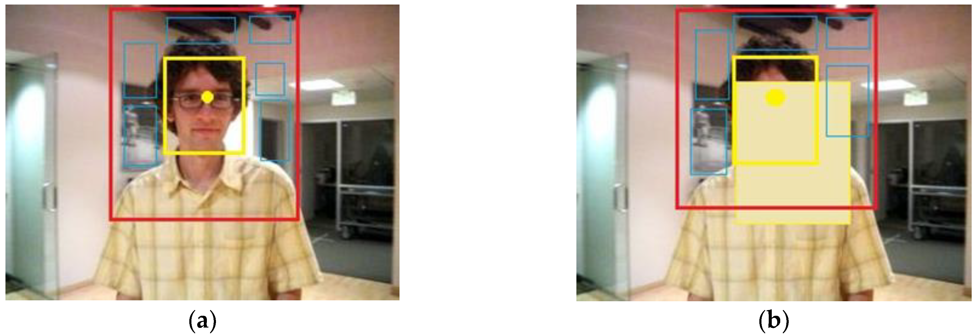
2.1.1. Spatial Context Model

The conditional probability function P ( x , c ( z ) | o ) in Equation (1) is defined as:
P ( x , c ( z ) | o ) = h s c ( x z )
where h s c ( x z ) is a function with respect to the relative distance and direction between the target location x and its local context location z , thereby encoding the spatial relationship between the target and its spatial context [26].

2.1.2. Context Prior Model

In Equation (1), the context prior probability is simply modeled by the following formulation:
P ( c ( z ) | o ) = I ( z ) ω σ ( z x * )
where I ( z ) is the grayscale features of point z in the local context of the target, and ω   is a weighted function defined by:
ω σ ( z ) = a e | z | 2 σ 2
where the smaller the distance from z to   x , the greater the ω   value. The parameter σ is the variance of the Gaussian weight function, which determines the distance threshold. The larger the value of σ is, the wider the field of view will be.

2.1.3. Confidence Map

The confidence map of the target location is modeled as:
c ( x ) = P ( x | o ) = b e | x x * α | β
where b is a normalization constant, α is a scale parameter, and β is a shape parameter. After verification by experiments, the optimal tracking effect is shown when β   = 1.

2.1.4. Fast Learning Spatial Context Model

Our objective is to learn the spatial context model in Equation (2) based on the context prior model in Equation (3) and the confidence map shown in Function (5). Putting Equations (2), (3), and (5) together, Equation (1) becomes:
c ( x ) = b e | x x * α | β = z Ω c ( x * ) h s c ( x z ) I ( z ) ω σ ( z x * ) = h s c ( x ) ( I ( x ) ω σ ( x x * ) )
where c ( x ) is only related to the relative distance of the target neighborhood point x to the target position x * , and denotes the convolution operator.
Equation (6) can be transformed to the frequency domain so that the fast Fourier transform (FFT) algorithm can be utilized for fast convolution as the following formulation.
F ( b e | x x * α | β ) = F ( h s c ( x ) F ( I ( x ) ω σ ( x x * ) ) )
where F denotes the FFT function and is the element-wise product.
As long as the size of the neighborhood box is determined, the confidence graph is a constant matrix that is converted to the frequency domain for calculation and obtaining the spatial context model   h s c ( x ) [26]. The inverse Fourier transform are performed on Equation (7) to get the spatial context model.
h s c ( x ) = F 1 ( F ( b e | x x * α | β ) F ( I ( x ) ω σ ( x x * ) ) )
where F 1 denotes the inverse FFT function.
We exploit the spatial context model to update the spatio-temporal context model as follows:
H t + 1 s t c = ( 1 ρ ) H t s t c + ρ h t s c
where ρ is the learning parameter and h t s c   is the spatial context model computed by Equation (8) at the the t -th frame. Function (9) is the temporal filtering procedure, which can be easily observed in the frequency domain:
H ω s t c = F ω h ω s c
where H ω s t c H t s t c e j ω d t is the temporal Fourier transform of H t s t c and similar to h ω s c . The temporal filter F ω is set as:
F ω = ρ e j ω ( 1 ρ )
where j denotes the imaginary unit. It is easy to validate that F ω in Equation (11) is a low-pass filter [27,28].

2.1.5. Target Tracking

When the ( t + 1 ) -th frame arrives, we crop out the local context region Ω c ( x t * ) based on the tracked location x t * at the t -th frame and construct the corresponding context feature set X t + 1 c = { c ( z ) = ( I t + 1 ( z ) , z ) | z Ω c ( x * ) } .
The object location x t + 1 * in the ( t + 1 ) -th frame is determined by maximizing the new confidence map:
x t + 1 * = argmax x Ω c ( x t * ) c t + 1 ( x )
where c t + 1 ( x ) is represented as:
c t + 1 ( x ) = F 1 ( F ( H t + 1 s t c ( x ) ) F ( I t + 1 ( x ) ω σ t ( x x * ) ) )

2.1.6. The Scale and Variance are Updated as

{ s t = c t ( x t * ) c t 1 ( x t 1 * ) s ¯ t = 1 n i = 1 n s t i s t + 1 = ( 1 λ ) s t + λ s ¯ t σ t + 1 = s t σ t
where c t ( · ) is the confidence map that is computed by Equation (6), and s t is the estimated scale between two consecutive frames. Aiming to avoid oversensitive adaptation and to reduce the noise introduced by the estimation error, the estimated target scale s t + 1 is obtained through filtering in which s ¯ t is the average of the estimated scales from n consecutive frames, and λ > 0 is a fixed filter parameter.

2.2. The Basic Principle of Kalman Filtering Algorithm

The Kalman filter assumes that the system noise and the observed noise are white noise [27]. The system state equation of the discrete dynamic equations for the non-linear systems is defined as:
X k = f ( X k 1 ) + W k 1
The measurement equation is set as:
  Z k = h ( X k ) + V k
where X k R n × 1 is the target state vector. Z k R m × 1 is the observation vector of dimension m. W k R p × 1 is the state noise, V k R m × 1 is the observation noise. W k and V k are the independent Gaussian self-noise vector sequences that are not related to each other.
h ( X k ) = [ r k θ k ] = [ x 2 ( k ) + y 2 ( k ) arctan ( y ( k ) x ( k ) ) ]
where h ( X k ) is the measured equation. The next state prediction is updated by Equation (18):
X ^ k | k 1 = F k | k 1 X ^ k 1 | k 1
and the prediction variance matrix is denoted as:
P k | k 1 = F k | k 1 P k 1 | k 1 F T k | k 1 + Q k 1
where F k | k 1 is the state transition matrix, as shown in Equation (29), X ^ k | k 1 is the predicted state estimator, P k | k 1 is the prediction estimation covariance, and Q k is the covariance matrix.
The dynamic noise variance matrix Q k is expressed by:
Q k = [ 1 0 0 0 0 1 0 0 0 0 1 0 0 0 0 1 ]
The filter gain matrix is signified as:
K k = P k | k 1 H k T [ H k P k | k 1 H k T + R k ] 1
where R k is the measurement of the noise variance matrix.
R k = [ 1 0 0 1 ]
where K k is the optimal Kalman gain. The state estimator is represented as:
X ^ k | k = X ^ k | k 1 + K k Z k Z ^ k | k 1
Z ^ k | k 1 = h ( X ^ k | k 1 )
which is deduced from Equation (18). The estimated error variance matrix is formulated as:
P k | k = [ I K k H k ] P k | k 1
where X ^ k | k is the current updated state estimate, and P k | k is the updated covariance estimate.

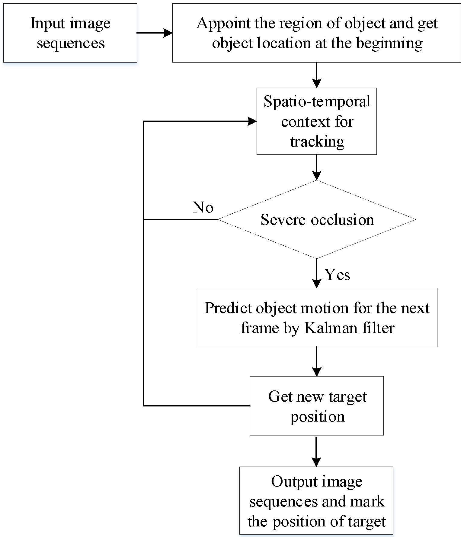
3. STC-KF Target Tracking Algorithm

In the target tracking, the rectangular regions of the tracking object are manually marked in the initial frame, and the confidence map of the frame target is calculated by the spatio-temporal context algorithm. The spatio-temporal context algorithm, as a fast method, mainly adopts fast Fourier transform to calculate each local context region. However, its drawback is that it can easily cause the drift problem. Depending on the advantages and disadvantages of the spatio-temporal context and the Kalman filter algorithm, an improved algorithm combines these two algorithms, which is denoted as STC-KF. Using Fourier transform and inverse transform, we find out the probability of the spatial context condition of the target in the next frame. Then, tracking is conducted in the next frame by calculating the confidence map as a convolution problem, which incorporates the spatio-temporal context information, and the best target location can be estimated by maximizing the confidence map or by the prediction value of the Kalman filter. Specifically, the Kalman filter utilizes the state transition matrix to determine the predicted value of the status with the achieved system status of the ( k 1 ) - th frame, and the state transition matrix is also relevant to the state estimation at the k - th frame. The prediction value of the Kalman filter can be updated as the Kalman observation of the object position and marked on the next frame. Figure 3 is the algorithm flowchart of the STC-KF algorithm.
Based on the estimation function in Equation (25) and the spatio context prior model in Equation (9), our objective is to improve the tracker. It can be formulated as:
H t + 1 s t c k = ( 1 ρ ) H t s t c k + ρ h t s c ( x ) + P k | k
The Gaussian function is introduced into the context prior model in Equation (3) as:
P ( c ( z ) | o ) = I ( z ) 1 2 π σ 2 e | z | 2 σ 2
where I ( z ) is the image intensity of the z point. The parameter σ is the variance of the Gaussian weight function, which determines the distance threshold.
Therefore, our spatio-temporal context model can theoretically effectively filter out the image noise introduced by the appearance variations, thereby leading to more stable results.
When the target is severely obstructed, the Euclidean distance between the grayscale of the t -th frame and the ( t + 1 ) -th frame can be calculated by Equation (28), and the result can be measured as a judgment of whether the target is occluded:
d E ( I t ( z ) , I t 1 ( z ) ) = r t r ( I t ( z i ) I t 1 ( z i ) ) 2
When d E is greater than 17% of the target area and the target center is unchanged but the target is occluded, the program begins with Kalman filter prediction [28].
The Jacobian matrix is shown as:
F k | k = [ 1 0 Δ t 0 0 1 0 Δ t 0 0 1 1 0 0 0 0 ]
The measurement equation is updated as:
m k = [ r k θ k ] = [ ( s x ) 2 + ( s y ) 2 arctan ( ( s y / s x ) ]
where r k is the scope of the observation and θ k is the observation angle. According to Equation (29), the Jacobian matrix that measures the updated equation is:
H k = ( m k ) X k | X k = [ cos ( θ k ) sin ( θ k ) 0 0 sin ( θ k ) / r k cos ( θ k ) / r k 0 0 ]
After updating the error variance matrix in Equations (25) through (31), we can locate the position of the target in each frame by Equation (26), which efficiently reduces the risk of missing the target and improves the stability for tracking.

4. Experimental Results and Analysis

We evaluate the proposed STC-KF tracking algorithm using three representative benchmarks of OTB50/100. In the entire tracking experiment, the platform used a Windows 7 operating system, 3G memory, and 2.20 GHz computer, and was simulated on Matlab2014a platform.

4.1. Database Introduction

OTB50, also named as OTB2013 [29], is a performance evaluation database supplied by CVPR2013. The database OTB 100, also known as database OTB2015 [30], is given in CVPR2015. OTB50 (2013) and OTB100 (2015) respectively include a large dataset with ground-truth object positions and extents for tracking experiments. Specifically, OTB100 contains the video sequences of OTB50, but these two databases are considered as two different video sequences due to different labeling objects. The full benchmark contains 100 sequences from the recent literature. The video set used in this experiment includes three scenes: scene Car with occlusion, scene David with illumination changes, and scene Motocross with pose and contour variation. Among these three scenes, there are 450 frames in Car with the resolution of 290 × 217, 770 frames in David with the resolution of 320 × 240, and 190 frames in Motocross with the resolution of 470 × 310.

4.2. Experimental Results

4.2.1. Scene with Occlusion Condition

In the experiment based on the Car dataset, the position of the initial frame of the target is marked as (140,90,55,31).
As shown in Figure 4, before the 90th frame, the car can be tracked normally, and the STC algorithm can correctly track the target without blocking or drifting. However, when tracking to frame 91 and frame 92, due to the fast-moving speed of the target, the tracking target frame started to shift to the incorrect position. Correspondingly, from frame 97 to frame 105, the target frame continuously missed the correct target. At frame 105, the target box completely missed the target and the target remained in the lost state.
Figure 5 depicts the tracking effect of the STC-KF algorithm on the Car dataset, where the yellow rectangle and red rectangle indicate the target location obtained by the STC-KF algorithm of the STC algorithm and the Kalman filter, respectively. In frame 91 and frame 92, when the background of the car changed drastically, the STC-KF algorithm could normally track the target, which was better than the original STC algorithm. Besides, from frame 165 to 169, the STC-KF algorithm can correctly predict the target when the object was occluded, which solved the target occlusion problem. From frame 358 to frame 365, although the target was in the low light intensity background, the algorithm in this paper still depicted a robust tracking effect.

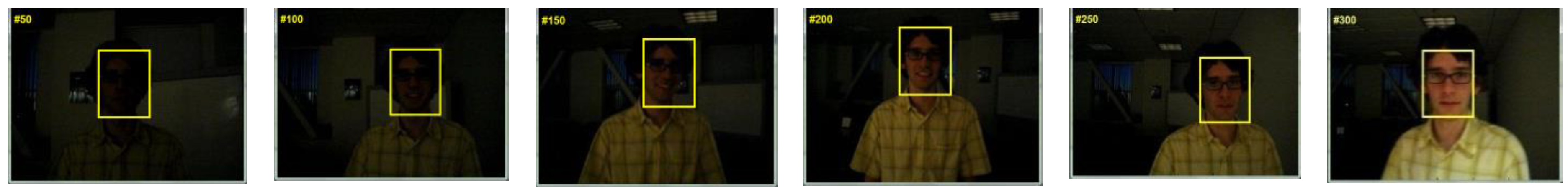
4.2.2. Scene with Illumination Changes Condition

In the experiment based on the David dataset, the position of the initial frame of the target is marked as (161,65,75,95).
It can be seen from the comparison between Figure 6 and Figure 7 that in the 50th frame, both algorithms can track the target in the case of low illumination intensity, but the STC algorithm contains too many redundant regions. Thus, at 100 frames, tracking the face frame was slightly offset; at frame 150, the target can be tracked correctly, but the tracking frame was slightly offset. The STC-KF algorithm was more accurate in tracking the face area of the target, and fewer redundant areas, which indicated that the STC-KF algorithm is superior.

4.2.3. Scene with Pose and Contour Variation Condition

In the experiment based on the Motocross dataset, the position of the initial frame of the target is marked as (288,313,36,78).
Figure 8 depicts the simulation of the Motocross by the STC algorithm. The STC algorithm cannot track the target correctly due to the target vertical gap between two adjacent frames being too large. Figure 9 reveals the simulation of the motocross by the STC-KF algorithm. Indeed, the tracking effect was slightly better than the STC algorithm, but there were occasions when the tracking target was occasionally lost by these two consecutive frames, which have great variation in pose and contour. However, in the vertical direction, the STC-KF algorithm can determine the target position more effectively than the STC algorithm.

5. Performance Analysis

Table 1 shows the correct number of target tracking frames for the STC algorithm and the STC-KF algorithm in the Car experiment. From the table, we can see that in terms of the number of correct tracks frames, the accuracy of the STC-KF algorithm (88.3%) is significantly higher than the accuracy of the STC algorithm (22.2%). Obviously, the proposed algorithm achieves the better performance in terms of success rate.
We can analyze the advantages of our algorithm from the position of the center point.
Table 2 shows the location information of the David video of each target by the STC algorithm and the STC-KF algorithm. According to Table 2, the average error of the STC algorithm is 5.87 pixels, and the average error of the STC-KF algorithm is 2.83 pixels. This shows that the algorithm of this paper is more effective and accurate than the original STC algorithm in target tracking.
In view of the shortcomings of the STC algorithm in the tracking process, this paper combines the STC and the Kalman filter to form the STC-KF algorithm; this algorithm mainly solves the problems of pose and contour variations and the target occlusion. We compare the proposed algorithm of this paper with the original STC algorithm, and the experiments on challenging video sequences show that the proposed STC-KF algorithm achieves favorable performance in terms of accuracy, robustness, and speed.

6. Conclusions

In this paper, we presented a fast and robust algorithm that combines the STC and the Kalman filter to form the STC-KF algorithm. The algorithm mainly solved the problems related to heavy occlusion, illumination changes, and pose and contour variation. By tracking experiments, compared with the STC algorithm, the STC-KF algorithm is robust to severe occlusion, self-position change, and illumination intensity change under the premise of ensuring tracking accuracy. Consequently, the target tracking performance of the proposed algorithm under occlusion condition is superior to that of the STC algorithm.
However, in view of the inaccuracy of tracking in the experiment, there is still room to advance in the tracking effect of strenuous moving targets in serious pose and contour variation condition. In recent years, some sophisticated algorithms have adopted detection algorithms [12,31] or deep learning algorithms [32,33,34], and future work can focus on those algorithms to further improve robustness and tracking accuracy.

Author Contributions

Conceptualization, Z.Z. and D.O.W.; methodology, Z.Z.; software, H.Y.; validation, J.W., Y.M., Y.Y.; investigation, Z.W. and Q.S.; data curation, H.Y., J.W., Y.M., Y.Y.; writing—original draft preparation, H.Y.; writing—review and editing, Z.Z. and Q.S.

Funding

This research was funded by the National Natural Science Foundation of China, grant number 61403281; the Natural Science Foundation of Shandong Province, grant number ZR2014FM002; China Postdoctoral Science Special Foundation Funded Project, grant number 2015T80717; Youth Teachers’ Growth Plan of Shandong Province, grant number 201701.

Acknowledgments

Many thanks for the reviewer and the editors for the insightful comments and suggestions.

Conflicts of Interest

The authors declare no conflict of interest.

References

  1. Kim, M.; Kim, S. Robust appearance feature learning using pixel-wise discrimination for visual tracking. ETRI J. 2019, 41, 483–493. [Google Scholar] [CrossRef]
  2. Zimmermann, K.; Matas, J.; Svoboda, T. Tracking by an optimal sequence of linear predictors. IEEE Trans. Pattern Anal. Mach. Intell. 2009, 31, 677–692. [Google Scholar] [CrossRef] [PubMed]
  3. Ellis, L.; Dowson, N.; Matas, J. Linear regression and adaptive appearance models for fast simultaneous modeling and tracking. Int. J. Comput. Vis. 2011, 95, 154–179. [Google Scholar] [CrossRef]
  4. Kalal, Z.; Mikolajczyk, K.; Matas, J. Forward Backward Error: Automatic Detection of Tracking Failures. In Proceedings of the 20th International Conference on Pattern Recognition (ICPR), Istanbul, Turkey, 23–26 August 2010; pp. 2756–2759. [Google Scholar]
  5. Zhao, Z.S.; Zhang, L.; Zhao, M.; Hou, Z.G.; Zhang, C.S. Gabor face recognition by multi-channel classifier fusion of supervised kernel manifold learning. Neurocomputing 2012, 97, 398–404. [Google Scholar] [CrossRef]
  6. Tzimiropoulos, G.; Zafeiriou, S.; Pantic, M. Sparse representations of image gradient orientations for visual recognition and tracking. In Proceedings of the IEEE Computer Society Conference on Computer Vision and Pattern Recognition Workshops (CVPRW), Colorado Springs, CO, USA, 20–25 June 2011; pp. 26–33. [Google Scholar]
  7. Liwicki, S.; Zafeiriou, S.; Tzimiropoulos, G. Efficient online subspace learning with an indefinite kernel for visual tracking and recognition. IEEE Trans. Neural Netw. Learn. Syst. 2012, 23, 1624–1636. [Google Scholar] [CrossRef]
  8. Mei, X.; Ling, H.B. Robust visual tracking and vehicle classification via sparse representation. IEEE Trans. Pattern Anal. Mach. Intell. 2011, 33, 2259–2272. [Google Scholar]
  9. Wang, Z.X.; Teng, S.H.; Liu, G.D.; Zhao, Z.S. Hierarchical sparse representation with deep dictionary for multi-modal classification. Neurocomputing 2017, 253, 65–69. [Google Scholar] [CrossRef]
  10. Horbert, E.; Rematas, K.; Leibe, B. Level-set person segmentation and tracking with multi-region appearance models and top-down shape information. In Proceedings of the IEEE International Conference on Computer Vision (ICCV), Barcelona, Spain, 6–13 November 2011; pp. 1871–1878. [Google Scholar]
  11. Nicolas, P.; Aurelie, B. Tracking with occlusions via graph cuts. IEEE Trans. Pattern Anal. Mach. Intell. 2011, 33, 144–157. [Google Scholar]
  12. Kalal, Z.; Mikolajczyk, K.; Matas, J. Tracking-Learning-Detection. IEEE Trans. Pattern Anal. Mach. Intell. 2012, 34, 1409–1422. [Google Scholar] [CrossRef]
  13. Pouya, B.; Seyed, A.C.; Musa, B.M.M. Upper body tracking using KLT and Kalman filter. Procedia Comput. Sci. 2012, 13, 185–191. [Google Scholar]
  14. Wang, Y.; Liu, G. Head pose estimation based on head tracking and the Kalman filter. Phys. Procedia 2011, 22, 420–427. [Google Scholar]
  15. Fu, Z.X.; Han, Y. Centroid weighted Kalman filter for visual object tracking. Measurement 2012, 45, 650–655. [Google Scholar] [CrossRef]
  16. Wu, H.; Han, T.; Zhang, J. Target Tracking Algorithm Based on Kalman Filter and Optimization MeanShift. In LIDAR Imaging Detection and Target Recognition; Society of Photo-Optical Instrumentation Engineers (SPIE): Washington, DC, USA, 2017; p. 1060526. [Google Scholar]
  17. Gordon, N.J.; Salmond, D.J.; Smith, A.F.M. Novel Approach to Nonlinear/Non-Gaussian Bayesian State Estimation. IEE Proc. F Radar Signal Process. 1993, 140, 107–113. [Google Scholar] [CrossRef]
  18. Su, Y.Y.; Zhao, Q.J.; Zhao, L.J. Abrupt motion tracking using a visual saliency embedded particle filter. Pattern Recognit. 2014, 47, 1826–1834. [Google Scholar] [CrossRef]
  19. Liu, D.; Zhao, Y.; Xu, B. Tracking Algorithms Aided by the Pose of Target. IEEE Access. 2019, 7, 9627–9633. [Google Scholar] [CrossRef]
  20. Yang, J.P.; Liang, W.T.; Wang, J. A method of high maneuvering target dynamic tracking. In Proceedings of the International Conference on Energy, Environment and Materials Science, Guangzhou, China, 25–26 August 2015; pp. 25–26. [Google Scholar]
  21. Hu, J.; Fang, W.; Ding, W. Visual Tracking by Sequential Cellular Quantum-Behaved Particle Swarm Optimization, Bio-Inspired Computing—Theories and Applications (BIC-TA 2016). In International Conference on Bio-Inspired Computing: Theories and Applications; Springer: Singapore, 2016; pp. 86–94. [Google Scholar]
  22. Sengupta, S.; Peters, R.A. Learning to Track On-The-Fly Using a Particle Filter with Annealed-Weighted QPSO Modeled after a Singular Dirac Delta Potential. In Proceedings of the IEEE Symposium Series on Computational Intelligence (SSCI), Bangalore, India, 18–21 November 2018; pp. 1321–1330. [Google Scholar]
  23. Zhang, K.H.; Zhang, L.; Liu, Q.S. Fast Visual Tracking via Dense Spatio-Temporal Context Learning. In European Conference on Computer Vision; Springer: Cham, Switzerland, 2014; pp. 127–141. [Google Scholar]
  24. Thang, B.D.; Nam, V.; Gerard, M. Context tracker: Exploring supporters and distracters in unconstrained environments. In Proceedings of the IEEE Conference on Computer Vision and Pattern Recognition (CVPR), Colorado Springs, CO, USA, 20–25 June 2011; pp. 1177–1184. [Google Scholar]
  25. Yang, M.; Wu, Y.; Hua, G. Context-aware visual tracking. IEEE Trans. Pattern Anal. Mach. Intell. 2009, 31, 1195–1209. [Google Scholar] [CrossRef]
  26. Wang, H.; Liu, P.; Du, Y. Online convolution network tracking via spatio-temporal context. Multimed. Tools Appl. 2019, 78, 257–270. [Google Scholar] [CrossRef]
  27. Kalman, R.E. A New Approach to Linear Filtering and Prediction Problems. Trans. ASME J. Basic Eng. 1960, 82, 35–45. [Google Scholar] [CrossRef] [Green Version]
  28. Lagos-Álvarez, B.; Padilla, L.; Mateu, J.; Ferreira, G. A Kalman filter method for estimation and prediction of space–time data with an autoregressive structure. J. Stat. Plan. Inference 2019, 203, 117–130. [Google Scholar] [CrossRef]
  29. Wu, Y.; Lim, J.; Yang, M.H. Online Object Tracking: A Benchmark. In Proceedings of the Computer Vision and Pattern Recognition (CVPR), Portland, OR, USA, 23–28 June 2013; pp. 2411–2418. [Google Scholar]
  30. Wu, Y.; Lim, J.; Yang, M.H. Object Tracking Benchmark. IEEE Trans. Pattern Anal. Mach. Intell. 2015, 37, 1834–1848. [Google Scholar] [CrossRef]
  31. Li, J.; Wang, J.Z.; Liu, W.X. Moving Target Detection and Tracking Algorithm Based on Context Information. IEEE Access. 2019, 7, 70966–70974. [Google Scholar] [CrossRef]
  32. Lu, X.; Huo, H.; Fang, T. Learning Deconvolutional Network for Object Tracking. IEEE Access. 2018, 6, 18032–18041. [Google Scholar] [CrossRef]
  33. Zhao, Z.S.; Sun, Q.; Yang, H.R. Compression artifacts reduction by improved generative adversarial networks. EURASIP J. Image Video Process. 2019, 62, 1–16. [Google Scholar] [CrossRef]
  34. Hu, X.; Li, J.; Yang, Y. Reliability verification-based convolutional neural networks for object tracking. IET Image Process. 2019, 13, 175–185. [Google Scholar] [CrossRef]
Figure 1. The illustration of the target context. (a) The definition of local context. (b) The context under heavy occlusion.
Mathematics 07 01059 g001
Figure 2. The structure of the spatio-temporal context (STC) algorithm.
Mathematics 07 01059 g002
Figure 3. The implementation process of the spatio-temporal context and Kalman filtering (STC-KF) algorithm.
Mathematics 07 01059 g003
Figure 4. Target tracking results under occlusion condition via the original STC algorithm, where the red rectangle represents the target position.
Mathematics 07 01059 g004
Figure 5. Target tracking results under the occlusion condition via the STC-KF algorithm, where the yellow rectangle and red rectangle indicate the target location obtained by the STC-KF algorithm of the STC and Kalman filter, respectively.
Mathematics 07 01059 g005
Figure 6. Target tracking results under illumination changes condition via the original STC algorithm, where the red rectangle represents the target position.
Mathematics 07 01059 g006
Figure 7. Target tracking results under occlusion condition via the STC-KF algorithm, where the yellow rectangle denotes the target position.
Mathematics 07 01059 g007
Figure 8. Target tracking results under pose and contour variation condition via the original STC algorithm, where the red rectangle represents the target position.
Mathematics 07 01059 g008
Figure 9. Target tracking results under pose and contour variation condition via the STC-KF algorithm, where the yellow rectangle and red rectangle indicate the target location obtained by the STC-KF algorithm of the STC and the Kalman filter, respectively.
Mathematics 07 01059 g009
Table 1. STC and STC-KF auto tracking contrast frames.
Algorithm NameVideo NameNumber of FramesCorrectly Track Frames
STCcar41091
KF-STCcar410362
Table 2. Location information contrast of two algorithms in David.
Number of FramesTarget Real CoordinatesSTC Tracking CoordinatesSTC-KF Tracking CoordinatesSTC Pixel ErrorSTC-KF Pixel Error
50(120,62)(124,63)(121,61)4.11.4
100(164,63)(169,68)(160,60)7.15
150(142,44)(144,46)(143,42)2.82.2
200(128,31)(136,31)(129,29)82.2
250(180,74)(180,70)(182,73)42.1
300(126,60)(120,53)(130,59)9.24.1

