Equilibrium Joining Strategies in the Geo/Geo^K/1 Queueing System

Abstract

We study strategic behavior in the $Geo/Ge{o}^K/1$ queueing system under both fully observable case and fully unobservable case. Furthermore, equilibrium and socially optimal strategies are obtained according to the available information and the linear utility function. We compare the impact of system parameters on the equilibrium strategies and socially optimal strategies. At the same time, we illustrate the effects of parameters on the obtained equilibrium social benefit. Finally, some numerical examples are presented.

1. Introduction

Due to the widespread application of the queueing systems in the fields of computer networks, management in service system and electronic commerce, studying queueing systems from an economical viewpoint becomes an emerging tendency. It is known that, one of the key steps for properly solving this question is to obtain customer’s strategic behavior. The pioneer of studying queueing systems from an economic view was Naor [1], who studied customer’s strategic behavior in the standard Markovian queueing system under an observable queueing model. Assuming that arriving customers are informed about the queue length and make their own decisions, this model could be seen as the observable case. Afterwards, Edelson and Hildebrand [2] considered the unobservable case. Then, some researchers extended the work of Naor, for example, Johansen and Stidham [3], Mendelson and Whang [4], Stidham [5], Yechiali [6] and so on. Chen and Frank [7] improved Naor’s classic model on condition that both the system and customers used the same discount rate to maximize their expected discounted utility. Erlichman and Hassin [8] discussed the queueing system with priority. In this model, the customers with priority are authorized to overtake part of or all of the customers. Yu et al. [9] studied the equilibrium strategies for almost unobservable and fully unobservable Markovian queueing system with balking and delayed repairs. Besides, some games among the customers in various queueing systems have been studied by many researchers. In these systems, many features are included such as priorities, setup time, vacation, breakdowns, retrial and so on. The monographs Hassin [10], Hassin and Haviv [11], Stidham [12] and Wang [13] summarized a large number of basic models and main approaches in the economic analysis of queueing systems.

Because of the extensive applications of discrete time queueing systems in telephone switching systems and telecommunication networks, the corresponding equilibrium strategies have been studied by many scholars. Takagi [14] discussed a discrete-time queueing model with vacation and obtained some excellent results. Ma et al. [15] analyzed the equilibrium behavior in the discrete-time stochastic service systems with multiple vacations. Liu et al. [16] investigated the equilibrium strategies of customers in a $Geo/Geo/1$ queueing system under single vacation policy or multiple vacations policy. Yang et al. [17] considered the strategic behavior in the discrete-time stochastic service systems with multiple working vacations. Yang et al. [18] considered the strategic behavior in the discrete-time stochastic service systems with server breakdowns and repairs.

An amount of work has been done in the batch service queueing systems, due to the extensive use in the visits of a transportation facility at a certain station, communication systems, computer networks and so forth. Hassin and Haviv [11] considered two servers’ queueing systems with batch service. They proposed this model in terms of transportation services. The first is a bus service and the second is a shuttle service. Customers arrive according to a Poisson process. When the number of waiting customers reaches a certain number, this batch of customers leave. They considered the equilibrium strategy and social optimization. Calvert [19] considered strategic behavior with a continuous time Markovian queueing system and an $M/G^{(M)}/\infty$ queueing system. Economou and Manou [20] studied the equilibrium strategies with the queueing system that the service facility serves all customers at once. Meanwhile, Manou et al. [21] researched into the customer’s strategic behavior when the service facility serves a random number of customers. Boudali and Economou [22,23] dealt with the customer’s equilibrium strategic behavior in a queueing system with catastrophes. The difference between these two models is whether the queueing system accepts or does not accept customers during the repair time. Bountali and Economou [24] considered strategic customers in an $M/M^K/1$ queueing system. They did some research for customer equilibrium strategies in two cases, which are the fully unobservable and the fully observable. Then, Bountali and Economou [25] dealt with the partial information about the model above Bountali and Economou [24].

Models with some kinds of batch service with discrete time appear in various situations in practice. For instance, there are bulk signals that need to be served in neural networks. The $Geo/Ge{o}^K/1$ queueing system counts a time slot as a unit, which is more suitable for computer and telecommunication system modeling. In telecommunications, a batch can corresponds to a message while a customer correspond to a packet. At a bus station, each bus serves a stochastical number of customers at a fixed time. This is the same as at an airport, where each plane will take off a batch of customers one time. Therefore, in real life, there are a lot of discrete time batch services.

As far as we know, there are no papers that study strategic behavior in the $Geo/Ge{o}^K/1$ queueing system. This motivates us to explore the economic significance of bulk service queue, because it is more practical under many specific circumstances. In the first place, we extend the research of Bountali and Economou [24] to the $Geo/Ge{o}^K/1$ queueing system. What is more, the $Geo/Ge{o}^K/1$ queueing system is more suitable for analyzing and modeling digital communication. The main objective of this paper is to study the strategic behavior in a $Geo/Ge{o}^K/1$ queueing system. There are fully observable cases and fully unobservable cases to be analyzed. In addition, we use some numerical experiments to reveal the effect of several parameters, as well as information on strategic behavior, and compare it with other stochastic service systems.

This paper is organized as follows. In Section 2, we give the description of the discrete-time batch queueing model and the reward-cost structure. In Section 3, we study the fully observable case and resolve the equilibrium strategy. In this case, we consider the expected total net social benefit per time unit in the discrete-time batch service queueing systems. Subsequently, in Section 4, we study the equilibrium strategies and the socially optimal strategies in the fully unobservable case. In Section 5 we provide several numerical results and illustrate the effect of argument on strategic behavior. Finally, in Section 6, we provide conclusions and give directions for future research.

2. Model Description

We consider a $Geo/Ge{o}^K/1$ queueing system. In this paper, we denote that $\overline{x}=1-x$ for $x\in [0,1]$. The $Geo/Ge{o}^K/1$ queueing system is described as follows:

• Assume that when the number of the customer in the $Geo/Ge{o}^K/1$ queueing system is less than K, the server stops providing service. However, the server provides service when the number of the customers reaches or even exceeds K and serves K customers one time. K is a fixed constant and $K⩾2$.
• Assume that the arrival of potential customer occurs at the end of slot $t=n^{-},n⩾0.$ The inter-arrival times T are independent and identically distributed sequence. Each of them follows geometric distribution with rate p.

  $$P(T=k)=p·{\overline{p}}^{k-1},k=1,2,\cdots ,p\in (0,1).$$
• The beginning and ending of the batch service take place at slot division point $t=n,n⩾0.$ The batch service times $S_n$ are independent of each other and geometrically distributed with rate $\mu$.

  $$\begin{array}{c}\hfill P(S_n=k)=\mu ·{\overline{\mu }}^{k-1},k=1,2,\cdots ,0<\mu <1.\end{array}$$
• We assume that service times and inter-arrival times are mutually independent. The service discipline is taken to be First-Come-First-Served $(FCFS)$. The traffic intensity is given by $\rho =\frac{p}{K\mu }$. Moreover, it is assumed that the system is stable, that is, $\rho <1$.

We focus on researching the strategic behavior of the customers in our model. Upon arrival, the tagged customer has the right to decide whether to join the queue. Suppose that R is the reward to the tagged customer for completing service, C is the cost per time unit spent in the $Geo/Ge{o}^K/1$ queueing system. W is the expected waiting time (included service time). The expected benefit of the tagged customer is

$$B=R-C·W$$

(1)

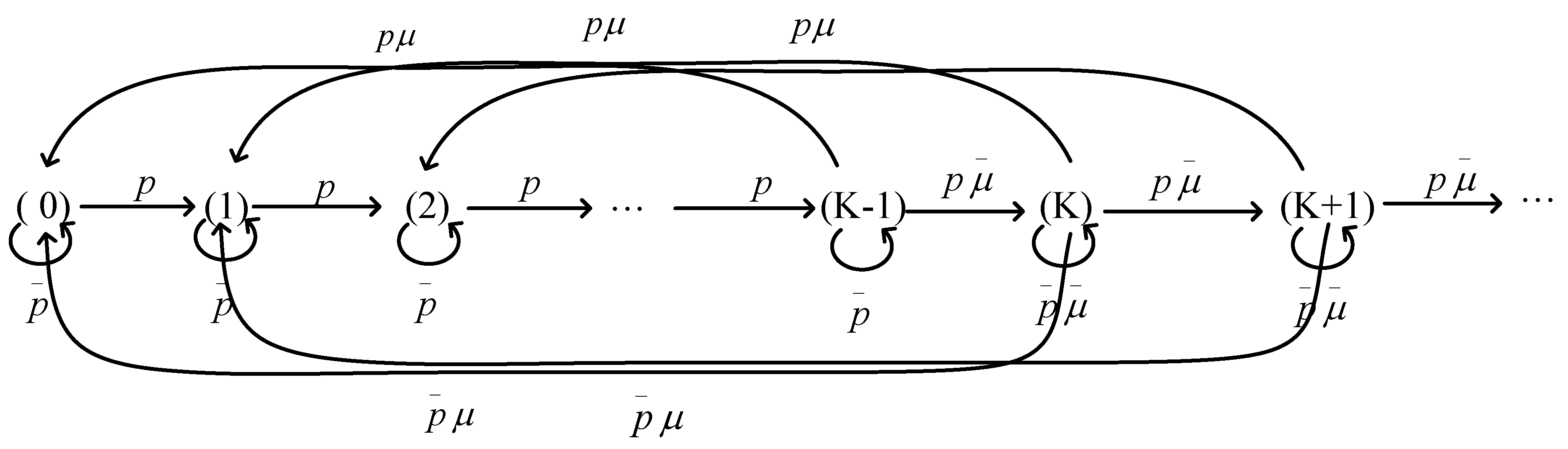
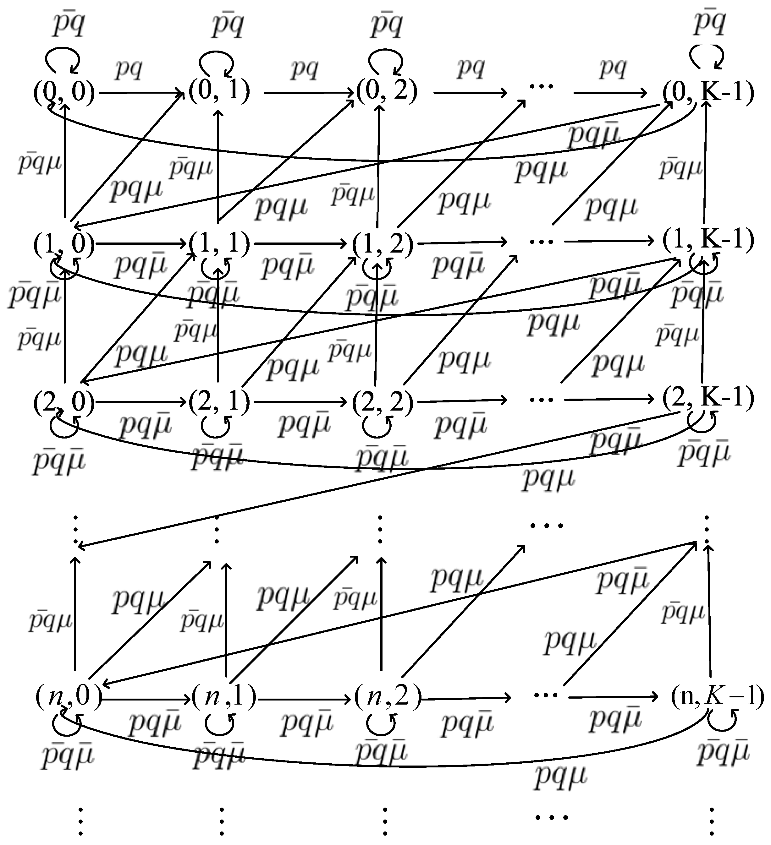
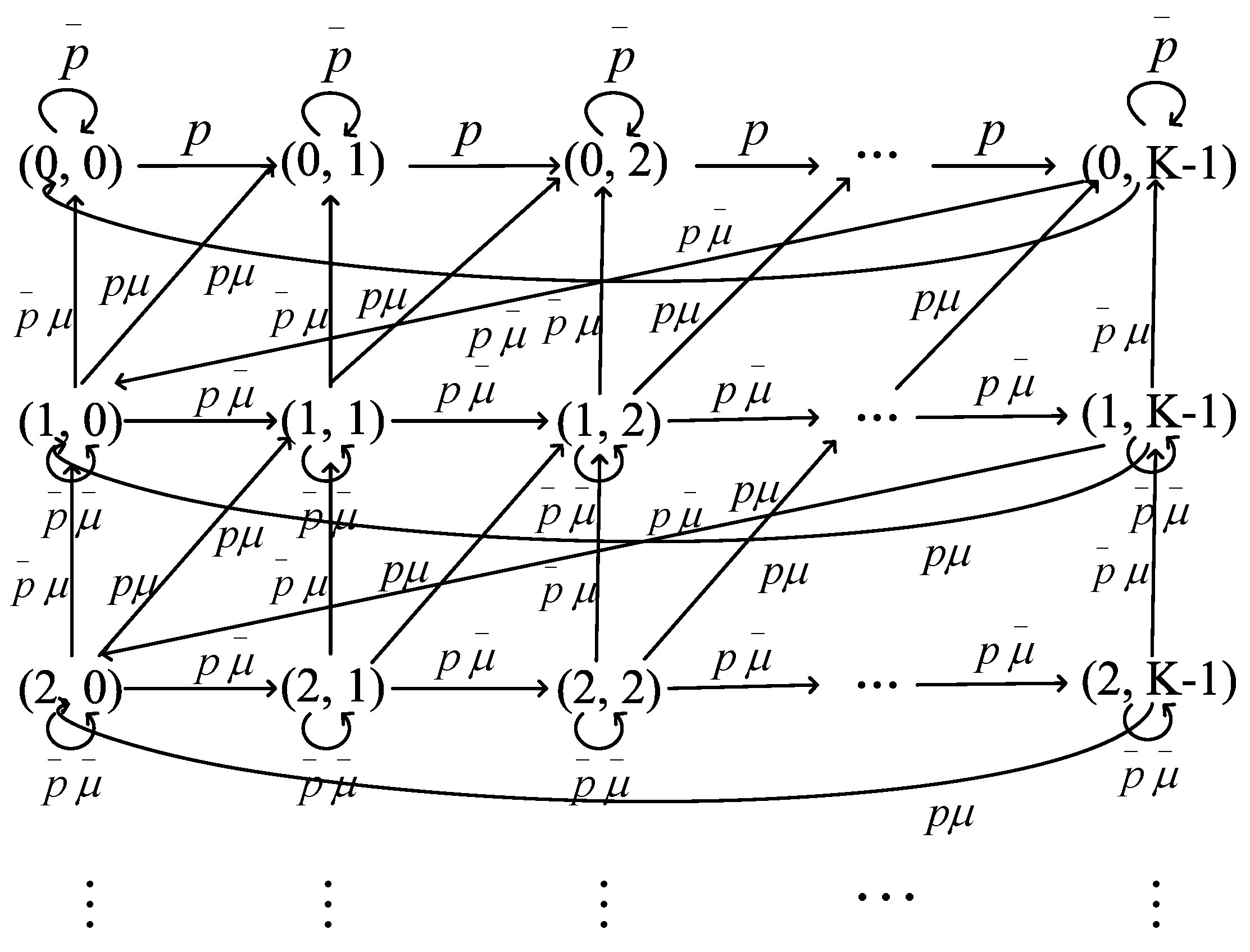
We assume that the number of customers in the queueing system at epoch $n^{+}$ is $L_n$. K is the number of service per batch, which is a constant. We denote that $M_n=[\frac{L_n}{K}]$, where $[x]$ is the largest integer not exceeding x. $J_n=L_n-K·M_n$. It is clear that $L_n$ and $\{(M_n,J_n):n⩾0\}$ are Markov chain. And their state spaces are $\mathsf{\Omega }=\{k|k=0,1,2,\cdots ,\}$ and $\{(m,j)|m=0,1,2,\cdots ;j=0,1,2,\cdots ,K-1\}$, respectively. Their transition rate diagrams are given in Figure 1 and Figure 2.

In this paper, we consider two cases—the fully observable case and the fully unobservable case. Where the fully observable case is that customers observe $(M_n,J_n)$ and the fully unobservable case is customers observe neither $M_n$ nor $J_n$. We assume that customers are risk neutral and maximize their expected net benefit. Finally, we emphasize that the decisions are irrevocable, which means reneging of entering customers and retrials of balking customers are not allowed.

3. The Fully Observable Case

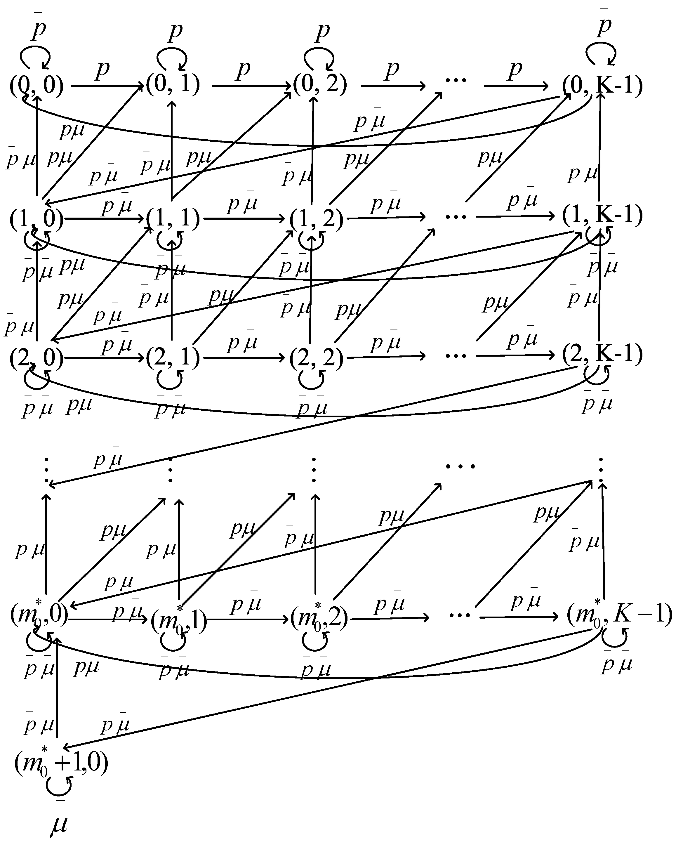
In this section, we study the fully observable case, where the tagged customer has information on the state of the queueing system when they make their decisions, that is, $(M_n,J_n)=(m,j)$. We denote that the equilibrium strategy is $(m_{K-1}^e,q_{(m,j)}^e)$ at the state $(m,j)$. Its state space is ${\mathsf{\Omega }}_{fo}=\{(m,j):0⩽m⩽m_0^{*},0⩽j⩽K-1\}\bigcup \{(m_0^{*}+1,0)\}$ and its transition rate diagram is shown in Figure 3.

The following theorem gives the equilibrium strategy in the fully observable case with the $Geo/Ge{o}^K/1$ queueing system.

Theorem 1.

In the fully observable $Geo/Ge{o}^K/1$ queue, let $(m_{K-1}^e,q_{(m,j)}^e)$ be the equilibrium balking strategy at the state $(m,j)$. There exists a unique equilibrium strategy $q_{(m,j)}^e$ given by

$$q_{(m,j)}^e=\left\{\begin{array}{cc}0,\hfill & ifm>m_j^e,\hfill \\ 1,\hfill & ifm⩽m_j^e,\hfill \end{array}\right.$$

(2)

where

$$m_{K-1}^e=\left[\frac{\mu R}{C}-1\right],$$

$$m_0^e⩽m_1^e⩽\dots ⩽m_{K-1}^e.$$

(3)

Proof. 

We consider the fully observable case in which the tagged customer has information on both m and j. The tagged customer will join the system when he observes state $(m,K-1)$. We can get the expected net benefit:

$$B_{(m,K-1)}^{(o)}=R-\frac{m+1}{\mu }C.$$

The tagged customer prefers to join if and only if $B_{(m,K-1)}^{(o)}$ is non–negative. $q_{(m,K-1)}^e$ is given as follows:

$$q_{(m,K-1)}^e=\left\{\begin{array}{cc}0,\hfill & \mathrm{if}m>m_{K-1}^e,\hfill \\ 1,\hfill & \mathrm{if}m⩽m_{K-1}^e,\hfill \end{array}\right.$$

with $m_{K-1}^e=[\frac{\mu R}{C}-1]$. If $q_{(m,K-1)}^e=0$, then $B_{(m,K-1)}^{(o)}=R-\frac{m+1}{\mu }C<0$.

$$B_{(m,K-2)}^{(o)}=R-\left(\frac{1}{p}+\frac{m+1}{\mu }\right)C<B_{(m,K-1)}^{(o)}<0.$$

We obtain that $q_{(m,K-2)}^e=0$. In fact, we get that the expected net benefit of a customer at state $(m,K-2)$ is less than the expected net benefit of the tagged customer at state $(m,K-1)$. Similarly, we get that $S^{(o)}(m,K-2)$ is increasing in $m\in (0,+\infty )$ and the mean sojourn time in unbounded. Hence, there exists unique $m_{K-2}^e$ such that $\frac{R}{C}\in [S^{(o)}(m_{K-2}^e,K-2),S^{(o)}(m_{K-2}^e+1,K-2))$. The equilibrium strategy $q_{(m,K-2)}^e$, $(m⩾0)$ is given as follows:

$$q_{(m,K-2)}^e=\left\{\begin{array}{cc}0,\hfill & \mathrm{if}m>m_{K-2}^e,\hfill \\ 1,\hfill & \mathrm{if}m⩽m_{K-2}^e.\hfill \end{array}\right.$$

We could conclude that $m_{K-2}^e⩽m_{K-1}^e$ whenever $q_{(m,K-1)}^e=0$.

Similarly, (2) and (3) is still true for $j=K-3,K-4,\cdots ,0.$ Because the decision of the tagged customer at the state when $J_n=j$ depends only the decision of the tagged customer when $J_n>j,$ the equilibrium strategy is unique. □

Next, we need to determine the uniqueness of strategy $(q_{m,j}^e:m=0,1,2,\cdots ,$ $j=0,1,2,\cdots ,K-1)$ by ascertaining the threshold value of $m_j^e,0⩽j⩽K-1$. From Bountali and Economou [24], we obtain that $q_{(m,j)}^e=1$ implies that $q_{(n,i)}^e=1$ when $n⩽m$ and $i⩾j$. However, if we want to calculate the value of strategy $q_{(m,j)}^e:m=0,1,2,\cdots ,j=0,1,2,\cdots ,K-1,$ we must calculate the mean sojourn time of the tagged customer. Theorem 2 gives the calculation formula of the mean sojourn time $S^{(o)}(m,j)$ and the characteristic of thresholds, $m_j^e,0⩽j⩽K-1$.

Theorem 2.

In the fully observable $Geo/Ge{o}^K/1$ queue, suppose $S^{(o)}(m,j)$ is the conditional mean sojourn time, when the tagged customer arrives and observes the system at the state of $(m,j)$, the tagged customer decides to join. Future customers at the system will also join the queue until the tagged customer’s batch completion. Then, $S^{(o)}(m,j)$ can be calculated by the following recurrence

$$S^{(o)}(0,j)=\frac{K-1-j}{p}+\frac{1}{\mu },0⩽j⩽K-1.$$

(4)

$$S^{(o)}(m,K-1)=\frac{m+1}{\mu },m⩾0.$$

(5)

$$\begin{array}{cc}\hfill & S^{(o)}(m,j)=\frac{1}{1-\overline{p}\overline{\mu }}+\frac{p\overline{\mu }}{1-\overline{p}\overline{\mu }}{S}^{(o)}(m,j+1)+\frac{\overline{p}\mu }{1-\overline{p}\overline{\mu }}{S}^{(o)}(m-1,j)\hfill \\ \hfill & +\frac{p\mu }{1-\overline{p}\overline{\mu }}{S}^{(o)}(m-1,j+1),m⩾1and0⩽j⩽K-2.\hfill \end{array}$$

(6)

alternatively

$$\begin{array}{c}\hfill S^{(o)}(m,j)=\frac{m+1}{\mu }+\sum _{i=0}^{K-j-1}\frac{(K-j-1-i)p^{i-1}}{{\overline{p}}^i}\sum _{l=0}^{\infty }\left({}_i^l\right)\left({}_{l-1}^{m-1}\right){\left(\mu \overline{p}\right)}^l{\overline{\mu }}^{m-l},\\ \hfill m⩾0,0⩽j⩽K-1.\end{array}$$

(7)

In addition, $S^{(o)}(m,j)$ has the following properties:

1. 

For any fixed $m⩾0$, $S^{(o)}(m,j)$ is decreasing in $0⩽j⩽K-1$.

2. 

For a fixed j with $j=0,1,2,\cdots ,K-1,S^{(o)}(m,j)$ is increasing in $m\in (0,m_0^{*}+1)$.

3. 

$\underset{m\to \infty }{lim}{S}^{(o)}(m,j)=\infty ,j=0,1,2,\cdots ,K-1$.

For the unique equilibrium strategy $(q_{m,j}^e)$ given by (2), the thresholds $m_j^e,j=0,1,2,\cdots ,K-1$ are obtained by the following recurrence:

$$m_{K-1}^e=\left[\frac{\mu R}{C}-1\right]$$

$$\begin{array}{c}\hfill m_j^e=max\{m:0⩽m⩽m_{j+1}^{e}and{S}^{(o)}(m,j)⩽\frac{R}{C}\},\\ \hfill j=K-2,K-3,\dots ,0.\end{array}$$

(8)

Proof. 

First, we take a tagged customer who finds the server at state $(0,j)$ upon arrival into account. If he decides to enter, he will wait for $K-j-1$ customers to arrive and then complete his own batch (expected waiting time $\frac{K-j-1}{p}$). Next, the tagged customer’s batch will start service (average service time $\frac{1}{\mu }$) and the mean sojourn time of stay in the system is given by (5).

Second, we research a tagged customer who joins the system when the state is $(m,K-1)$. He does not have to wait and directly accepts the service. Therefore $S^{(o)}(m,K-1)$ equals $\frac{m+1}{\mu }$ and we can get (7).

Finally, we deal with a tagged customer who finds the server at state $(m,j)$ and joins, for $m=1,2,\cdots$ and $0⩽j⩽K-2$. Applying the law of total expectation, implies

$$\begin{array}{cc}\hfill S^{(o)}(m,j)=& \overline{p}\overline{\mu }(S^{(o)}(m,j)+1)+\overline{p}\mu (S^{(o)}(m-1,j)+1)\hfill \\ \hfill & +p\overline{\mu }(S^{(o)}(m,j+1)+1)+p\mu (S^{(o)}(m-1,j+1)+1).\hfill \end{array}$$

(9)

p and $\mu$ have the following relationship:

$$\overline{p}\overline{\mu }+\overline{p}\mu +p\overline{\mu }+p\mu =1$$

(10)

Substituting (10) in (9), we obtain (6).

The tagged customer decides to join when the state is $(m_j^{*},j),0⩽j⩽K-1$, his the expected net benefit is

$$B_{(m_j^e,j)}^{(o)}=R-S^{(o)}(m_j^e,j)C⩾0.$$

So we derive the Equation (8). On the other hand, we are interested in getting the expression for the mean sojourn time. In fact, we have that

$$S^{(o)}(m,j)=E[max\{X_m,Y_{K-j-1}\}]+\frac{1}{\mu },m⩾1,0⩽j⩽K-2$$

(11)

where $X_m$ and $Y_{K-j-1}$ are Pascal distribution $(m,\mu )$ and Pascal distribution $(K-j-1,p)$ independent random variable. We denote $N(X_m)$ is the number of new arrival customers during the whole service time $X_m$. Conditioning on $N(X_m)$, we obtain that

$$\begin{array}{cc}\hfill S^{(o)}(m,j)& =E[max\{0,Y_{K-j-1}-X_m\}]+\frac{1}{\mu }+E(X_m)\hfill \\ \hfill & =\frac{m+1}{\mu }+\sum _{i=0}^{\infty }Pr[N(X_m)=i]E[max\{0,Y_{K-j-1}-X_m\}|N(X_m)=i]\hfill \\ \hfill & =\frac{m+1}{\mu }+\sum _{i=0}^{K-j-1}\frac{K-j-1-i}{p}Pr[N(X_m)=i]\hfill \\ \hfill & =\frac{m+1}{\mu }+\sum _{i=0}^{K-j-1}\frac{K-j-1-i}{p}\sum _{l=0}^{\infty }Pr[N(X_m)=i|X_m=l]Pr(X_m=l)\hfill \\ \hfill & =\frac{m+1}{\mu }+\sum _{i=0}^{K-j-1}\frac{(K-j-1-i)p^{i-1}}{{\overline{p}}^i}\sum _{l=0}^{\infty }\left({}_i^l\right)\left({}_{l-1}^{m-1}\right){\left(\mu \overline{p}\right)}^l{\overline{\mu }}^{m-l}.\hfill \end{array}$$

Then, we obtain (7) for $m⩾1$ and $0⩽j⩽K-2$. Similarly (4) and (5) yield (7) for $m=0$ and $j=K-1$. □

In the next subsection, we consider social optimization. According to the above analysis, ${\pi }^{(o)}(m_0^{*}+1,0;m_0^{*})$ is balking probability. When the customer follows the threshold polity $m_0^{*}$ which is given by Theorem 2, we obtain that the expected total net social benefit per time unit as follows:

$$\begin{array}{cc}\hfill & B^{(o)}(m_0^{*})=pR(1-{\pi }^{(o)}(m_0^{*}+1,0;m_0^{*}))\hfill \\ \hfill & -C\sum _{(m,j)\in S_{MJ}^o(m_0^{*})}\left(mK+j\right){\pi }^{(o)}\left(m,j;m_0^{*}\right),\hfill \end{array}$$

where $({\pi }^{(o)}(m,j;m_0^{*}):(m,j)\in S_{MJ}^o(m_0^{*}))$ is the stationary distribution of $\{(M_n,J_n)\}$. However, $({\pi }^{(o)}(m,j;m_0^{*}))$ cannot be solved analytically. Therefore, the optimization and evaluation of $B^{(o)}(m_0^{*})$ can only be carried out numerically.

4. The Fully Unobservable Case

In this part, we consider the fully unobservable queues. The arriving customers do not receive any information about $M_n$ and $J_n$. In the fully unobservable case, the tagged customer’s mixed joining strategies can be described by the probability of $q(0⩽q⩽1)$. The effective arrival rate is $pq$. Figure 4 is the state transition diagram.

Next, we study the mean sojourn time of a tagged customer and the strategic behavior in the $Geo/Ge{o}^K/1$ with an unobservable case.

Theorem 3.

Consider the fully unobservable $Geo/Ge{o}^K/1$ queue, in which the other customers enter with probability q. The equation

$$\mu \overline{pq}{z}^{K+1}+\mu pq{z}^K-(1-\overline{pq}\overline{\mu })z+pq\overline{\mu }=0,pq⩾K\mu ,$$

(12)

has solution $\beta (q)$ in $(0,1)$. The mean sojourn time of a tagged customer is given by:

$$S^{(u)}(q)=\left\{\begin{array}{cc}\infty ,\hfill & ifpq=0orpq⩾K\mu ,\hfill \\ \frac{\beta (q)}{(1-\beta (q))pq}+\frac{K-1}{2pq},\hfill & if0<pq<K\mu ,\hfill \end{array}\right.$$

(13)

Furthermore, the function $S^{(u)}$(q) is strictly convex in the subset of $[0,1]$.

Proof. 

We think over the first case where $q=0$. In this case, no customer enters the system. The tagged customer’s batch will never complete the service. Since $K⩾2$, the mean sojourn time of the arriving customer is infinite. If $q>0$, the queueing system is $Geo/Ge{o}^K/1$ queue with arrival rate $pq$ and service rate $\mu$. This queueing system is stable if and only if $pq<K\mu$. Then, we obtain that $Geo/Ge{o}^K/1$ queue is unstable when $pq⩾K\mu$. We come to the following conclusion $S^{(u)}(q)=\infty$ when $pq⩾K\mu$. So the first branch of (13) is true.

In the second case, for $0<pq<K\mu$ and the stationary analysis in discrete time, the system follows a discrete-time Markov chain ($DTMC$) with state spaces restricted to $\mathsf{\Omega }=\{k|k=0,1,2,\dots \}$. We show the transition rate diagram in Figure 4. We denote L as the number of customers in the system at the steady state. Its distribution is denoted as

$${\pi }_k=P\{L=k\},k\in \mathsf{\Omega }.$$

Based on the one-step transition situation analysis, the one-step transition probability matrix P of the Markov Chain $\{L_n,n=0,1,2,\dots \}$ can be written as:

$$P=\begin{array}{ccccccccc}& 0& 1& 2& \cdots & K-1& K& K+1& \cdots \\ \hfill \left.\begin{array}{c}0\\ 1\\ 2\\ ⋮\\ K-1\\ K\\ K+1\\ ⋮\end{array}\right(& \begin{array}{c}\overline{pq}\\ \\ \\ \\ pq\mu \\ \overline{pq}\mu \\ \\ \cdots \end{array}& \begin{array}{c}pq\\ \overline{pq}\\ \\ \\ \\ pq\mu \\ \overline{pq}\mu \\ \cdots \end{array}& \begin{array}{c}\\ pq\\ \overline{pq}\\ \\ \\ \\ pq\mu \\ \ddots \end{array}& \begin{array}{c}\\ \\ pq\\ \ddots \\ \\ \\ \\ \ddots \end{array}& \begin{array}{c}\\ \\ \\ \ddots \\ \overline{pq}\\ \\ \\ \end{array}& \begin{array}{c}\\ \\ \\ \\ pq\overline{\mu }\\ \overline{pq}\overline{\mu }\\ \\ \end{array}& \begin{array}{c}\\ \\ \\ \\ \\ pq\overline{\mu }\\ \overline{pq}\overline{\mu }\\ \end{array}& \left.\begin{array}{c}\\ \\ \\ \\ \\ \\ pq\overline{\mu }\\ \ddots \end{array}\right)\end{array}$$

Because $\pi P=\pi$, the balanced equations for the stationary distribution are given by:

$${\pi }_0=\overline{pq}{\pi }_0+pq\mu {\pi }_{K-1}+\overline{pq}\mu {\pi }_K,$$

(14)

$${\pi }_i=pq{\pi }_{i-1}+\overline{pq}{\pi }_i+pq\mu {\pi }_{K-1+i}+\overline{pq}\mu {\pi }_{K+i},i=1,2,\dots ,K-1,$$

(15)

$${\pi }_i=pq\overline{\mu }{\pi }_{i-1}+\overline{pq}\overline{\mu }{\pi }_i+pq\mu {\pi }_{K-1+i}+\overline{pq}\mu {\pi }_{K+i},i=K,K+1,\dots .$$

(16)

The probability generating function (PGF) is given by

$$P(z)=\sum _{n=0}^{\infty }{\pi }_n{z}^n.$$

From Equations (14)–(16),we can obtain

$$P(z)=\frac{(1-z^K)\mu [(\overline{pq}+pqz){\sum }_{n=0}^{K-2}{\pi }_n{z}^n+\overline{pq}{\pi }_{K-1}{z}^{K-1}]}{\overline{\mu }pq{z}^{K+1}-(1-\overline{\mu }\overline{pq})z^K+\mu pqz+\mu \overline{pq}}.$$

Therefore, the stationary probability $\{{\pi }_n,n\in N\}$ is given by:

$${\pi }_n=\left\{\begin{array}{cc}\frac{1-\beta {(q)}^{n+1}}{K},\hfill & n=0,1,2,\dots ,K-1;\hfill \\ \frac{\beta {(q)}^{n+1-K}-\beta {(q)}^{n+1}}{K},\hfill & n=K,K+1,\dots .\hfill \end{array}\right.$$

(17)

We obtain:

$$E[L]=\sum _{n=0}^{\infty }n{\pi }_n=\frac{d}{dz}\left[P(z)\right]{|}_{z=1}=\frac{K-1}{2}+\frac{\beta (q)}{1-\beta (q)}.$$

(18)

Using Equation (18) and Little’s law, we can obtain the second branch of (13).

As we all know that the function of the coefficients $C^{\infty }$ determines the single root of the polynomial (see Lozada [26]). For $z=\beta (q)$, the derivation of (12) and the second-order derivative with respect to q are

$${\beta }^{\prime }(q)=\frac{p(1-\beta (q))(\mu \beta {(q)}^K+\overline{\mu })}{1-\overline{pq}\overline{\mu }-K\mu pq\beta {(q)}^{K-1}-(K+1)\mu \overline{pq}\beta {(q)}^K},$$

(19)

$${\beta }^{″}(q)=\frac{D+E}{1-\overline{pq}\overline{\mu }-K\mu pq\beta {(q)}^{K-1}-(K+1)\mu \overline{pq}\beta {(q)}^K},$$

(20)

respectively. Where

$$D={\beta }^{\prime }(q)[-2(K+1)\mu p\beta {(q)}^K+(K+1)K\mu \overline{pq}\beta {(q)}^{K-1}{\beta }^{\prime }(q)],$$

$$E={\beta }^{\prime }(q)[K(K-1)\mu pq\beta {(q)}^{K-2}{\beta }^{\prime }(q)+2K\mu p\beta {(q)}^{K-1}-2p\overline{\mu }].$$

The second order derivative of $S^{(u)}(q)$ given in the second branch of (13) is

$${S^{(u)}}^{″}(q)=G+H,$$

(21)

where

$$G=\frac{(K-1)}{p{q}^3}+\frac{2\beta (q)}{p{q}^3(1-\beta (q))}-\frac{2{\beta }^{\prime }(q)}{pq{(1-\beta (q))}^2},$$

$$H=\frac{2{\beta }^{\prime }{(q)}^2}{pq{(1-\beta (q))}^3}+\frac{{\beta }^{″}(q)}{pq{(1-\beta (q))}^2}.$$

Using the chain rule and taking into account (19) and (20), we can obtain that: $S^{{(u)}^{″}}(q)>0$. The strict convexity of $S^{(u)}(q)$ is shown. □

Next, we study the equilibrium joining strategies of the tagged customer in the fully unobservable case. Theorem 4 indicates the characteristic and the quantities of the equilibrium joining strategy.

Theorem 4.

Consider the fully unobservable model of the $Geo/Ge{o}^K/1$ queue, suppose $q_{min}$ is the unique point that globally minimizes the second branch of $S^{(u)}(q)$ in (13). The equilibrium strategies followed by each tagged customer are:

Case 

I: $S^{(u)}(q_{min})<\frac{R}{C}$. Because of the strict convexity of $S^{(u)}(q)$, the equation $S^{(u)}(q)=\frac{R}{C}$ have two roots $q_1$ and $q_2$. Let $q_1<q_2$,

–

Ia: If $q_1>1$, there is a unique equilibrium strategy: $q^e=0$.

–

Ib: If $q_1=1$, there are two equilibrium strategies: $q^e=0$ and $q^e=1$.

–

Ic: If $q_1<q_2<1$, there are three equilibrium strategies: $q^e=0,q^e=q_1$ and $q^e=q_2$.

–

Id: If $q_1<1<q_2$, there are three equilibrium strategies: $q^e=0,q^e=q_1$ and $q^e=1$.

Case 

II: $S^{(u)}(q_{min})=\frac{R}{C}$.

–

IIa: If $q_{min}⩽1$, there are two equilibrium strategies: $q^e=0$ and $q^e=q_{min}$.

–

IIb: If $q_{min}>1$, there is a unique equilibrium strategy: $q^e=0$.

Case 

III: If $S^{(u)}(q_{min})>\frac{R}{C}$, there is a unique equilibrium strategy: $q^e=0$.

Proof. 

First, we consider the case when $q=0$. In this case, the expected value of the sojourn time of a tagged customer is infinite. The strategy $q=0$ of balking is always an equilibrium strategy.

When $S^{(u)}(q_{min})<\frac{R}{C}$, there are two roots of the equation $S^{(u)}(q)=\frac{R}{C}$. The roots of the equation are $q_1$ and $q_2$ ($q_1<q_2$). When $q_1>1$, there exists a unique equilibrium strategy $q^e$: $q^e=0$ (subcase Ia). When $q_1=1$, there exist two equilibrium strategies $q^e$: $q^e=0$ and $q^e=1$ (subcase Ib). In the subcase Ic, if $q_1<q_2<1$, then $q_1$ and $q_2$ are the equilibrium strategies. Therefore, there are three equilibrium strategies: $q^e=0$, $q^e=q_1$ and $q^e=q_2$ (subcase Ic). If $q_1<1<q_2$, then $q_2$ is not the equilibrium strategy. In the case, the equilibrium strategies are $q^e=q_1,q^e=1$ and $q^e=0$ (subcase Id).

Next, in the case II, when $q_{min}>1$, the equation $S^{(u)}(q)=\frac{R}{C}$ has no solution in $(0,1)$. So there is a unique equilibrium strategy $q^e=0$ (subcase IIb). When $q_{min}⩽1$, the equation $\frac{R}{C}=S^{(u)}(q)$ has a solution: $q_{min}$, so there are two equilibrium strategies $q^e=0$ and $q^e=q_{min}$ (subcase IIa).

Finally, in the case III, $S^{(u)}(q_{min})>\frac{R}{C}$, the tagged customer prefer to balk, so there is a equilibrium strategy $q^e=0$. □

According to Theorem 4 and Bountali and Economou [24], we are surprised to find that the strategy 0 is always an equilibrium strategy, both a continuous time batch service queueing system and a discrete time batch service queueing system. The result is a significant difference between the model with single service $(K=1)$ and the model with authentic batch services $(K⩾2)$.

We now consider the problem of the expected total net social benefit per time unit maximization $B^{(u)}(q)$ with respect to strategy q, which should be imposed on the customers. According to (13), we can obtain

$$\begin{array}{cc}\hfill B^{(u)}(q)& =pq(R-C{S}^{(u)}(q))\hfill \\ \hfill & =\left\{\begin{array}{cc}-\infty ,\hfill & \mathrm{if}pq⩾K\mu ,\hfill \\ 0,\hfill & \mathrm{if}pq=0,\hfill \\ pqR-C\left({\displaystyle \frac{\beta (q)}{1-\beta (q)}}+{\displaystyle \frac{K-1}{2}}\right),\hfill & \mathrm{if}0<pq<K\mu .\hfill \end{array}\right.\hfill \end{array}$$

(22)

We can show that the non-constant third branch of $B^{(u)}(q)$ is unimodal respect to p. We can now study the socially optimal strategies.

Theorem 5.

In the fully unobservable $Geo/Ge{o}^K/1$ queue, the quantities and the type of the socially optimal strategies depend on the values of $q_{max}$ and $q_{min}$, where $q_{max}$ is the unique point that globally maximizes the third branch of (22), and $q_{min}$ is the unique point that globally minimizes the second branch of (13).

Case 

I: If $S^{(u)}(q_{min})<\frac{R}{C}$, then there exists a unique socially optimal strategy: $q^{soc}=min(q_{max},1)$.

Case 

II: $S^{(u)}(q_{min})=\frac{R}{C}$.

–

IIa: If $q_{min}>1$, then there exists a unique socially optimal strategy: $q^{soc}=0$.

–

IIb: If $q_{min}⩽1$, then there exist two socially optimal strategies: $q^{soc}=0$ and $q^{soc}=q_{min}$.

Case 

III: If $S^{(u)}(q_{min})>\frac{R}{C}$, then there exists a unique socially optimal strategy: $q^{soc}=0$.

Proof. 

In case I, where $S^{(u)}(q_{min})<\frac{R}{C}$, we can obtain $R-C{S}^{(u)}(q_{min})>0$. The maximum value of $B^{(u)}(q)$ in $[0,1]$ is gotten at some point that is equal to the third branch of (22). Nevertheless, we have that its maximum $q_{max}$ is unique because of the third branch of (22) is unimodal respect to q. Therefore, we can obtain the maximum value of $B^{(u)}(q)$ at $q^{soc}=q_{max}$, if $q_{max}⩽1$, otherwise $q^{soc}=1$.

In case II, where $S^{(u)}(q_{min})=\frac{R}{C}$, we get $R-C{S}^{(u)}(q_{min})=0$. If $q_{min}>1$, then $R-C{S}^{(u)}(q_{min})<0$ for $q\in (0,1]$. Therefore, we obtain $q^{soc}=0$. If $q_{min}⩽1$, then $R-C{S}^{(u)}(q)⩽0$ for $q\in (0,1]$. So we obtain $q^{soc}=q_{min}$ and $q^{soc}=0$.

In case III, where $S^{(u)}(q_{min})>\frac{R}{C}$, we obtain $R-C{S}^{(u)}(q)<0$ for $q\in (0,1]$. So we get $q^{soc}=0$. □

From the above research, we can conclude that the equilibrium strategy and socially optimal strategy of the discrete-time batch service queueing system is consistent with the conclusion of continuous time batch service. Then, we obtain the following conclusions:

• The strategy $q^e=0$ is always an equilibrium strategy. However, when $S^{(u)}(q_{min})<\frac{R}{C}$, the equilibrium strategy $q^e=0$ is no longer a social optimal strategy.
• When $S^{(u)}(q_{min})⩾\frac{R}{C}$, the equilibrium strategies are the same as the social optimal strategies.
• When $S^{(u)}(q_{min})<\frac{R}{C}$, there is a unique socially optimal strategy. At the same time, the equilibrium strategies have many cases. We should consider the location of 1 with respect to $q_1$, $q_{max}$ and $q_2$. The characteristics of this model in connection with the coexistence of positive and negative externalities.

5. Numerical Examples

In the following section, based on the theoretical findings, we present some numerical experiments to explore the effect of the model parameters on the equilibrium strategies and socially optimal strategies in the fully unobservable case. On the other hand, we focus on the fully unobservable and the fully observable systems, exploring the sensitivity of social optimization with respect to the arrival rate p and batch size K.

First, we present some numerical experiments in the fully unobservable case. Figure 5 describes the influence of the parameters on the equilibrium strategies in the fully unobservable case. Clearly, there are three equilibrium strategies as demonstrated in Theorem 4. Besides, the strategy 0 is always an equilibrium strategy. Moreover, the equilibrium strategies decrease with increasing the value of p and R. However, the equilibrium strategies are increasing with respect to K.

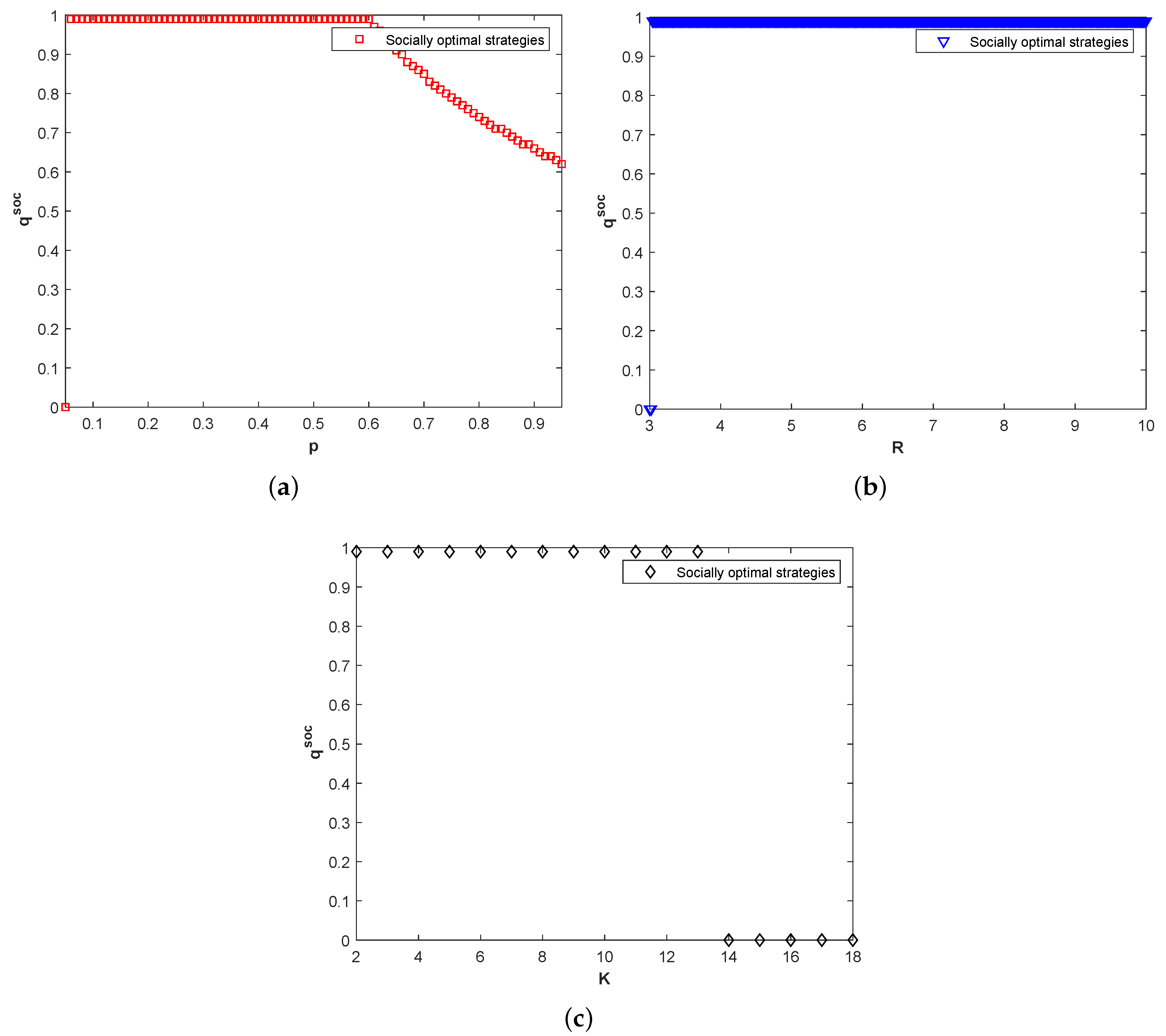
Figure 6 depict the socially optimal strategies in the fully unobservable case with respect to p, R and K. There is only one socially optimal strategy. Besides, 1 is always a socially optimal strategy in Figure 6b. The socially optimal strategy decreases with the increase of p and K, such as in Figure 6a,c.

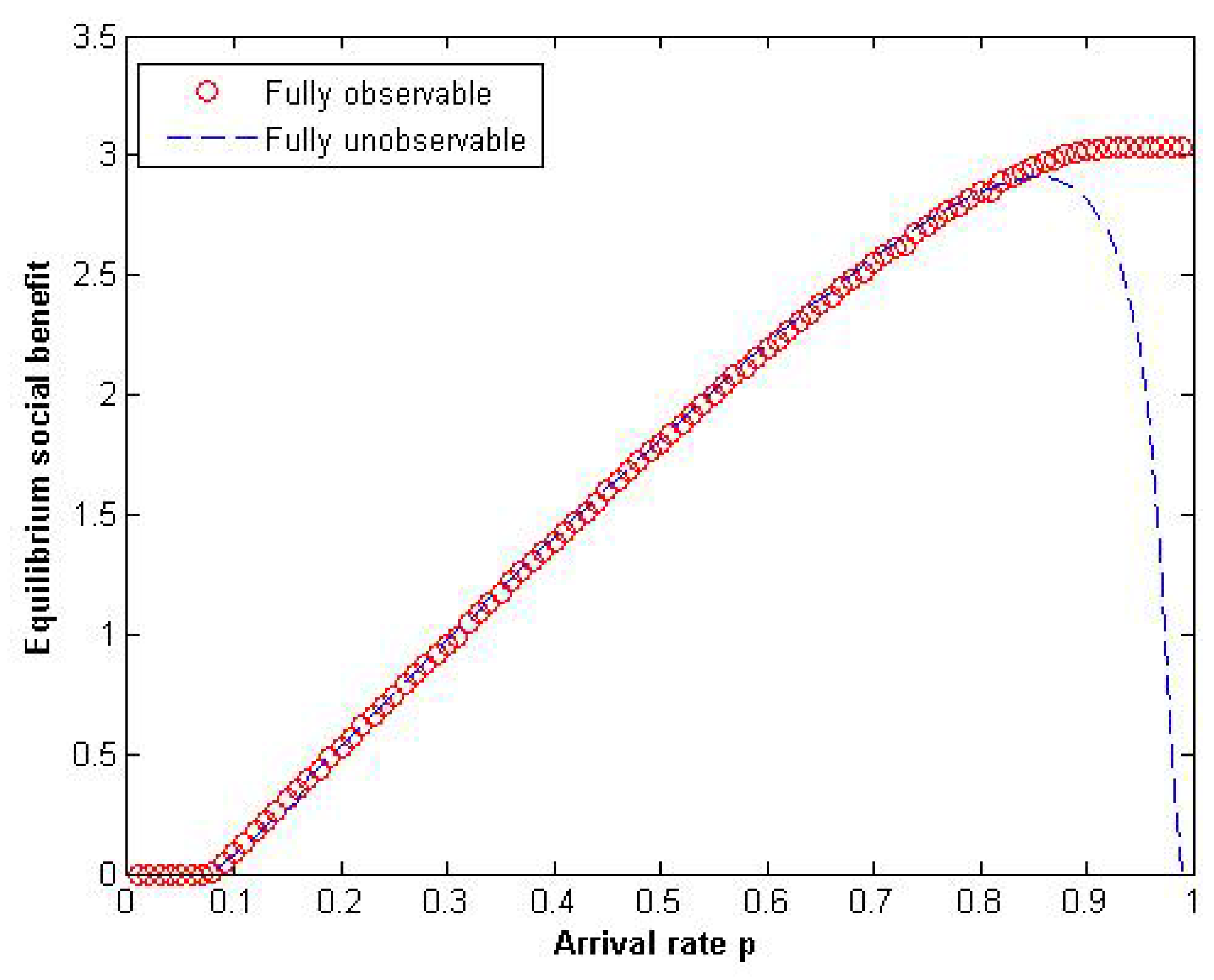
Second, we consider the relationship between the equilibrium social benefit and the variations in arrival rate p at two information levels. For $\mu =0.15,K=8,R=5$ and $C=0.1$, we explore the sensitivity of the equilibrium social benefit per time unit $B^{(o)}(m_0^{*})$ and $B^{(u)}(q)$ when arrival rate p varies in $(0,1)$, which is expected from Figure 7. Compared with continuous time batch service queueing systems, the discrete time batch service queueing systems have the following characteristics:

• While the value of p in the discrete time batch services ranges from 0 to 1, $\lambda$ can be any real number that is greater than 0 under the stationary condition.
• When p is less enough, under fully observable case and fully unobservable case, equilibrium social benefit is 0.
• For the most of p, the two kinds of information cases have similar values for the equilibrium social benefit.
• The equilibrium social benefit increases with respect to p in the fully observable case.
• For the high value of p, the fully observable case corresponds to the highest equilibrium social benefit, while congestion occurs in the fully unobservable case.

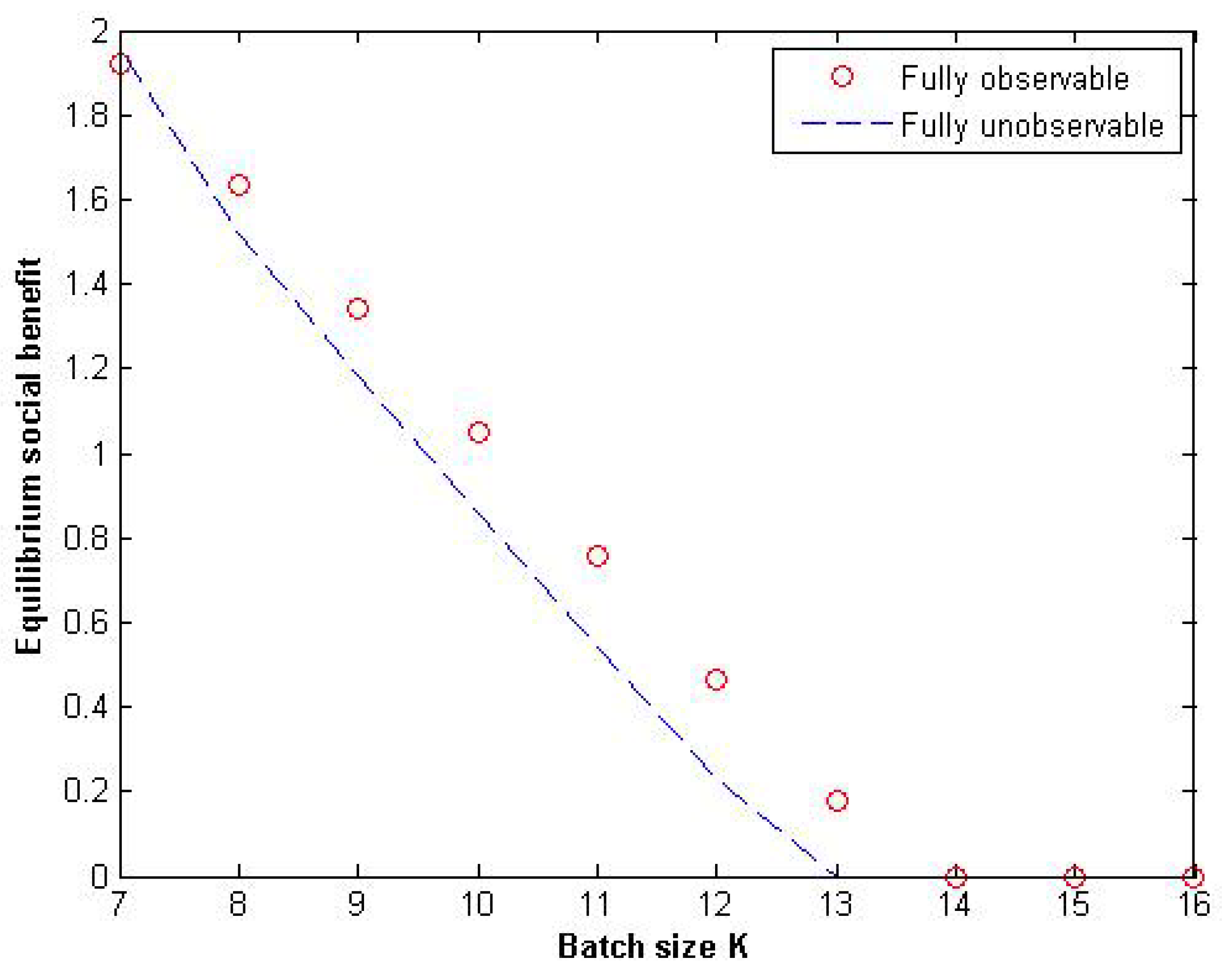
Finally, we research the equilibrium social benefit per time unit in model with the same parameters $p,R$ and C, that vary in $\mu$ and K but the overall service capacity $\mu K$ remains the same. Specifically, we study a model with $p=0.5,R=7,C=0.5$ and the overall service capacity $\mu K=6$. The batch size K changes in $\{7,8,\cdots ,16\}$, at the same time, $\mu$ varies in $\{\frac{6}{7},\frac{6}{8},\cdots ,\frac{6}{16}\}$. As a function of K, the equilibrium social benefit per time unit as a function of K is illustrated in Figure 8. We now can observe the following facts.

• In the fully unobservable case, the equilibrium social benefit decreases with the increase of K. However, the equilibrium social benefit is not a monotonic function of K in the fully observable case.
• In the fully observable case and the fully unobservable case, the functions of equilibrium social benefit do not intersect, although it may be the same for certain intervals of K.

We have a similar conclusion from the discrete time batch services and the continuous time bulk services. As can be seen from the experiments we have done, the graph of the fully unobservable case lies below the graph for the fully observable case. This fact is in agreement with the findings of the Markovian queue with batch services.

6. Conclusions and Future Research

In this paper, we have studied strategic behavior in the $Geo/Ge{o}^K/1$ queueing system under the fully observable case and the fully unobservable case. Besides, we extend the $M/M^K/1$ queueing system which was studied by Bountali and Economou [24] into the discrete-time batch service.

First, we compare the results obtained in this paper with those in continue time queueing systems. In the first place, we consider the relation between the strategic behavior in the $Geo/Ge{o}^K/1$ queueing system and corresponding in the $M/M^K/1$ queueing system. It is well known that if we assume that time is slotted into intervals of equal length $\Delta$, the $M/M^K/1$ queueing system can be approximated by the $Geo/Ge{o}^K/1$ where $\Delta$ is sufficiently small. Therefore, the outcome of Bountali and Economou [24] can be approximated by this paper. From the strategy of the customer, the results of these two models are consistent. Next, the conclusion is obviously different compared with $M/M/1$ queueing system. In the Edelson and Hildebrand [2]’s model, the equilibrium strategy is unique, while the equilibrium strategy in this paper is not. See Theorem 4 and Figure 5 for details. In the same way, in the observable case, the equilibrium strategy of Naor [1] is a single threshold strategy. The equilibrium strategy in this paper is double threshold strategy $(m_{K-1}^e,q_{m,j}^e)$, which is more complicated.

Second, we compared the result of Ma et al. [15] with this paper. In the Yan Ma et al.’s rest, the entrance probability is increasing with respect to R. However, the equilibrium strategy is decreasing with respect to R. At the same time, Ma’s individual equilibrium strategy is unique and this paper’s equilibrium strategies are one to three.

The further work of this paper is to study the strategic behavior of the customer in batch arrival or bulk service queueing system. For example the equilibrium strategy of the batch service in the almost observable case and almost unobservable case and so on. General service time and random batch service can be considered in the future. One can also consider the admission control problem in the $Geo/Ge{o}^K/1$ queueing systems.