Different Estimation Methods for Type I Half-Logistic Topp–Leone Distribution


Abstract
:1. Introduction
2. The Type I Half-Logistic Topp–Leone Distribution
3. Mathematical Properties
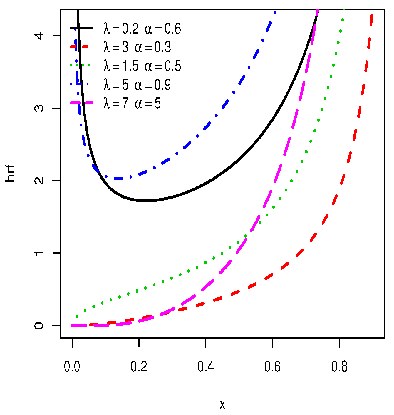
3.1. Asymptotes and Shapes
3.2. Quantile Function
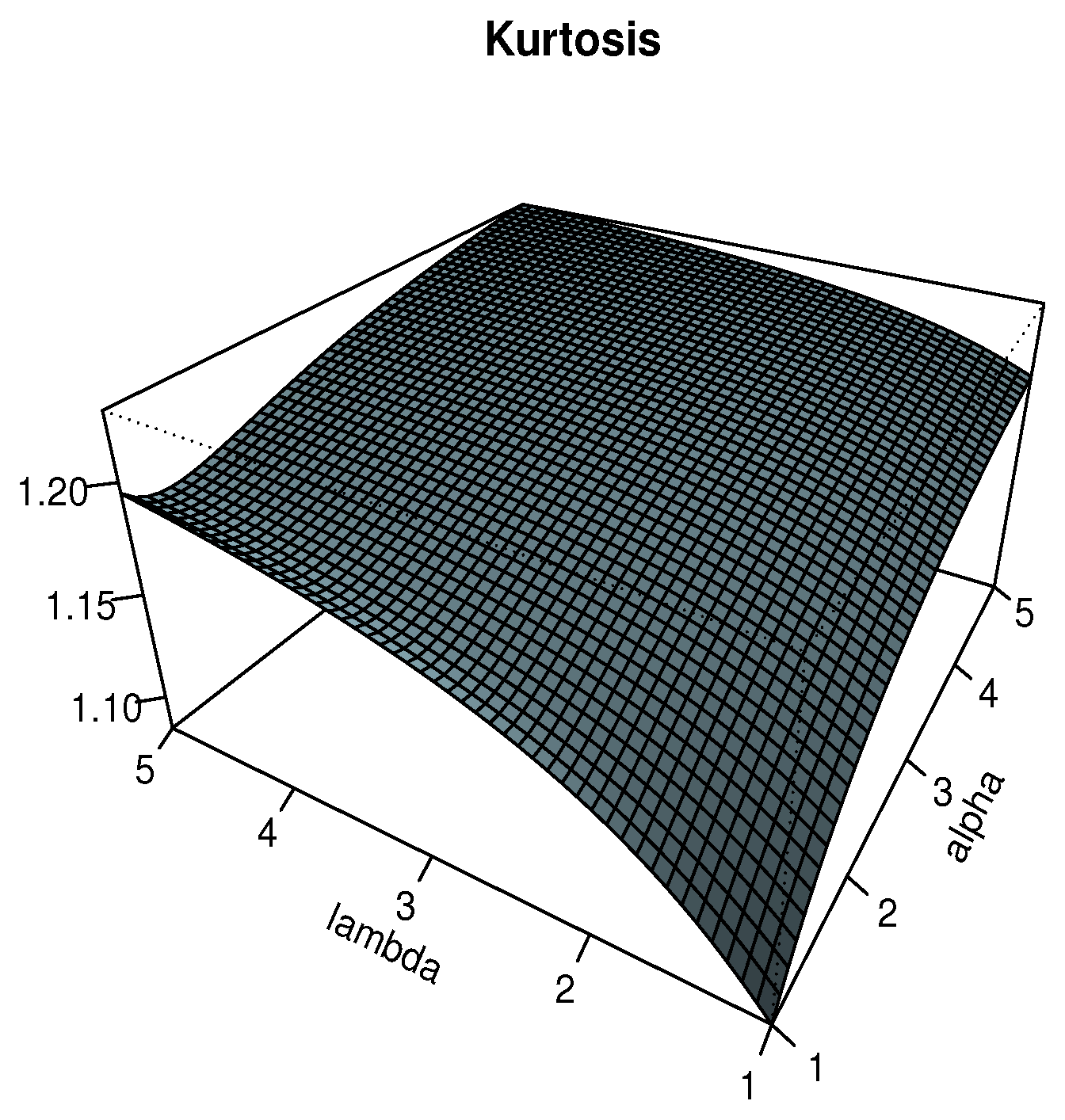
3.3. Skewness and Kurtosis
3.4. Power Series Expansion
3.5. Ordinary Moments
3.6. Incomplete Moments
3.7. Moment-Generating Function
3.8. Stress Strength Parameter
3.9. Order Statistics
4. Parameter Estimation
4.1. Method of Maximum Likelihood Estimation
4.2. Methods of Least Squares and Weighted Least Squares Estimation
4.3. Method of Cramer–von Mises Minimum Distance Estimation
4.4. Method of Percentile Estimation
4.5. Methods of Anderson–Darling and Right-Tail Anderson–Darling Estimation
4.6. Simulation
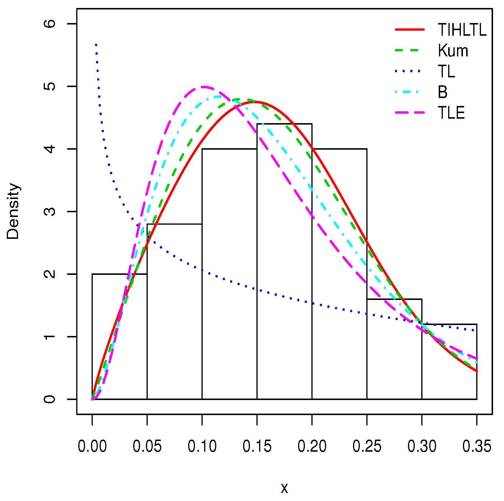
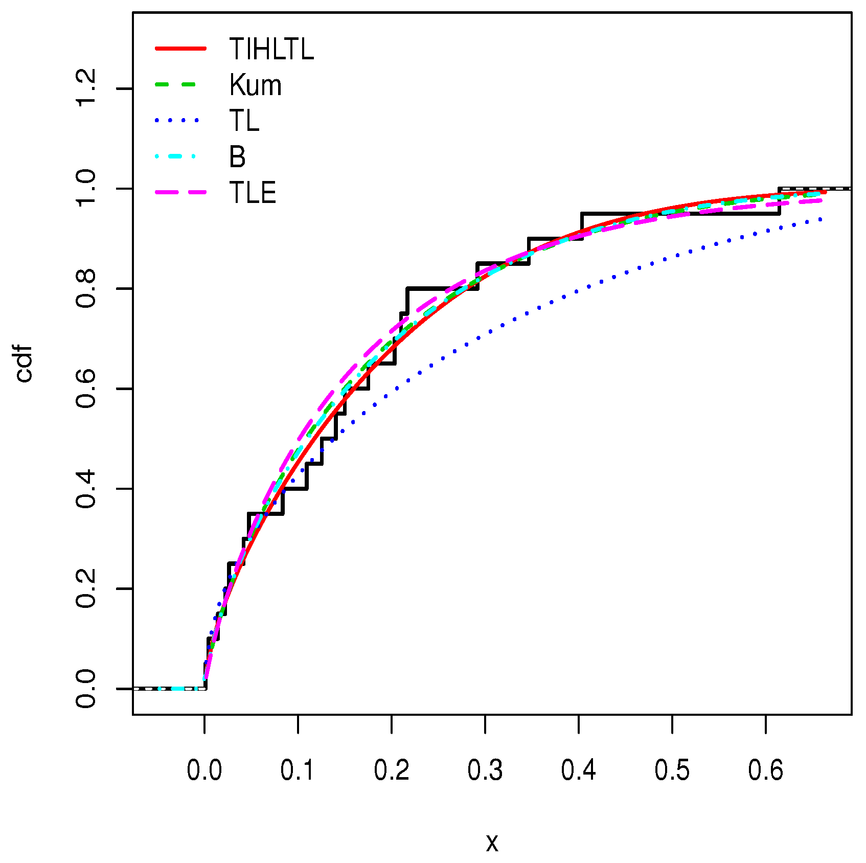
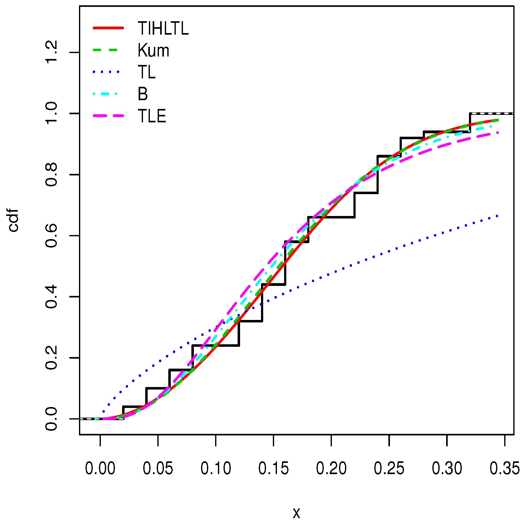
5. Applications
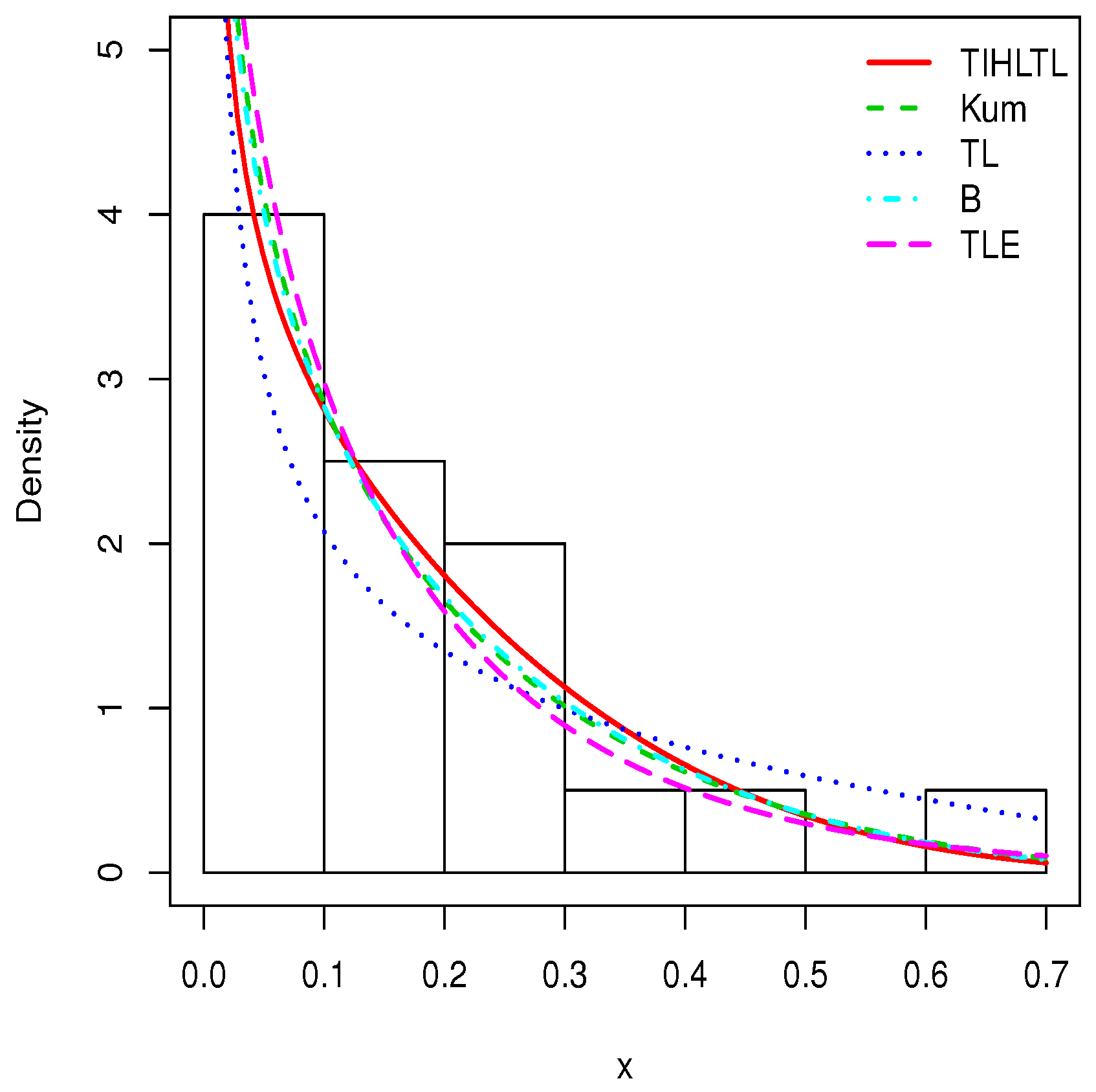
- The Kumaraswamy (Kum) model with pdf given bywhere ;
- The Topp–Leone (TL) model with pdf given bywhere ;
- The beta (B) model with pdf given bywhere and denotes the gamma function defined by ;
- The Topp–Leone exponential (TLE) model with pdf given bywhere . Further details on this distribution can be found in [29].
6. Concluding Remarks
Author Contributions
Funding
Acknowledgments
Conflicts of Interest
References
- Gupta, R.D.; Kundu, D. Exponentiated exponential family: An alternative to Gamma and Weibull distributions. Biom. J. 2001, 43, 117–130. [Google Scholar] [CrossRef]
- Eugene, N.; Lee, C.; Famoye, F. Beta-normal distribution and its applications. Commun. Stat.-Theory Methods 2002, 31, 497–512. [Google Scholar] [CrossRef]
- Zografos, K.; Balakrishnan, N. On families of beta- and generalized gamma-generated distributions and associated inference. Stat. Methodol. 2009, 6, 344–362. [Google Scholar] [CrossRef]
- Alizadeh, M.; Emadiz, M.; Doostparast, M.; Cordeiro, G.M.; Ortega, E.M.M.; Pescim, R.R. A new family of distributions: The Kumaraswamy odd log-logistic, properties and applications. Hacet. J. Math. Stat. 2015, 44, 1491–1512. [Google Scholar] [CrossRef]
- Cordeiro, G.M.; Alizadeh, M.; Marinho, E.P.R.D. The type I half-logistic family of distributions. J. Stat. Comput. Simul. 2015, 86, 707–728. [Google Scholar] [CrossRef]
- Cordeiro, G.M.; Alizadeh, M.; Ozel, G. The generalized odd log-logistic family of distributions: Properties, regression models and applications. J. Stat. Comput. Simul. 2017, 87, 908–932. [Google Scholar] [CrossRef]
- Alizadeh, M.; Altun, E.; Cordeiro, G.M.; Rasekhi, M. The odd power Cauchy family of distributions: Properties, regression models and applications. J. Stat. Comput. Simul. 2018, 88, 785–805. [Google Scholar] [CrossRef]
- Reyad, H.M.; Alizadeh, M.; Jamal, F.; Othman, S.; Hamedani, G.G. The Exponentiated Generalized Topp Leone-G Family of Distributions: Properties and Applications. Pak. J. Stat. Oper. Res. 2019, 15, 1–24. [Google Scholar] [CrossRef]
- Jamal, F.; Chesneau, C.; Elgarhy, M. Type II general inverse exponential family of distributions. J. Stat. Manag. Syst. 2019. Available online: https://www.tandfonline.com/toc/tsms20/current (accessed on 15 August 2019).
- Topp, C.W.; Leone, F.C. A family of J-shaped frequency functions. J. Am. Stat. Assoc. 1955, 50, 209–219. [Google Scholar] [CrossRef]
- Nadarajah, S.; Kotz, S. Moments of some J-shaped distributions. J. Appl. Stat. 2003, 30, 311–317. [Google Scholar] [CrossRef]
- Ghitany, M.E.; Kotz, S.; Xie, M. On some reliability measures and their stochastic orderings for the Topp-Leone distribution. J. Appl. Stat. 2005, 32, 715–722. [Google Scholar] [CrossRef]
- Sangsanit, Y.; Bodhisuwan, W. The Topp-Leone generator of distributions: Properties and inferences. Songklanakarin J. Sci. Technol. 2016, 38, 537–548. [Google Scholar]
- Kunjiratanachot, N.; Bodhisuwan, W.; Volodin, A. The Topp-Leone generalized exponential power series distribution with applications. J. Probab. Stat. Sci. 2018, 16, 197–208. [Google Scholar]
- Elgarhy, M.; Nasir, M.A.; Jamal, F.; Ozel, G. The type II Topp-Leone generated family of distributions: Properties and applications. J. Stat. Manag. Syst. 2018, 21, 1529–1551. [Google Scholar] [CrossRef]
- Mauldon, J.M. A Generalization of the Beta-distribution. Ann. Math. Stat. 1959, 30, 509–520. [Google Scholar] [CrossRef]
- Kumaraswamy, P. A generalized probability density function for double-bounded random processes. J. Hydrol. 1980, 46, 79–88. [Google Scholar] [CrossRef]
- Abramowitz, M.; Stegun, I.A. Handbook of Mathematical Functions, National Bureau of Standards; Applied Math. Series 55; Dover Publications: Mineola, NY, USA, 1965. [Google Scholar]
- Galton, F. Inquiries Into Human Faculty and Its Development; Macmillan and Company: London, UK, 1883. [Google Scholar]
- Moors, J.J.A. A quantile alternative for Kurtosis. J. R. Stat. Soc. Ser. D (Stat.) 1988, 37, 25–32. [Google Scholar] [CrossRef]
- Kotz, S.; Lumelskii, Y.; Penskey, M. The Stress-Strength Model and Its Generalizations and Applications; World Scientific: Singapore, 2003. [Google Scholar]
- David, H.A.; Nagaraja, H.N. Order Statistics; John Wiley and Sons: Hoboken, NJ, USA, 2003. [Google Scholar]
- Casella, G.; Berger, R.L. Statistical Inference; Brooks/Cole Publishing Company: Bel Air, CA, USA, 1990. [Google Scholar]
- Swain, J.J.; Venkatraman, S.; Wilson, J.R. Least-squares estimation of distribution functions in johnson’s translation system. J. Stat. Comput. Simul. 1988, 29, 271–297. [Google Scholar] [CrossRef]
- Macdonald, P.D.M. Comment on ‘An estimation procedure for mixtures of distributions’ by Choi and Bulgren. J. R. Stat. Soc. B 1971, 33, 326–329. [Google Scholar]
- Kao, J. Computer methods for estimating Weibull parameters in reliability studies. IRE Trans. Reliab. Qual. Control 1958, 13, 15–22. [Google Scholar] [CrossRef]
- Kao, J. A graphical estimation of mixed Weibull parameters in life testing electron tube. Technometrics 1959, 1, 389–407. [Google Scholar] [CrossRef]
- Anderson, T.W.; Darling, D.A. Asymptotic theory of certain ‘goodness-of- fit’ criteria based on stochastic processes. Ann. Math. Stat. 1952, 23, 193–212. [Google Scholar] [CrossRef]
- Al-Shomrani, A.; Arif, O.; Shawky, K.; Hanif, S.; Shahbaz, M.Q. Topp-Leone family of distributions: Some properties and application. Pak. J. Stat. Oper. Res. 2016, 12, 443–451. [Google Scholar] [CrossRef]
- Nigm, A.M.; AL-Hussaini, E.K.; Jaheen, Z.F. Bayesian one sample prediction of future observations under Pareto distribution. Statistics 2003, 37, 527–536. [Google Scholar] [CrossRef]
- Dasgupta, R. On the distribution of Burr with applications. Sankhya 2011, 73, 1–19. [Google Scholar] [CrossRef]
- Aarset, M.V. How to identify bathtub hazard rate. IEEE Trans. Reliab. 1987, 36, 106–108. [Google Scholar] [CrossRef]


| MLE | LSE | WLSE | PCE | CVE | ADE | RTADE | ||||||||
|---|---|---|---|---|---|---|---|---|---|---|---|---|---|---|
| n | Est. | MSEs | Est. | MSEs | Est. | MSEs | Est. | MSEs | Est. | MSEs | Est. | MSEs | Est. | MSEs |
| 50 | 2.172 | 0.628 | 2.038 | 0.473 | 2.058 | 0.508 | 1.808 | 0.583 | 2.148 | 3.377 | 2.067 | 2.974 | 2.194 | 3.811 |
| 0.507 | 7.116 * | 0.499 | 5.885 * | 0.498 | 6.713 * | 0.472 | 0.013 | 0.499 | 6.241 * | 0.499 | 6.682 * | 0.498 | 7.554 * | |
| 100 | 2.164 | 0.271 | 2.011 | 0.206 | 2.062 | 0.340 | 1.852 | 0.272 | 2.159 | 3.139 | 2.064 | 2.766 | 2.131 | 3.288 |
| 0.515 | 2.525 * | 0.499 | 2.756 * | 0.495 | 2.766 * | 0.473 | 7.531 * | 0.515 | 3.873 * | 0.496 | 2.697 * | 0.501 | 3.809 * | |
| 200 | 2.106 | 0.098 | 2.023 | 0.157 | 2.029 | 0.107 | 1.912 | 0.130 | 2.057 | 2.587 | 2.015 | 2.379 | 2.030 | 2.532 |
| 0.503 | 1.184 * | 0.500 | 1.891 * | 0.502 | 1.514 * | 0.488 | 4.459 * | 0.501 | 1.827 * | 0.501 | 1.220 * | 0.501 | 1.848 * | |
| 1000 | 1.997 | 0.057 | 2.012 | 0.024 | 2.012 | 0.019 | 1.998 | 0.039 | 2.020 | 2.334 | 2.010 | 2.298 | 2.027 | 2.365 |
| 0.499 | 1.381 * | 0.501 | 0.313 * | 0.501 | 0.247 * | 0.503 | 1.741 * | 0.502 | 0.317 * | 0.501 | 0.251 * | 0.502 | 0.324 * |
| MLE | LSE | WLSE | PCE | CVE | ADE | RTADE | ||||||||
|---|---|---|---|---|---|---|---|---|---|---|---|---|---|---|
| n | Est. | MSEs | Est. | MSEs | Est. | MSEs | Est. | MSEs | Est. | MSEs | Est. | MSEs | Est. | MSEs |
| 50 | 2.136 | 0.213 | 1.949 | 0.188 | 2.049 | 0.210 | 1.794 | 0.272 | 2.092 | 0.614 | 2.043 | 0.456 | 2.130 | 0.679 |
| 1.593 | 0.106 | 1.465 | 0.064 | 1.538 | 0.114 | 1.350 | 0.153 | 1.588 | 0.135 | 1.552 | 0.081 | 1.573 | 0.136 | |
| 100 | 2.063 | 0.077 | 2.051 | 0.130 | 2.008 | 0.118 | 1.780 | 0.181 | 2.079 | 0.438 | 2.012 | 0.346 | 2.069 | 0.470 |
| 1.535 | 0.033 | 1.539 | 0.051 | 1.502 | 0.046 | 1.333 | 0.167 | 1.565 | 0.050 | 1.504 | 0.030 | 1.535 | 0.050 | |
| 200 | 2.026 | 0.047 | 2.016 | 0.057 | 2.021 | 0.047 | 1.850 | 0.085 | 2.055 | 0.370 | 2.011 | 0.312 | 2.042 | 0.340 |
| 1.529 | 0.018 | 1.516 | 0.026 | 1.528 | 0.022 | 1.387 | 0.069 | 1.543 | 0.030 | 1.503 | 0.022 | 1.540 | 0.021 | |
| 1000 | 2.009 | 7.847 * | 2.007 | 0.010 | 2.008 | 8.377 * | 1.961 | 0.016 | 2.012 | 0.272 | 2.006 | 0.265 | 2.014 | 0.276 |
| 1.507 | 3.286 * | 1.505 | 4.59 *1 | 1.506 | 3.595 * | 1.465 | 0.013 | 1.509 | 4.675 * | 1.505 | 3.699 * | 1.510 | 4.574 * |
| MLE | LSE | WLSE | PCE | CVE | ADE | RTADE | ||||||||
|---|---|---|---|---|---|---|---|---|---|---|---|---|---|---|
| n | Est. | MSEs | Est. | MSEs | Est. | MSEs | Est. | MSEs | Est. | MSEs | Est. | MSEs | Est. | MSEs |
| 50 | 2.065 | 0.164 | 2.034 | 0.199 | 2.060 | 0.204 | 1.781 | 0.274 | 2.104 | 0.238 | 2.012 | 0.157 | 2.078 | 0.230 |
| 2.089 | 0.161 | 2.047 | 0.230 | 2.071 | 0.226 | 1.790 | 0.474 | 2.144 | 0.332 | 2.042 | 0.153 | 2.105 | 0.255 | |
| 100 | 2.028 | 0.071 | 1.984 | 0.083 | 2.035 | 0.105 | 1.861 | 0.139 | 2.058 | 0.092 | 2.032 | 0.071 | 2.047 | 0.101 |
| 2.033 | 0.088 | 2.002 | 0.084 | 2.068 | 0.122 | 1.856 | 0.212 | 2.094 | 0.122 | 2.051 | 0.075 | 2.074 | 0.102 | |
| 200 | 2.023 | 0.043 | 2.014 | 0.051 | 2.014 | 0.034 | 1.932 | 0.060 | 2.016 | 0.052 | 2.026 | 0.038 | 1.995 | 0.049 |
| 2.038 | 0.043 | 2.005 | 0.063 | 2.017 | 0.031 | 1.920 | 0.117 | 2.013 | 0.067 | 2.037 | 0.038 | 1.993 | 0.039 | |
| 1000 | 2.008 | 6.831 * | 2.007 | 8.687 * | 2.008 | 7.203 * | 1.966 | 0.014 | 2.011 | 8.796 * | 2.006 | 7.359 * | 2.012 | 0.010 |
| 2.010 | 6.858 * | 2.008 | 9.561 * | 2.010 | 7.461 * | 1.955 | 0.028 | 2.013 | 9.735 * | 2.008 | 7.691 * | 2.014 | 9.411 * |
| MLE | LSE | WLSE | PCE | CVE | ADE | RTADE | ||||||||
|---|---|---|---|---|---|---|---|---|---|---|---|---|---|---|
| n | Est. | MSEs | Est. | MSEs | Est. | MSEs | Est. | MSEs | Est. | MSEs | Est. | MSEs | Est. | MSEs |
| 50 | 3.392 | 1.117 | 3.173 | 1.883 | 3.285 | 1.993 | 2.624 | 1.241 | 3.460 | 10.441 | 3.183 | 8.504 | 3.435 | 11.453 |
| 0.521 | 6.864 * | 0.505 | 7.689 * | 0.514 | 9.365 * | 0.470 | 0.016 | 0.523 | 8.203 * | 0.507 | 6.952 * | 0.513 | 7.557 * | |
| 100 | 3.163 | 0.486 | 3.186 | 0.794 | 3.043 | 0.579 | 2.720 | 0.735 | 3.373 | 9.084 | 3.102 | 7.179 | 3.163 | 7.792 |
| 0.507 | 2.750 * | 0.506 | 4.799 * | 0.502 | 2.578 * | 0.470 | 8.690 * | 0.518 | 5.421 * | 0.508 | 2.955 * | 0.505 | 2.814 * | |
| 200 | 3.047 | 0.204 | 3.121 | 0.485 | 3.059 | 0.208 | 2.890 | 0.357 | 3.133 | 7.383 | 3.027 | 6.630 | 3.159 | 7.470 |
| 0.506 | 1.541 * | 0.505 | 1.617 * | 0.503 | 0.950 * | 0.478 | 5.915 * | 0.506 | 1.689 * | 0.499 | 1.462 * | 0.503 | 1.766 * | |
| 1000 | 3.026 | 0.040 | 3.018 | 0.054 | 3.018 | 0.042 | 2.950 | 0.064 | 3.030 | 6.453 | 3.015 | 6.366 | 3.041 | 6.529 |
| 0.502 | 0.227 * | 0.501 | 0.313 * | 0.501 | 0.246 * | 0.496 | 0.976 * | 0.502 | 0.317 * | 0.501 | 0.251 * | 0.502 | 0.324 * |
| MLE | LSE | WLSE | PCE | CVE | ADE | RTADE | ||||||||
|---|---|---|---|---|---|---|---|---|---|---|---|---|---|---|
| n | Est. | MSEs | Est. | MSEs | Est. | MSEs | Est. | MSEs | Est. | MSEs | Est. | MSEs | Est. | MSEs |
| 50 | 3.008 | 0.367 | 3.058 | 0.490 | 3.070 | 0.463 | 2.771 | 0.654 | 3.224 | 3.577 | 3.105 | 2.921 | 3.049 | 2.902 |
| 1.567 | 0.090 | 1.551 | 0.110 | 1.495 | 0.069 | 1.451 | 0.282 | 1.639 | 0.149 | 1.538 | 0.068 | 1.518 | 0.078 | |
| 100 | 3.190 | 0.256 | 3.103 | 0.350 | 3.111 | 0.206 | 2.753 | 0.323 | 3.191 | 3.182 | 3.016 | 2.522 | 3.020 | 2.630 |
| 1.582 | 0.059 | 1.554 | 0.076 | 1.536 | 0.041 | 1.374 | 0.127 | 1.601 | 0.089 | 1.506 | 0.036 | 1.518 | 0.058 | |
| 200 | 3.050 | 0.081 | 2.946 | 0.157 | 3.073 | 0.144 | 2.777 | 0.199 | 3.001 | 2.408 | 3.002 | 2.379 | 3.034 | 2.476 |
| 1.530 | 0.018 | 1.485 | 0.030 | 1.523 | 0.027 | 1.378 | 0.069 | 1.510 | 0.033 | 1.498 | 0.023 | 1.521 | 0.023 | |
| 1000 | 3.014 | 0.018 | 3.011 | 0.023 | 3.014 | 0.019 | 2.942 | 0.036 | 3.018 | 2.329 | 3.010 | 2.298 | 3.021 | 2.340 |
| 1.507 | 3.265 * | 1.505 | 4.599 * | 1.507 | 3.676 * | 1.465 | 0.013 | 1.509 | 4.686 * | 1.505 | 3.698 * | 1.510 | 4.575 * |
| MLE | LSE | WLSE | PCE | CVE | ADE | RTADE | ||||||||
|---|---|---|---|---|---|---|---|---|---|---|---|---|---|---|
| n | Est. | MSEs | Est. | MSEs | Est. | MSEs | Est. | MSEs | Est. | MSEs | Est. | MSEs | Est. | MSEs |
| 50 | 3.165 | 0.341 | 2.996 | 0.360 | 3.003 | 0.335 | 2.723 | 0.747 | 3.125 | 1.686 | 3.040 | 1.500 | 3.109 | 1.676 |
| 2.101 | 0.204 | 2.001 | 0.183 | 2.049 | 0.154 | 1.861 | 0.448 | 2.125 | 0.227 | 2.093 | 0.200 | 2.081 | 0.212 | |
| 100 | 3.085 | 0.177 | 3.022 | 0.226 | 3.113 | 0.209 | 2.692 | 0.317 | 3.048 | 1.318 | 3.029 | 1.253 | 3.059 | 1.324 |
| 2.048 | 0.076 | 2.045 | 0.173 | 2.099 | 0.110 | 1.765 | 0.239 | 2.054 | 0.147 | 2.030 | 0.088 | 2.037 | 0.086 | |
| 200 | 2.993 | 0.073 | 3.032 | 0.100 | 2.988 | 0.101 | 2.825 | 0.193 | 3.102 | 1.321 | 3.025 | 1.118 | 3.004 | 1.145 |
| 1.998 | 0.036 | 2.031 | 0.045 | 1.997 | 0.048 | 1.866 | 0.128 | 2.078 | 0.060 | 2.015 | 0.034 | 2.030 | 0.062 | |
| 1000 | 3.012 | 0.015 | 3.010 | 0.020 | 3.010 | 0.016 | 2.942 | 0.034 | 3.017 | 1.054 | 3.009 | 1.034 | 3.018 | 1.060 |
| 2.010 | 6.858 * | 2.008 | 9.564 * | 2.009 | 7.425 * | 1.947 | 0.029 | 2.013 | 9.728 * | 2.008 | 7.689 * | 2.014 | 9.413 * |
| Parameters | n | MLE | LSE | WLSE | PCE | CVE | ADE | RTADE |
|---|---|---|---|---|---|---|---|---|
| , | 50 | 4.5 | 1.0 | 2.0 | 6.0 | 3.0 | 4.5 | 7.0 |
| 100 | 1.0 | 2.0 | 3.5 | 5.0 | 6.5 | 4.5 | 6.5 | |
| 200 | 1.0 | 4.5 | 2.0 | 4.5 | 6.5 | 3.0 | 6.5 | |
| 1000 | 5.5 | 2.0 | 1.0 | 5.5 | 3.5 | 3.5 | 7.0 | |
| , | 50 | 2.5 | 1.0 | 2.5 | 5.0 | 6.5 | 4.0 | 6.5 |
| 100 | 1.0 | 4.0 | 2.0 | 6.0 | 5.0 | 3.0 | 7.0 | |
| 200 | 1.0 | 3.0 | 2.0 | 6.0 | 7.0 | 5.0 | 4.0 | |
| 1000 | 1.0 | 3.5 | 2.0 | 5.5 | 7.0 | 3.5 | 5.5 | |
| , | 50 | 2.0 | 3.5 | 3.5 | 7.0 | 6.0 | 1.0 | 5.0 |
| 100 | 2.0 | 3.0 | 6.0 | 7.0 | 5.0 | 1.0 | 4.0 | |
| 200 | 3.5 | 5.0 | 1.0 | 7.0 | 6.0 | 2.0 | 3.5 | |
| 1000 | 1.0 | 4.0 | 2.0 | 7.0 | 5.0 | 7.0 | 6.0 | |
| , | 50 | 1.0 | 2.5 | 5.5 | 4.0 | 7.0 | 2.5 | 5.5 |
| 100 | 1.5 | 3.0 | 1.5 | 6.0 | 7.0 | 3.0 | 3.0 | |
| 200 | 2.0 | 4.0 | 1.0 | 5.0 | 6.0 | 3.0 | 7.0 | |
| 1000 | 1.0 | 3.0 | 2.0 | 5.5 | 5.5 | 4.0 | 7.0 | |
| , | 50 | 1.5 | 4.5 | 1.5 | 6.0 | 7.0 | 3.0 | 4.5 |
| 100 | 2.5 | 4.5 | 1.0 | 6.0 | 7.0 | 2.5 | 4.5 | |
| 200 | 1.0 | 4.0 | 2.0 | 6.0 | 7.0 | 3.0 | 5.0 | |
| 1000 | 1.0 | 3.5 | 2.0 | 5.5 | 7.0 | 3.5 | 5.5 | |
| , | 50 | 2.5 | 1.0 | 2.5 | 7.0 | 6.0 | 4.0 | 5.0 |
| 100 | 1.5 | 5.5 | 3.0 | 7.5 | 1.5 | 7.5 | 4.0 | |
| 200 | 1.0 | 2.5 | 4.0 | 5.5 | 5.5 | 2.5 | 7.0 | |
| 1000 | 1.0 | 3.5 | 2.0 | 5.5 | 7.0 | 3.5 | 5.5 | |
| Sum of ranks | 43.5 | 78 | 57.5 | 141 | 140.5 | 84 | 132 | |
| Overall rank | 1 | 3 | 2 | 7 | 6 | 4 | 5 |
| n | Mean | Median | Standard Deviation | Skewness | Kurtosis | |
|---|---|---|---|---|---|---|
| Data set 1 | 20 | 0.16 | 0.13 | 0.16 | 1.23 | 1.07 |
| Data set 2 | 50 | 0.16 | 0.16 | 0.08 | 0.07 | −0.87 |
| Model | λ | α | a | b |
|---|---|---|---|---|
| TIHLTL | 2.1342 | 0.6028 | - | - |
| (0.6336) | (0.1706) | - | - | |
| Kum | - | - | 0.7639 | 3.4341 |
| - | - | (0.1751) | (1.3113) | |
| TL | - | 0.5112 | - | - |
| - | (0.1143) | - | - | |
| B | - | - | 0.7134 | 3.7459 |
| - | - | (0.1931) | ( 1.3085) | |
| TLE | 0.7925 | 2.6644 | - | - |
| (0.2208) | (0.8240) | - | - |
| Model | λ | α | a | b |
|---|---|---|---|---|
| TIHLTL | 10.6094 | 1.8752 | - | - |
| (1.1160) | (0.2643) | - | - | |
| Kum | - | - | 2.0750 | 33.0041 |
| - | - | (0.2542) | (3.8351) | |
| TL | - | 0.7247 | - | - |
| - | (0.1024) | - | - | |
| B | - | - | 2.6799 | 13.8502 |
| - | - | (0.5066) | (2.8249) | |
| TLE | 3.1718 | 5.6800 | - | - |
| (0.7067) | (0.7841) | - | - |
| Model | AIC | BIC | W* | A* | KS | p-Value (KS) | |
|---|---|---|---|---|---|---|---|
| TIHLTL | −17.3028 | −30.6057 | −28.6143 | 0.0208 | 0.1348 | 0.0900 | 0.9912 |
| Kum | −17.2047 | −30.4094 | −28.4180 | 0.0289 | 0.1691 | 0.1026 | 0.9700 |
| TL | −15.6166 | −29.2333 | −28.2376 | 0.0300 | 0.1754 | 0.1848 | 0.4481 |
| B | −17.2532 | −30.5064 | −28.5150 | 0.0263 | 0.1565 | 0.0980 | 0.9782 |
| TLE | −16.8608 | −29.7216 | −27.7301 | 0.0375 | 0.2124 | 0.1225 | 0.8899 |
| Model | AIC | BIC | W* | A* | KS | p-Value (KS) | |
|---|---|---|---|---|---|---|---|
| TIHLTL | −56.4261 | −108.8522 | −105.0282 | 0.0893 | 0.5496 | 0.1031 | 0.6623 |
| Kum | −56.0686 | −108.1373 | −104.3132 | 0.1024 | 0.6248 | 0.1104 | 0.5755 |
| TL | −28.4078 | −54.8156 | −52.9035 | 0.1653 | 0.9919 | 0.3622 | 0.000003 |
| B | −54.6066 | −105.2133 | −101.3892 | 0.1479 | 0.8926 | 0.1414 | 0.2697 |
| TLE | −52.2862 | −100.5725 | −96.7484 | 0.2120 | 1.2634 | 0.1652 | 0.1302 |
| CI | λ | α |
| 95% | [0.8923 3.3760] | [0.2684 0.9371] |
| 99% | [0.4995 3.7688] | [0.1626 1.0429] |
| CI | λ | α |
| 95% | [8.4220 12.7967] | [1.3571 2.3932] |
| 99% | [7.7301 13.4886] | [1.1933 2.5570] |
© 2019 by the authors. Licensee MDPI, Basel, Switzerland. This article is an open access article distributed under the terms and conditions of the Creative Commons Attribution (CC BY) license (http://creativecommons.org/licenses/by/4.0/).
Share and Cite
ZeinEldin, R.A.; Chesneau, C.; Jamal, F.; Elgarhy, M. Different Estimation Methods for Type I Half-Logistic Topp–Leone Distribution. Mathematics 2019, 7, 985. https://doi.org/10.3390/math7100985
ZeinEldin RA, Chesneau C, Jamal F, Elgarhy M. Different Estimation Methods for Type I Half-Logistic Topp–Leone Distribution. Mathematics. 2019; 7(10):985. https://doi.org/10.3390/math7100985
Chicago/Turabian StyleZeinEldin, Ramadan A., Christophe Chesneau, Farrukh Jamal, and Mohammed Elgarhy. 2019. "Different Estimation Methods for Type I Half-Logistic Topp–Leone Distribution" Mathematics 7, no. 10: 985. https://doi.org/10.3390/math7100985
APA StyleZeinEldin, R. A., Chesneau, C., Jamal, F., & Elgarhy, M. (2019). Different Estimation Methods for Type I Half-Logistic Topp–Leone Distribution. Mathematics, 7(10), 985. https://doi.org/10.3390/math7100985